Assessing transition probability of bridge deterioration using Dempster

Abstract

Reliable deterioration models for forecasting the condition of bridge elements, systems, and networks are essential components of any bridge management system. Estimating deterioration transition probabilities is the basis of the popular Markov chain deterioration model. Transition probabilities have been produced in the literature by statistical and probabilistic analysis performed on available bridge inspection and condition data. The available data may be limited or inconsistent with the Markov chain transition period. In addition, the conventional probability theory has limitations when applied to problems with a stochastic nature such as bridge deterioration. This paper introduces a novel method based on the theory of evidence for bridge deterioration modeling through expert judgment elicitation. The advantages of the theory of evidence over the traditional probability theory are discussed and the process for the theory implementation is demonstrated with a case study to validate the application of Dempster–Shafer theory of evidence to estimate the transition probabilities. Based on the results, the theory of evidence is proposed as a scientific expert judgement elicitation technique in the area of bridge condition rating and deterioration modeling. Expert judgment elicitation and theory of evidence application hold potential in the field of bridge management and require further investigation and research.

Keywords

Bridge deterioration transition probability markov chains Dempster–Shafer theory of evidence

1 Introduction

Transportation infrastructure is a major component of most civil infrastructure systems and can be considered as one of society’s critical foundations. Bridges in particular are especially important because of their distinct function of joining highways and roadways as crucial nodes. The deterioration of bridge infrastructure imposes major safety and economic concerns. Several countries have started to develop and use Bridge Management Systems (BMSs) to assist practitioners in making effective bridge management decisions. For instance, Pontis (currently known as BrM) is an advanced BMS that has been used by departments of transportation across the United States. The FHWA [8] reported that Pontis was used by 39 states, 5 municipalities, and 5 international agencies. Provincial ministries of transportation in Canada, including Ontario and Quebec, have started their own programs to develop and use BMSs [7, 26]. Among the BMSs in Europe are Danbro in Denmark and Finish in Finland. Other country-specific BMSs include those utilized in Australia, the Netherlands, Germany, France, UK, Norway, Spain, Finland, Poland, and Japan. The AASHTO guidelines for bridge management systems [3] specified that reliable deterioration models to predict the future condition of bridge elements, systems, and networks are indispensable components of any BMS.

State-of-the-art bridge management systems have adopted Markov chains model as a stochastic approach for predicting performance of bridge elements and bridge networks. Among the systems that have implemented Markov chains model: Pontis [10], BRIDGIT [13] and the Ontario Bridge Management System [26]. Estimating transition probabilities is the basis of Markov chains model. A transition probability is the chance of deterioration from one condition state to another during one discrete transition period. These probabilities are obtained either from accumulated inspection and condition data or by using expert judgment elicitation procedures through soliciting input of experienced bridge engineers [27, 21].

2 Research objective and methodology

The research aimed to study the available methods to estimate transition probabilities necessary for the implementation of the Markov chain deterioration model and to introduce a new approach to circumvent some of the limitation associated with these methods. The research methodology comprises the following stages:

Review the literature on the available methods to estimate transition probabilities of bridge deterioration process and to discuss these methods and their limitations.

Propose an alternative technique to estimate transition probabilities while accounting for the main limitations identified in the previous stage to better understand the deterioration process and to enhance predictions.

Demonstrate and validate the proposed technique with a case study.

The following sections explain the implementation of the research methodology. This methodology concluded with the development of a novel technique based on Dempster–Shafer (D–S) theory of evidence for estimating transition probabilities through expert judgment elicitation.

3 Transition probability

The popular Markov chains deterioration model characterizes probability of a facility to undergo a transition in condition state at a given discrete time interval. Estimated transition probabilities are assembled in a matrix of order of (n×n) known as the transition matrix, where n is the number of possible condition states. For example, element p_ij in the matrix is the transition probability from state i to state j during a discrete transition period. Condition prediction after any number of transition periods can be accomplished by multiplying the current or initial condition vector by the transition probability matrix [15]. If P(0) is the initial condition vector and describes the present condition of a bridge element, the future condition vector P(t) at any number of transition periods (t) from now can be predicted by multiplying the initial condition vector by the transition probability matrix as follows: $P (t) = P (0) \times P^{t}$ (1)

where $P = [\begin{matrix} p_{11} & \dots & p_{1 n} \\ \dots & \dots & \dots \\ p_{n 1} & \dots & p_{nn} \end{matrix}]$

Estimated transition probabilities discussed in the literature are developed by analyzing condition data extracted from bridge inspection databases and condition rating reports. Two methods are typically used to generate transition probability matrices from the available condition data. These methods are regression-based optimization and the percentage prediction method. The regression-based optimization estimates transition probabilities by minimizing the sum of absolute differences between the regression curve that best fits the condition data and the conditions predicted using the Markov chain model. Morcous and Lounis [20] criticized deterministic deterioration models since such models neglect the stochastic nature of infrastructure deterioration and proposed a maintenance optimization model using genetic algorithms and a Markov chain for deterioration prediction. However, the main drawback of optimizations using genetic algorithms is that the solution is not necessary an optimum and the algorithm may find a near-optimal group of solutions. This limitation can be generalized to the regression-based optimization techniques since they may produce different solutions depending on the specified objective function for the optimization and the assumed constraints. For instance, Frangopol and Liu [9] discussed a numerical example to optimize an existing bridge network consists of 13 highway bridges. A total of 30 optimized solutions were obtained, representing the wide spread between conflicting multiple objectives.

The second technique to estimate transition probability is the percentage prediction method proposed by Jiang et al. [15]. In this method, the probability P_ij is estimated using the following equation: $P_{ij} = e_{ij} / e_{i}$ (2) where e_ij is the number of transitions from state i to state j within a given time period, and e_i is the total number of elements in state i before the transition. For instance, if 20 bridge decks out of the 50 in the inventory deteriorated from Excellent condition state to Good condition state within the transition period then the transition probability from Excellent to Good is 40%. This approach is purely based on statistical analysis and does not take into account conditions relevant to the deterioration process. Transition probabilities must be estimated with full recognition of several explanatory variables characterizing the deterioration process such as structural attributes, traffic intensity, environmental conditions, and maintenance history.

The regression-based optimization and the percentage prediction methods are data intensive and require comprehensive inspection records that are collected periodically to capture the behavior of the deteriorating element. Mašović and Hajdin [18] discussed that several of the developed Markov chains models suffer from a lack of condition data related to advanced deterioration. The advanced deterioration stages are the conditions of interest, reflecting a drop in the element condition and flagging a need for intervention. Also, they raised the issue of the impacts of non-periodical inspection records. For example, Kallen and Van Noortwijk [16] found that the distribution of the time between inspections in the Netherlands is bimodal with peaks around 2 and 6 years. Based on analysis performed on available data, Hajdin and Peeters [12] concluded that the implemented inspection periods in Switzerland vary with a range from 3 to 10 years, while the required interval is 5 years. The variation in inspection periods flouts the constant transition period assumption of the Markov performance prediction models. Morcous [19] developed transition probabilities for bridge deck systems based on analyzing data collected from the Ministry of Transportation of Quebec, adjusted for the variation in the inspection period using Bayes’ rule. The analysis indicated that the variation in the inspection period may result in a 22% error in predicting the service life of a bridge deck system. Limitations and inadequacies in available condition data underscore the need for expert judgment elicitation procedures to estimate transition probabilities and condition ratings of bridge elements. Expert judgment elicitation is particularly useful when bridge inspection data is not available or when the available inspection data is not adequate for modelling the deterioration process.

4 Expert judgment elicitation

Expert judgement has played an important role in science and engineering applications. Increasingly, expert judgement is recognized as another type of scientific data. Methods developed based on expert judgments elicitation provide reliable source of knowledge and information [5]. Expert judgement is often applied to bridge the gap between mathematical formulation and stochastic or qualitative characteristics of a system. Common methods used for expert judgment elicitation include: 1) Point Value, 2) Paired Comparisons, and 3) Probabilistic Approach. Probabilistic methods are typically selected to represent engineering problems with stochastic nature such as bridge deterioration modeling. Dempster-Shafer theory provides an enhanced alternative for mathematical formulation of uncertainty and allows for allocation of a probability mass to sets or intervals. The following section discusses the evidential reasoning theory advantages over the conventional probability theory.

4.1 Dempster–Shafer theory

Conventional probability theory assumes: 1) Analysis is based on known statistical distributions, 2) these distributions bring about real-valued probabilities, and 3) Bayes’ theorem can be used to modify these probabilities through adding conditions on evidence that is considered certain. One departure from this classical approach is to consider alternatives to Bayes’ theorem as a way of updating probabilities in light of new evidence [17]. This departure was initially stated by Dempster novel rule of combination and later adopted by Shafer. The inclusion produced Dempster–Shafer (D-S) theory of evidence based on the classic work by Dempster [6] and Shafer [25]. The D-S theory provides a method for updating probabilities in light of new evidences and has evolved as a generalization of Bayesian inference.

Sadiq and Rodriguez [24] discussed that the D–S theory can be viewed as superior generalization of probability theory where probabilities are assigned to subsets instead of mutually exclusive propositions. The probability theory can associate evidence to only one possible event, whereas D–S theory determines the evidence to sets of events. If the evidence is sufficient enough to permit the assignment of probabilities to single event, the D–S theory inference reduces to the probabilistic formulation.

4.2 Application of Dempster–Shafer theory

The D–S theory has several applications in the areas of civil and environmental engineering including: seismic risk analysis [2], water contamination risk [23], structural damage detection [4], hydrological modeling [28], and pavement crack detection [14]. However, the potential for implementing the D–S theory in the area of bridge deterioration modeling has not yet been investigated. As discussed, the concepts of the D-S theory of evidence are based on the classic work by Dempster [6] and Shafer [25]. The theory has six assumptions and can be used to formulate probabilities by implementing four concepts. The six assumptions are:

A frame of discernment (Θ) is analyzed. The frame of discernment includes all the hypotheses under consideration.

The hypotheses in the frame of discernment are exhaustive and mutually exclusive.

Evidence in the form of belief or disbelief is attributed to subsets in the frame of discernment Θ. A frame of discernment Θ has 2^Θ subsets, including the null set. For example, If frame of discernment Θ consists of the following hypothesis: {H1,H2,H3,H4}, then 16 (= 2⁴) subsets can be defined over this frame of discernment.

As evidence begins to accumulate, the hypothesis starts to narrow down towards the more precise possibility.

Ignorance is assigned to the full frame of discernment under consideration. Hence, it is not treated with the assumption of equal priors. For example, if frame of discernment {H1,H2,H3} has some evidence ‘E’ attributed to subset ‘H1’, then the ignorance ‘1-E’ is assigned to {H1,H2,H3}. It is not equally assigned to H2 and H3.

Evidence disconfirming a hypothesis is equivalent to evidence confirming the negation of the hypothesis. For example, if H1 is a hypothesis then evidence disconfirming H1 is equivalent to evidence confirming NOT H1. Hence, any confirmation or disconfirmation in a frame of discernment produces a new hypothesis.

The four main concepts are basic probability assignment, belief, plausibility function and combination of belief functions.

4.2.1 Basic probability assignment

The basic probability assignment (BPA) is the degree of belief in a subset of frame of discernment and can be specified by mapping over the interval [0,1]. The BPA is normally denoted by m, where m(A) is the proportion of the total belief assigned to the subset A of θ . The BPA of the null set is “0” and the total belief over all subsets of θ is equal to one. The BPA concept can be formulated as follows: $m (A) \to [0, 1]$ (3) $m (Ø) = 0$ (4) $\sum_{A \subseteq θ} m (A) = 1$ (5)

If a portion of the belief cannot be assigned to any subset of Θ then it is assigned to Θ itself. For example, if m(A1), m(A2) and m(A3) are assigned to subsets A1, A2 and A3, respectively, then the remaining belief {1 – (M(A1) + m(A2) + m(A3))} is assigned to Θ.

4.2.2 Belief function

A belief function (BEL) is the total belief in some subset of a frame of discernment Θ. For a subset A, BEL(A) is the total belief assigned to A taking into account the belief assigned to A itself and to all of its subsets. For example, if A = {H1, H2} then BEL(A) = m{H1,H2} + m{H1} + m{H2}. The belief function of the null set is “0” and the belief function of frame of discernment is unity. The relationship between belief functions and basic probability assignment is given by Equation 6. $BEL (A) = \sum_{B \subseteq A} m (B)$ (6)

The belief function of the null set is “0” and the belief function of the frame of discernment is unity as shown in the following equations: $BEL (Ø) = 0$ (7) $BEL (θ) = 1$ (8)

4.2.3 Plausibility function

The plausibility upper bound is the summation of all basic probability assignments of subsets B that intersect with a set A under consideration. Plausibility can be estimated as follows: $PL (A) = \sum_{B \cap A \neq Ø} m (B)$ (9)

Each belief function of a subset A has a corresponding doubt function identified as Doubt(A). The doubt function relates the plausibility function and the belief function as follows: $Doubt (A) = BEL (Not A)$ (10) $PL (A) = 1 - Doubt (A) = 1 - BEL (Not A)$ (11)

The Belief Interval of A given by BI(A) is a range in which true probability may be confined, and can be determined by subtracting belief from plausibility. This narrow uncertainty band represents more precise probabilities. If BI(A) has an interval [0, 1], it means that no information is available, but if the interval is [1, 1], then it means that A has been completely confirmed by m(A) [24].

4.2.4 Combination of belief functions

A combined belief function represents the total belief in a set A and all its corresponding subsets, and at the same time, takes into account influence of different sources of evidence that affect the set under consideration [2]. The combined belief in A from two different sources X and Y defined over the universe Θ is: $\sum m_{x} {B} . m_{y} {C} for all A = B \cap C$ (12)

Sadiq and Rodriguez [24] elaborated that the D-S rule of combination emphasizes the agreement between multiple sources through normalization. Combining evidence can be achieved by using a strict conjunctive logic through the AND operator. The D–S rule of combination determines the joint m_1–2 from the aggregation of two basic probability assignments m₁ and m₂ as follows: $m_{1 - 2} (A) = \frac{\sum_{B \cap C = A} m_{1} (B) m_{2} (C)}{\sum_{B \cap C \neq Ø} m_{1} (B) m_{2} (C)}$ (13)

where A≠ Ø and m_1-2 (Ø) = 0.

The denominator in Equation 13 is a normalization factor that enables aggregation by ignoring the conflicting evidence. The degree of conflict between two sources of evidence, k, can be estimated by subtracting the normalization factor value from 1 as follows:

$\begin{matrix} k = 1 - \sum_{B \cap C \neq Ø} m_{1} (B) m_{2} (C) \\ = \sum_{B \cap C = Ø} m_{1} (B) m_{2} (C) \end{matrix}$ (14)

5 Case study

This case study focuses on concrete bridge deck since the deck typically has a higher deterioration rate compared to other bridge components [11]. The case discusses the proposed method in this paper for the assessment of the transition probability from one condition state to the next lower one after one transition period of two years using D-S theory of evidence. This case study is based on information collected from inspection reports conducted on a reinforced concrete bridge. The details were interpreted from remarks made by the bridge inspector on the inspection reports, reporting on the severity and extent of the defects identified during the inspection. Defects were detected by means of visual inspection and non-destructive evaluation. To perform the inspection, a bridge inspection team visits the bridge site and assess the condition of the various bridge elements using visual surveys and some non-destructive testing techniques such as hammer sounding and chain dragging. The inspectors estimate and record quantities (area, length, or unit) of the bridge elements in each condition state, and subsequently quantitatively report the extent of existing defects in the prepared inspection report.

The analysis of the case study adopts the four condition states defined in Ontario Structure Inspection Manual [22], namely: Excellent, Good, Fair and Poor. The manual provides a general approach for identifying these four condition states for any element or material type, as shown in Table 1. Bridge inspectors estimate and record quantities (area, length, or unit) of the bridge elements in each condition state and report the extent of existing defects. The elements quantities to be assessed depend on the geometry of the element. For instance, areas of bridge deck in each condition state are quantified while for rails, length of rail in each condition state is assessed.

Table 1
Condition states general description

Condition State Description Examples

Excellent Part of an element that is in ‘as constructed’ condition “Bug holes” in concrete barrier walls

Good Part of an element where the first sign of minor defects are visible Light corrosion

Light scaling

Narrow cracks in concrete

Fair Part of an element where medium defects are visible Medium corrosion (up to 10% section loss)

Poor Part of an element where severe defects are visible Severe corrosion (greater than 10% section loss)

Spalling, delamination

Condition State	Description	Examples
Excellent	Part of an element that is in ‘as constructed’ condition	“Bug holes” in concrete barrier walls
Good	Part of an element where the first sign of minor defects are visible	Light corrosion
		Light scaling
		Narrow cracks in concrete
Fair	Part of an element where medium defects are visible	Medium corrosion (up to 10% section loss)
Poor	Part of an element where severe defects are visible	Severe corrosion (greater than 10% section loss)
		Spalling, delamination

Figure 1 shows a customized inspection form to capture element condition data and to report quantities of bridge deck defected areas. The inspector estimated that 300 m2 of the total deck surface area (bottom and top) is in a good condition state and 52 m2 is in a poor condition state. Data reported on the inspection reports can be interpreted to assist bridge engineers in making their judgment regarding the performance of the element and the behaviour of the deterioration process.

Fig.1

Element condition data to report quantities of defects.

In case of scarcity of inspection data collected over the years, transition probabilities cannot be assessed using statistical analysis. Alternatively, the behavior of the deterioration process can be quantified by using expert judgment elicitation techniques. To use evidential reasoning, at least two inspection records of a bridge must be available, indicating the drop in the bridge condition within one transition period. If inspection is completed every two years, the transition period is two years. Only routine maintenance was applied to these two bridges during the transition period. The data provided in Table 2 summarizes the measurements of defects that were detected on various elements of a bridge deck in two consecutive inspection reports. Inspection record 2 reflects the drop in the condition of the bridge deck compared to inspection record 1. The period between record 2 and record 1 is two years.

Table 2

Defects collected from detailed inspection report of the bridge deck

Elements	Inspection Record 1	Inspection Record 2
	Condition (Extent)	Condition (Extent)
Deck Top	Excellent (84%)	Excellent (57%)
	Good (10%)	Good (23%)
	Fair (6%)	Fair (15%)
	Poor (0%)	Poor (5%)
Soffit (Deck Bottom)	Excellent (65%)	Excellent (39%)
	Good (16%)	Good (32%)
	Fair (14%)	Fair (17%)
	Poor (5%)	Poor (12%)
Drainage System	Excellent (0%)	Excellent (0%)
	Good (70%)	Good (50%)
	Fair (10%)	Fair (20%)
	Poor (20%)	Poor (30%)

Experts can analyze quantitative data extracted from the inspection reports, and qualitatively report the transition probability from one condition state to the next-lower one. To facilitate experts’ judgments elicitation, three levels of judgments are used, namely: Low (L), Moderate (M) and High (H). The expert is required to provide their judgments on the potential of transition from on condition state to the next lower one using one of these measures or one combination of these measures. For example, transition from excellent to good condition states can be low, moderate, high, low or moderate, low or high, moderate or high, and low or moderate or high. This step identified the seven subsets forming the frame of discernment for these three hypotheses once the null set is added: {Ø}, {L}, {M}, {H}, {L,M}, {L,H}, {M,H}, and {L,M,H}. A bridge engineer was introduced to the process and requested to analyze the inspection results of bridge project “P” provided in Table 2. Then, the engineer was requested to provide his judgments on the possibility of deterioration to the next lower condition state after one transition period. The engineer estimated that the transition probability from Excellent to Good condition state is moderate with 40% confidence, and moderate or high with 50% confidence, the ignorance in this case is 10%, so that the total basic probability assignment is equal to 100%. In functional notations: m(P)_moderate = 0.4; m(P)_{moderate,high} = 0.5 and m(P)_Θ = 0.1. The required belief functions can be defined as follows: BEL(P)_low = m(P)_low = 0; BEL(P)_moderate = m(P)_moderate = 0.4; BEL(P)_high = m(P)_high = 0; BEL(P)_low,moderate = m(P)_low + m(P)_moderate + m(P)_low,moderate = 0+0.4+0 = 0.4; BEL(P)_low,high = m(P)_low + m(P)_high + m(P)_low,high = 0+0+0 = 0; BEL(P)_{moderate,high} = m(P)_moderate + m(P)_high + m(P)_{moderate,high} = 0.4+0+0.5 = 0.9; BEL(P)_low,_{moderate,high} = m(P)_low + m(P)_moderate +... + m(P)_Θ = 1.0.

The upper bound Plausibility functions, based on Equation 9, are derived as follows:

PL(P)_low = m(P)_low + m(P)_low,moderate + m(P)_low,high + m(P)_Θ = 0+0+0+0+0.1 = 0.1;

PL(P)_moderate = m(P)_moderate + m(P)_low,moderate + m(P)_{moderate,high} + m(P)_Θ = 0.4+0+0.5+0.1 = 1.0;

PL(P)_high = m(P)_high + m(P)_low,high + m(P)_{moderate,high} + m(P)_Θ = 0+0+0.5+0.1 = 0.6;

PL(P)_low,moderate = m(P)_low + m(P)_moderate + m(P)_low,high + m(P)_{moderate,high} + m(P)_Θ = 0+0.4+0+0.5+0.1 = 1.0;

PL(P)_low,high = m(P)_low + m(P)_high + m(P)_low,moderate + m(P)_low,high + m(P)_{moderate,high} + m(P)_Θ = 0+0+0+0+0.5+0.1 = 0.6;

PL(P)_{moderate,high} = m(P)_moderate + m(P)_high + m(P)_low,moderate + m(P)_low,high + m(P)_{moderate,high} + m(P)_Θ = 0.4+0+0+0+0.5+0.1 = 1.0;

PL(P)_{low,moderate,high} = m(P)_low + m(P)_moderate + m(P)_high + m(P)_low,moderate + m(P)_low,high + m(P)_{moderate,high} + m(P)_Θ = 0+0.4+0+0+0+0.5+0.1 = 1.0.

With belief and plausibility values determined, the belief intervals can be defined:

BI(P)_low = [0,0.1]; BI(P)_moderate = [0.4,1.0]; BI(P)_high = [0,0.6]; BI(P)_low,moderate = [0.4,1.0]; BI(P)_low,high = [0,0.6]; BI(P)_{moderate,high} = [0.9,1.0]; BI(P) _{low,moderate,high (}_Θ) = [1.0,1.0].

The evidential reasoning approach can capture new evidence and incorporate it with the analysis to update the transition probability. Using evidence available on a second bridge, the same engineer was requested to estimate the probability of transition from Excellent to Good condition state during one transition period. For Project 1, the engineer provided the following judgments: m₁(P₁)_moderate = 0.4, m₁(P₁)_{moderate,high} = 0.5, and therefore m₁(P₁) _Θ = 0.1. For the second bridge, the engineer provided the following judgments based on analyzing the second set of inspection results: m₂(P₂)_{moderate,high} = 0.4, m₂(P₂)_high = 0.2, and therefor m₂(P₂)_Θ = 0.4. The required combinations can now be generated using the D-S rule of combination. The following matrix in Fig. 2 includes all the possible combinations of the condition states’ intersections.

Fig.2

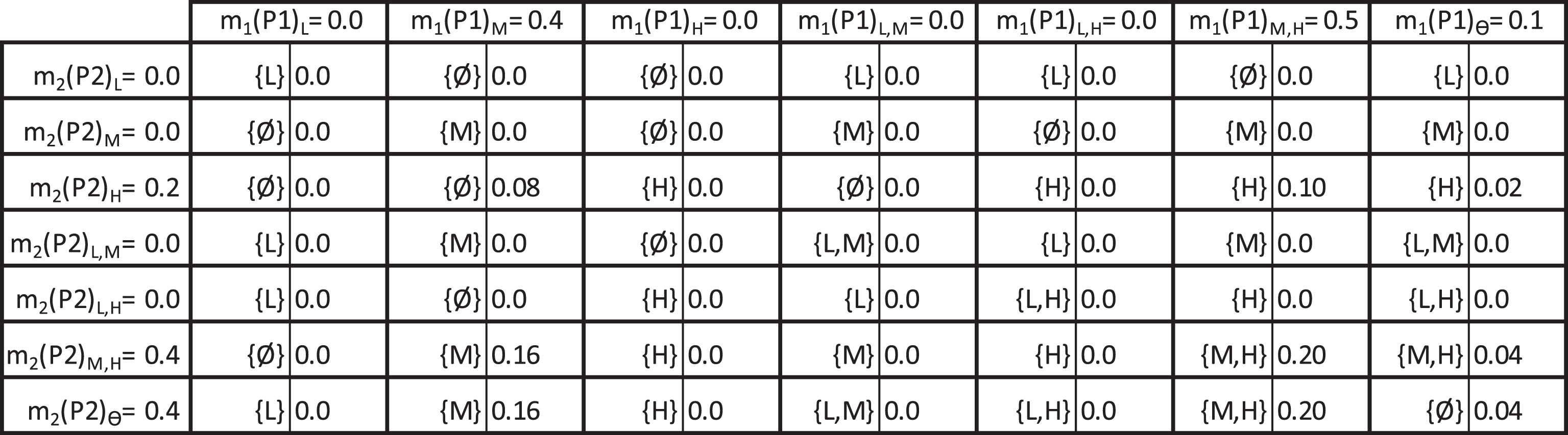
Condition states combinations based on D-S rule of combination.

From the above results, the degree of conflict where the intersection is deemed to be null (Ø) can be estimated as follows: K = 0.08+0.04 = 0.12. The normalization factor is 1 – k = 0.88. Finding the intersection of probabilities from the above combinations to produce each condition state by applying Equation 13 yields:

M_1 - 2(P)_L = 0.0; M_1 - 2(P)_M = (0.16+0.16)/0.88 = 0.36; M_1 - 2(P)_H = (0.1+0.02)/0.88 = 0.13;

M_1 - 2(P)_L,M = 0.0; M_1 - 2(P)_L,H = 0.0; M_1 - 2(P)_M,H = (0.2+0.2+0.04)/0.88 = 0.50; M1-2(P)θ= 0.04/0.88 = 0.04.

It can be concluded that based on the evidence from the two bridges where only routine maintenance was performed, the transition probability of going from Excellent to Good condition state can be rated as moderate with 36% belief, or moderate-high with 50% belief. The characteristics of each rating are as follow:

{M}: belief = 0.36, plausibility = 0.64 and belief interval [0.36,0.64]

{M,H}: belief = 0.50, plausibility = 0.50 and belief interval [0.50,0.50]

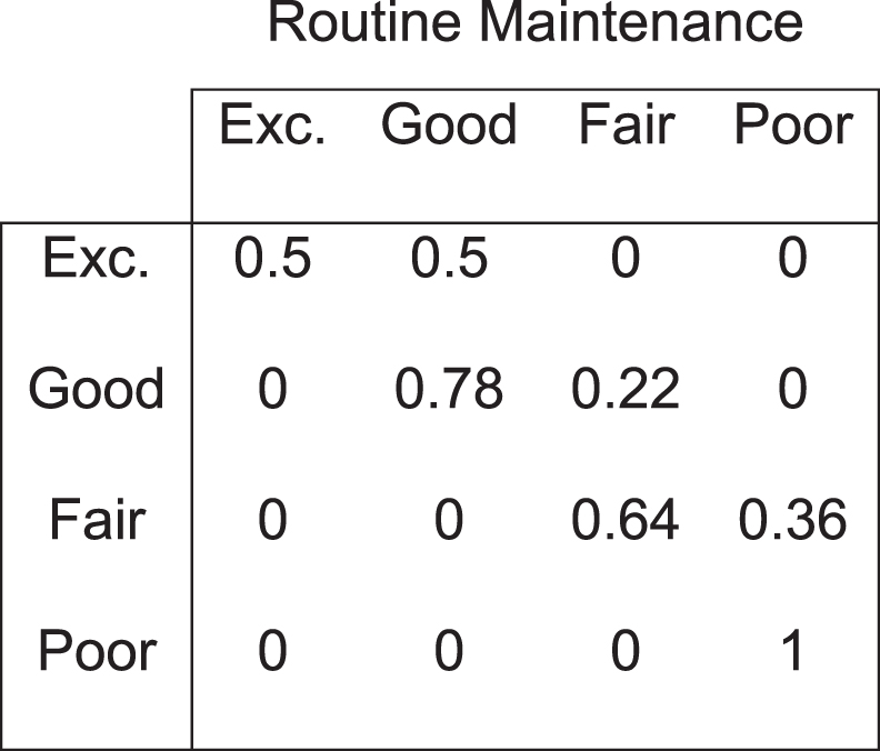
The same procedure is applied to elicit the engineer’s judgment on the possibility of transition from Good to Fair and from Fair to Poor condition states. The initial assessments are based on evidence from inspection reports, and the assessments can be refined as more evidence on the behavior of the deterioration process becomes available. Once the bridge element deteriorates to the Poor condition state, it will remain in that state as this is the worst condition that the element can reach. Transition probabilities can be assembled in a transition probability matrix as shown in Fig. 3.

Fig.3

Transition probabilities obtained based on expert judgment elicitation.

Abu Dabous et al. [1] used Monte-Carlo simulation to develop stochastic condition assessment of the bridge elements by quantifying the probability that the bridge element to be in each condition state. For instance, the condition probabilities of the bridge element are given by the following rating:

{(Excellent,10.96%),(Good,15.99%),(Fair,70.70%),(Poor,2.35%)}

The condition forecast of the bridge deck after one transition period can be estimated by multiplying the current condition vector by the transition probability (Equation 1) as follows:

		Exc.	Good	Fair	Poor
[10.96% 15.99% 70.70% 2.35%]×	Exc.	0.5	0.5	0	0
	Good	0	0.78	0.22	0
	Fair	0	0	0.64	0.36
	Poor	0	0	0	1

= [(Excellent,5.48%) (Good,17.95%) (Fair,48.77%) (Poor,27.80%)]

and then after two transition periods:

= [(Excellent,2.74%) (Good,16.74%) (Fair,35.16%) (Poor,45.36%)]

In this case study, the judgments are provided based on evidence collected from two bridges and have been quantified into belief percentages reflecting the transition probability of the bridge element under consideration. As more data and new evidence becomes available from additional bridges, the theory of evidence can combine the new information and update the transition probability assessment. The formulated transition probabilities are reviewed by the expert and found to be adequate to model the bridge deterioration process. The produced transition probabilities are used along with the condition ratings to forecast the condition of the bridge element after any number of transition periods. The analysis demonstrated the rate of deterioration impact on the condition forecast and showed how the element condition drops from the higher condition state to the lower ones.

6 Summary and conclusion

Estimating transition probabilities through analyzing available inspection data can be inadequate especially when inspection data is limited, when bridge inspection is done over time intervals different than the targeted transition period, and when inspection data relevant to advanced deterioration is not available. The other alternative is to estimate transition probabilities through expert judgment elicitation. The Dempster-Shafer theory of evidence is introduced to the area of bridge deterioration modeling as an innovative methodology to facilitate assessing expert judgments and to estimate deterioration transition probability. The application of the theory is demonstrated with a case example. The theory of evidence can efficiently deal with the difficulties related to subjective expert assessment of transition probabilities based on available limited data and can be applied when limited inspection data is available. The theory can assess the expert judgment and can refine assessment if additional evidence becomes available with time. The proposed approach in this paper is validated with one case study based on inspection records collected from two bridges. Further validation is recommended by applying the approach on more bridges to verify the performance of the theory of evidence while updating the transition probabilities as more evidence becomes available. Expert judgment elicitation to estimate deterioration transition probabilities has not received enough attention in the area of bridge deterioration modeling. Future research can compare transition probabilities obtained using statistical with probabilities estimated using judgment elicitation through the theory of evidence. Further studies can assess integrating results obtained from statistical analysis and expert judgment elicitation to produce more accurate deterioration models. Transition probabilities can be estimated based on specific bridge network inspection data and refined based on bridge engineers and managers inputs. Further, the theory of evidence implementation in the area of bridge management decision making can be investigated in the future.

References

Abu Dabous

, Alkass

, Zaki

. A probabilistic methodology for bridge deck condition assessment. Bridge Structures. 2008;4(1):49–56.

Alim

. Application of Dempster-Shafer theory for interpretation of seismicparameters. Journal of Structural Engineering. 1988;114(9):2070–84. ASCE.

AASHTO. Guidelines for bridge management systems. American Association of State Highway and Transportation Officials. 1993.

Bao

, Li

, An

, Ou

. Dempster-Shafer evidence theory approach to structural damage detection. 2012;11(1):13–26.

Cooke

, Goossens

LHJ

. Expert judgement elicitation for risk assessments of critical infrastructures. Journal of Risk Research. 2004;7(6):643–56.

Dempster

. A generalisation of Bayesian inference. Journal of Royal Statistical Society. 1968;Series B30:205–47.

Ellis

, Thompson

, Gagnon

, Richard

. Design and implementation of a new bridge management system for the Quebec Ministry of Transport. International Bridge and Structure Management. 10th International Conference on Bridge and Structure Management, Buffalo, IBSMC08-034. 2008:77–86.

FHWA. Transportation asset management case studies: Bridge management experience of California, Florida and South Dakota. U.S. Department of Transportation, Office of Engineering, Federal Highway Administration. 2005.

Frangopol

, Liu

. Bridge management based on multiple-objective optimization. Proceedings of the 5th International Conference on Bridge Management, Bridge Management 5: Inspection, Maintenance, Assessment and Repair, 2005.

10.

Golabi

, Shepard

. Pontis: A System for maintenance optimization and improvement of US bridge networks. Interfaces. 1997;27(1):71–88.

11.

Gucunski

, Pailes

, Kim

, Azari

, Dinh

. Capture and quantification of deterioration progression in concrete bridge decks through periodical NDE surveys. Journal of Infrastructure Systems. 2016:B4016005.

12.

Hajdin

, Peeters

. Bridging data voids: Advanced statistical methods for bridge management in KUBA. International Bridge and Structure Management: Tenth International Conference on Bridge and Structure Management, Buffalo, IBSMC08-027. 2008.

13.

Hawk

, Small

. The BRIDGIT bridge management system. Structural Engineering International. 1998;8(4):309–14.

14.

Huang

, Liu

, Sun

. A pavement crack detection method combining 2D with 3D information based on Dempster-Shafer theory. Computer-Aided Civil and Infrastructure Engineering. 2014;29(4):299–313.

15.

Jiang

, Satio

, Sinha

. Bridge performance prediction model using the Markov chain. Transportation Research Record. 1988;1180:25–32.

16.

Kallen

, Van Noortwijk

. A study towards the application of Markovian deterioration processes for bridge maintenance modelling in the Netherlands. Advances in Safety and Reliability, Proceedings of ESREL 2005 – European Safety and Reliability Conference, Tri City (Gdynia-Sopot-Gdansk), Poland. 2005

17.

Kyburg

. Bayesian and non-Bayesian evidential updating. Artificial Intelligence. 1987;31(3):271–93.

18.

Mašović

, Hajdin

. Modelling of bridge elements deterioration for Serbian bridge inventory. Structure and Infrastructure Engineering. 2014;10(8):976–87.

19.

Morcous

. Performance prediction of bridge deck systems using Markov chains. Journal of performance of Constructed Facilities. 2006;20(2):146–55.

20.

Morcous

, Lounis

. Maintenance optimization of infrastructure networks using genetic algorithms. Automation in Construction. 2005;14(1):129–42.

21.

Morcous

, Lounis

, Mirza

. Identification of environmental categories for Markovian deterioration models of bridge decks. Journal of Bridge Engineering. 2003;8(6):353–61. ASCE.

22.

OSIM. Ontario structure inspection manual. Ontario Ministry of Transportation, Structural Office, Bridge Management Section, Ontario, Canada. 2000.

23.

Sadiq

, Kleiner

, Rajani

. Estimating risk of contaminant intrusion in water distribution networks using Dempster-Shafer theory of evidence. Civil Engineering and Environmental Systems. 2006;23(3):129–41.

24.

Sadiq

, Rodriguez

. Interpreting drinking water quality in the distribution system using Dempster-Shafer theory of evidence. Chemosphere. 2005;59(2):177–88.

25.

Shafer

. A Mathematical theory of evidence. Princeton University Press, Princeton, NJ, USA. 1976.

26.

Thompson

, Merlo

, Kerr

, Cheetham

, Ellis

. The new Ontario bridge management system. Eighth TRB international bridge management conference, Denver, Colorado, USA. 1999.

27.

Thompson

, Shepard

. Pontis. Transportation Research Board, Washington, D.C., Transportation Research Circular, 324. 1994.

28.

Zargar

, Sadiq

, Naser

, Khan

, Neumann

. Dempster-Shafer theory for handling conflict in hydrological data: Case of snow water equivalent. Journal of Computing in Civil Engineering. 2012;26(3):434–47.

Assessing transition probability of bridge deterioration using Dempster–Shafer theory of evidence

Abstract

Keywords

1 Introduction

2 Research objective and methodology

3 Transition probability

4.1 Dempster–Shafer theory

4.2 Application of Dempster–Shafer theory

4.2.1 Basic probability assignment

References