Drive-by bridge damage detection using non-specialized instrumented vehicle

Abstract

Bridge structures are subject to continuous degradation, which requires an ongoing screening to give an early warning if the bridge becomes unsafe. In recent years, many authors have investigated a shift of the instrumentation from the bridge to a passing vehicle to collect indirect measurements for the bridge responses. This approach is known by ‘drive-by’ bridge inspection. This paper introduces a new method in the drive-by bridge inspection concept which employs acceleration measurements of a non-specialized vehicle to identify the change in the bridge responses due to structural damage. Two damage indices are included in the study, the vehicle acceleration spectra and the change in the bridge displacement. The paper will use an explicit approach for solving the Vehicle-Bridge Interaction (VBI) problem to give a more accurate representation of the truck/bridge interaction. The VBI problem will be solved using LS-Dyna Finite Element Analysis (FEA) program. The bridge is represented by discretized one-dimensional (1D) FE beam elements, and by discretized two-dimensional (2D) plate bending elements. Damage is defined in this study as a change in the damping ratio and/or gradual decrease in structure stiffness. Two vehicle models are used in the study, the two-degree-of-freedom quarter car model and the four-degree-of-freedom half car model. Both smooth and rough profiles are considered in the study.

Keywords

Bridge drive-by indirect monitoring SHM health monitoring vehicle

1 Introduction

Bridges are an integral part of transportation networks, and their strength degrades with time due to environmental effects and increased traffic loads. In the United States, there are about 66,405 structurally defective bridges, which is more than 11% of the total number of bridges [1]. The observation above raises questions regarding transportation network safety, which highlights the importance of structural health monitoring for bridges. As well as visual inspection, monitoring has for many years been based on the ‘Sensor Base Monitoring’ techniques where the bridge is instrumented with different types of sensors that observe any change in its responses [2 –4]. This type of monitoring is costly; furthermore, it limits the number of inspected bridges. Recently, some authors have shifted the instrumentation from the bridge to a passing vehicle which makes the concept far more cost effective than traditional monitoring techniques. This technique is known as ‘Drive-by Bridge Inspection’ [5]. McGetrick et al. studied the feasibility of using the axle acceleration signal of an instrumented truck in identifying the bridge damage [6, 7]. In their study, they used the change in the acceleration Power Spectral Density (PSD) as a bridge damage indicator. The approach shows promising results in the absence of the road roughness heights. On the other hand, when the road roughness is added to the Vehicle-Bridge Interaction (VBI) problem, the vehicle bouncing and pitching frequencies dominate the acceleration spectra. This is because the road roughness excites the vehicle more than the bridge does. Therefore, the bridge frequencies, and hence the change in the frequency due to structural degradation are totally masked by the vehicle excitation. Kim et al. [8], experimentally validated the drive-by inspection approach utilizing a scaled laboratory test. The authors introduced three levels of screening for the bridge. The first level focuses on monitoring the changes in the acceleration spectra due to structural damage. The second level monitors the changes of the modal damping constant and modal circular frequencies of the VBI system. Levels 1 and 2 utilize only the vehicle measurements to estimate the damage. The third level employs both the vehicle and the bridge measurements to estimate the Element Stiffness Index (ESI). The results of the first two screening levels show that the approach gives good results for low speeds, while for higher speeds the responses are masked by the profile effect on the vehicle. The third screening level shows robust damage identification. However, it requires information from the vehicle and the bridge. Keenahan et al. [9] in 2013 proposed an intensive investigation, using the acceleration spectra as a damage indicator. The authors represented the inspection vehicle using separate quarter car models, then as a continuous truck trailer model. They found that the PSD for the axle acceleration signals can be utilized successfully in identifying bridge damage in the presence of road roughness if the accelerations of two consecutive axles are subtracted before transferring from the time domain to the frequency domain. However, their approach is only shown to work for damage represented by an increase in the damping ratio. In 2012, González et al. [10] built an algorithm that identifies the bridge damping using the truck acceleration histories. The algorithm uses a half car model with two axles. The algorithm identifies the damping by minimizing the error in the difference between the front and the rear axle profiles. The algorithm is shown to be insensitive to random noise and modeling inaccuracy. Recently, OBrien and Keenahan [11] developed the ‘Apparent Profile’ as a bridge damage indicator. The ‘Apparent Profile’ denotes the sum of the road roughness heights and the bridge displacements. They calculated the Apparent Profile using a notional Traffic Speed Deflectometer truck which measures the relative displacement history between a horizontal beam in the truck and the road surface. Using a Matlab algorithm, the authors generated n random profiles in the first sample using the Cross-Entropy optimization scheme and evaluate the corresponding relative displacement history between the theoretical vehicle and the generated road profiles using an implicit VBI Matlab algorithm. The algorithm then evaluates the difference between the measured and calculated relative displacement histories. The Cross-Entropy algorithm will use the data of the first generation of solutions to generate another n profiles, seeking the profile that minimizes the difference between the measured and calculated relative displacement histories. The process is repeated until the objective function converges when the difference in two successive samples is less than 0.005%. The authors validated the Apparent Profile for different damage representations, and it is shown to be very sensitive to bridge damage, even for small changes in the bridge stiffness.

This paper extends the idea, by studying the feasibility of using a non-specialized vehicle instrumented with accelerometers, instead of the Traffic Speed Deflectometer, to detect bridge damage. Two damage indicators are investigated in this paper, the Power Spectral Density (PSD) of the vertical axle acceleration and the back calculated ‘Apparent Profile’ (AP). Many authors have introduced the acceleration spectra as an indirect damage index for the bridge structures. However, the solver used for the VBI problem was an implicit one. Herein, the LS-Dyna Finite Element Analysis (FEA) [12] explicit solver is used for the VBI problem to have more reliable results for the acceleration histories. The method presented in this paper has the advantage of using a regular truck instrumented with conventional accelerometers instead of the highly specialized Traffic Speed Deflectometer truck. The study will be carried out on one-dimensional (1D), and two-dimensional (2D) bridge models. Damage is represented as a loss of structural stiffness and change in damping ratio.

2 Vehicle and bridge properties

Two different models are used for the vehicle. First, the theoretical quarter car model (Fig. 1) with two degrees of freedom, which allows for axle hop and body mass bouncing. The second model is a theoretical half car model (Fig. 2) with four degrees of freedom, which allows for axle hops, body mass bouncing, and body mass pitch rotation. The body mass is represented in LS-Dyna as a rigid bar with mass moment of inertia I_s, to account for the body mass pitch rotation. The distance between each axle and the body mass center of gravity is D₁ and D₂ for axles ‘1’ and ‘2’ respectively. The properties of the half car and the quarter car are listed in Tables 1 and 2 and are based on the work done by Cebon [13] and Harris et al. [14].

Fig.1

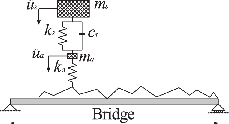
Theoretical quarter car model.

Fig.2

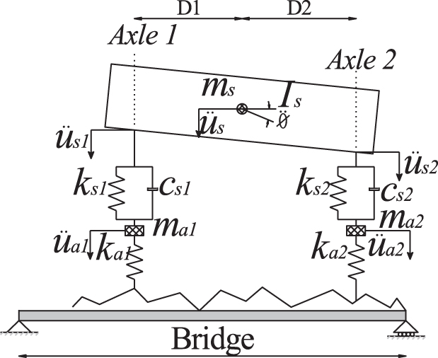
Theoretical half car model.

Table 1

Properties of quarter car model

Property	Unit	Symbol	Quarter
			Car Model
Body Mass	kg	m_s	17300
Axle Mass	kg	m_a	700
Suspension Stiffness	N/m	k_s	4×10⁵
Suspension Damping	N.s/m	c_s	10×10³
Tire Stiffness	N/m	k_a	1.75×10⁶
Body Mass Frequency of Vibration	Hz	f_bounce	0.69
Axle Mass Frequency of Vibration	Hz	f_axle	8.8

Table 2

Properties of quarter car model

Property	Unit	Symbol	Quarter Car Model
Body Mass	kg	m_s	16600
Axle Mass	kg	m_a1,m_a2	700
Suspension Stiffness	N/m	k_s1,k_s1	4×10⁵
Suspension Damping	N.s/m	c_s1,c_s2	10×10³
Tire Stiffness	N/m	k_a1,k_a2	1.75×10⁶
Mass Moment of Inertia	kg.m²	I_s	95765
Distance of Axle to Center of Gravity	m	D₁,D₂	2.375
Body Mass Frequency of Vibration	Hz	f_bounce	1
		f_pitch	1
Axle Mass Frequency of Vibration	Hz	f_axle1, f_axle2	8.8

Three simply supported bridges are studied with 10 m, 20 m, and 30 m spans. An eigenvalue analysis is performed to extract the bridges’ fundamental frequencies using LS-Dyna. The bridges have an elastic modulus of E_c = 3.5×10¹⁰ N/m² and a density of γ= 2400 kg/m³. The properties of the studied bridges are listed in Table 3 and are based upon the work of Elfayoumy [15].

Table 3

Bridge properties

Span (m)	First Natural	2nd Moment of Area Around the	Section Area
	Frequency (Hz)	Horizontal Axis of the Cross	(m²)
		Section (m⁴)
10	8.75	0.0434	2.04
20	3.77	0.1518	2.40
30	2.39	0.3534	2.76

The bridges are represented in the program using one-dimensional (1D) Belytschko-Schwer beam elements. The bridges are divided into small segments of 0.5 m length, and the elements have a constant rectangular cross section giving the same properties listed in Table 3.

The crossing of the vehicle over the bridge is modeled using the LS-Dyna FEA program. Both quarter and half car models move with a constant speed of 25 m/s (90 km/hr) over a 200 m approach distance, to eliminate the effect of the free vibration at the initiation of the simulation, followed by the bridge. The quarter car is modeled moving over both smooth and rough profiles, while rough profile only is used for the half car model for the sake of brevity in the paper.

3 Apparent profile calculation

While the vehicle crosses the bridge, it is in equilibrium with the reaction of the road on the vehicle tires at each time step. Therefore, if the road reaction history at the contact point is known, and the vehicles are modeled without the bridge as shown in Fig. 3, the application of the road reaction force history at the vehicle tires will excite it in the same way it was excited by the bridge. The contact node will also move to mimic the profile that produces this force history. The AP is the sum of the road roughness heights plus the bridge displacement which is the contact node displacement history. Therefore, using the vehicle acceleration histories, the road reaction force history on the vehicle tires can be found, and the AP is found by applying the forces to the vehicle model.

Fig.3

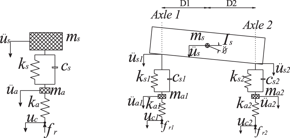
Apparent profile calculation model.

The instrumented inspection truck will cross the bridge under its current structural health condition. The collected data from the truck will then be used to evaluate the AP for the healthy/current state of the bridge. After a period of time, the structural elements of the bridge will have some level of degradation. The inspection vehicle will be used to cross over the bridge after it has deteriorated to calculate the AP for the damage state. The difference between the two APs will then be used to estimate the level of bridge degradation.

The evaluation of the AP is based on re-simulating the vehicle crossing the bridge without including the bridge in the problem as discussed before. The idea builds upon stabilizing the vehicle model by replacing the road-bridge system with its reaction on the vehicle at the moment when the vehicle exists on the bridge. The calculation of the road reaction force histories from the instrumented truck is a key element in back figuring the AP. The road reaction can be calculated employing Equation 1 for the quarter car model and Equation 2 for the half car model:

$f_{r_{i}} = - [m_{v}] {{\ddot{u}}_{v}}_{i} 〈 1 〉$ (1) ${\begin{matrix} f_{r 1} \\ f_{r 2} \end{matrix}}_{i} = - [\begin{matrix} \begin{matrix} 1 & 0 & D_{2} & 1 / D_{1} \end{matrix} \\ \begin{matrix} 0 & 1 & D_{1} & - 1 / D_{2} \end{matrix} \end{matrix}] [m_{v}] {{\ddot{u}}_{v}}_{i}$ (2) where, [m_v] is the vehicle mass matrix, ${{\ddot{u}}_{v}}_{i}$ is the acceleration vector for the vehicle degrees of freedom at time step i.f_{r
_i} is the road reaction force at step i for the quarter car model. f_{r1_i} and f_{r2_i} are the road reactions on axles 1 and 2, respectively, at step i. The road reaction force (or the tire force) history/histories will be applied to the modified vehicle model to evaluate the AP (Fig. 3). For the quarter car model, the model has one more degree of freedom to account for the contact node displacement history u_c, while the half car model will have two more degrees of freedom for the front and rear contact nodes u_c1, u_c2. The AP can be calculated by solving the vehicle equation of motion independently from the bridge as shown in Equations 3 and 4 for the quarter and half car models respectively.

$\begin{matrix} {[m_{v}]}^{'} {\begin{matrix} {{\ddot{u}}_{v}} \\ {\ddot{u}}_{c} \end{matrix}}_{i} + {[c_{v}]}^{'} {\begin{matrix} {{\dot{u}}_{v}} \\ {\dot{u}}_{c} \end{matrix}}_{i} \\ + {[k_{v}]}^{'} {\begin{matrix} {u_{v}} \\ u_{c} \end{matrix}}_{i} = {\begin{matrix} {0} \\ f_{r} \end{matrix}}_{i} \end{matrix}$ (3)

$\begin{matrix} {[m_{v}]}^{'} {\begin{matrix} {{\ddot{u}}_{v}} \\ {\ddot{u}}_{c 1} \\ {\ddot{u}}_{c 2} \end{matrix}}_{i} + {[c_{v}]}^{'} {\begin{matrix} {{\dot{u}}_{v}} \\ {\dot{u}}_{c 1} \\ {\dot{u}}_{c 2} \end{matrix}}_{i} \\ + {[k_{v}]}^{'} {\begin{matrix} {u_{v}} \\ u_{c 1} \\ u_{c 2} \end{matrix}}_{i} = {\begin{matrix} {0} \\ f_{r 1} \\ f_{r 2} \end{matrix}}_{i} \end{matrix}$ (4) where [m_v] ′, [c_v] ′ and [k_v] ′ are the modified vehicle mass, damping and stiffness matrices. The equation is solved using the LS-Dyna explicit solver by modeling the vehicle only and applying the forces at the contact nodes. The output will be the contact node displacement history u_c, u_c1,2, which is the AP.

The approach mentioned above can be easily extended in the field by instrumenting an inspection truck with accelerometers to measure the axle masses, and the body mass vertical acceleration histories and a gyroscopic accelerometer to measure the body mass pitching acceleration. The body mass center location can be easily found by applying equilibrium to the axle weights that can be measured in the field with Wheel Load Scale pads.

4 Results of one-dimensional bridge model

4.1 Quarter car model

4.1.1 In the absence of road roughness

The quarter car model will cross over the approach distance followed by the damaged bridge to investigate the adopted monitoring indices, i.e. the acceleration spectra, and the AP. Damage is represented either as a change in bridge damping as recommended by Curadelli et al. [16], or as a gradual decrease in structural stiffness as adopted by Sinha et al. [17]. In the latter damage model [17], the crack is assumed to cause a loss in stiffness over a region three times the beam depth, varying linearly from a maximum at the crack location. The damage is defined as the ratio of crack depth to overall beam depth; thus 20% damage implies that the crack depth is 20% of the beam depth. The Sinha damage model [17] has been established for different end support conditions for simple metallic beams. Therefore it does not guarantee an accurate representation of the damage in a real life situation. However, the model, as introduced in previous research work [9, 11], will be used in this paper to investigate the feasibility of the approach. A further investigation is required to address adopted damage representations for different bridges (i.e. concrete, steel and hybrid systems) to allow for a robust conclusion about the feasibility of the approach in real-life situations. Unless otherwise noted, the damage will be located at 2/3 of the bridge span from the approaching side.

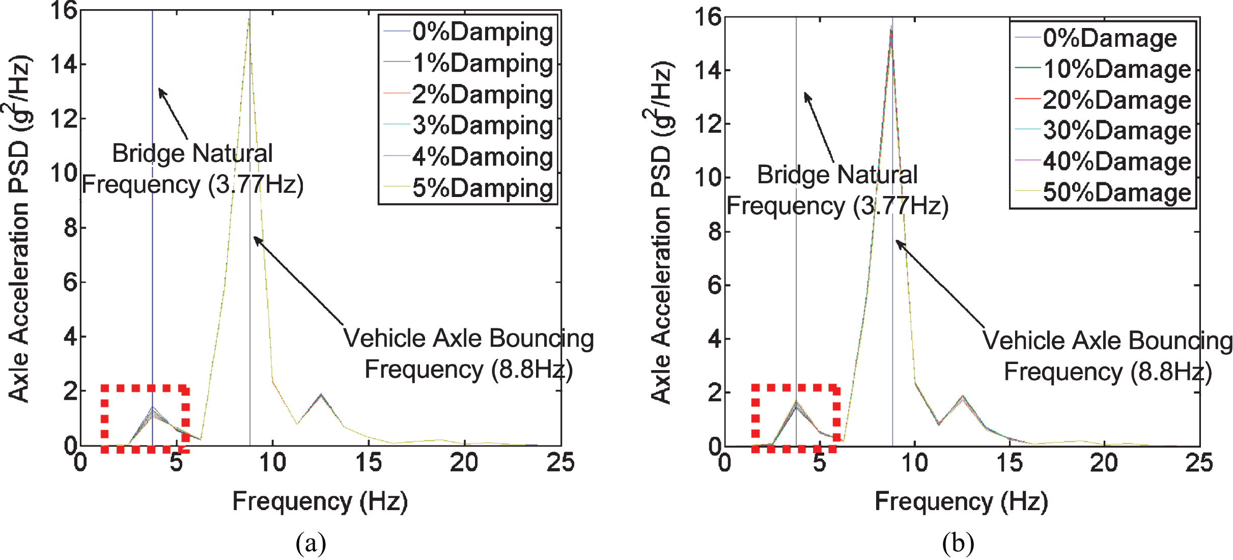
Herein, the quarter car crosses the approach distance followed by the 10 m simply supported bridge with a smooth profile. This is repeated twelve times, once for each damping ratio (from 0% to 5%), then for each crack depth (from 0% to 50%). The quarter car axle acceleration is transformed from the time domain to the frequency domain using the Fast Fourier Transform (FFT). The sampling rate of the data is 1000 Hz, the length of the acceleration signal is 400 samples, and the frequency resolution is 2.5 Hz. The six different Power Spectral Density (PSD) curves are plotted on the same graph for each damage criterion, with frequency on the x-axis (Fig. 5). A peak in the acceleration spectra can be observed near the bridge frequency (8.75 Hz) for both damage criteria. However, for a change in the damping ratios, a decrease in the PSD peak can be observed as the bridge damping increases. For loss in stiffness, however, almost no change in the PSD peak is evident. The process has been repeated for the 20 m and 30 m bridges, and similar results were obtained.

Fig.4

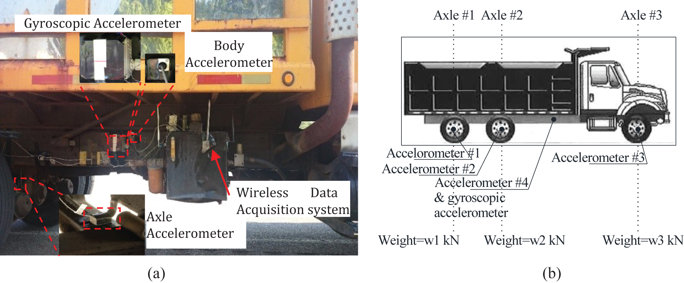
Inspection vehicle instrumentation (a) Type of sensors (b) Instrumentation configuration.

Fig.5

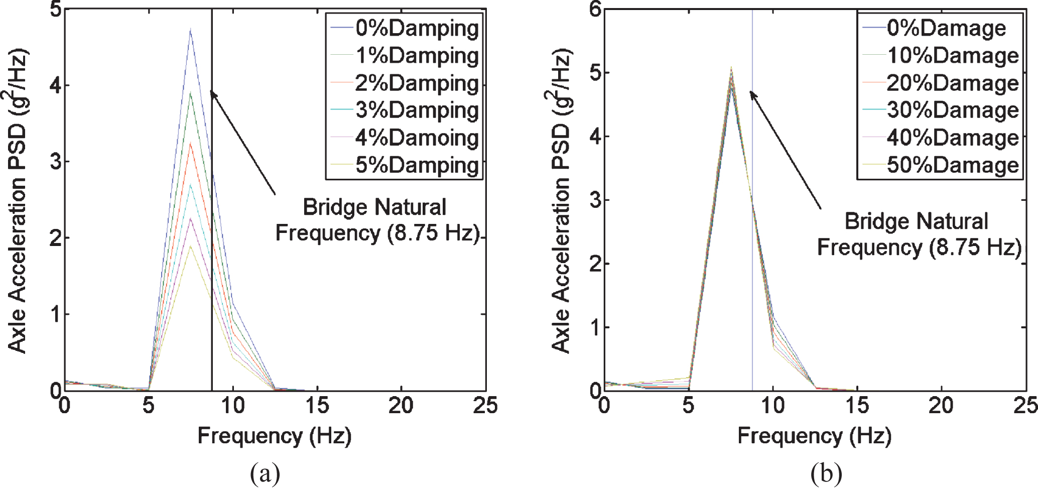
PSD for axle acceleration for 10 m bridge with no roughness (a) Damage as a change in bridge damping ratio (b) Damage as a change in stiffness.

The quarter car acceleration histories are measured from the LS-Dyna FEA model, then the accelerations are used in Equation 1 to evaluate the road reaction force history, f_ri. The force is then applied as an input to the modified quarter car vehicle model to calculate the contact node displacement history, u_c, or the AP. The process is repeated for the six different damping values and two damage levels. The resulting APs are shown in Fig. 6, where modest change can be observed in the APs for both cases due to structural damage.

Fig.6

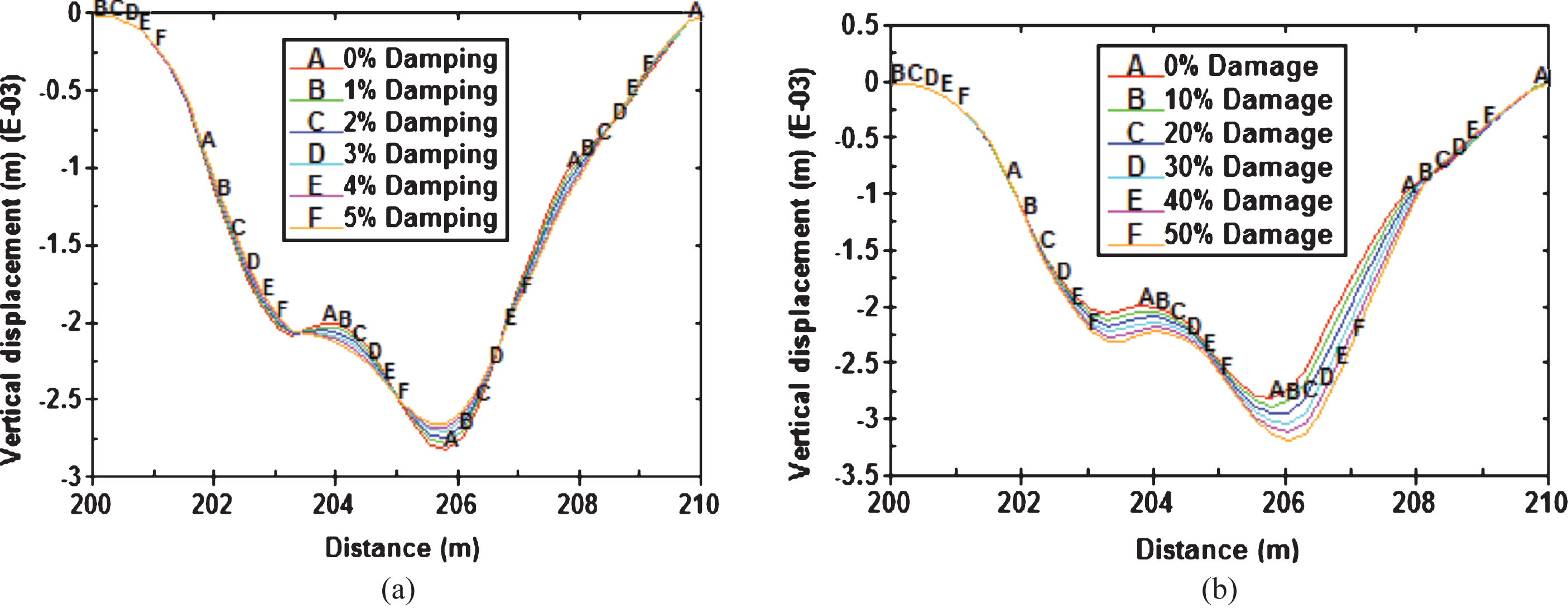
Apparent Profiles for 10 m bridge calculated from the quarter car model (a) Damage as a change in bridge damping ratios (b) Damage as a change in stiffness.

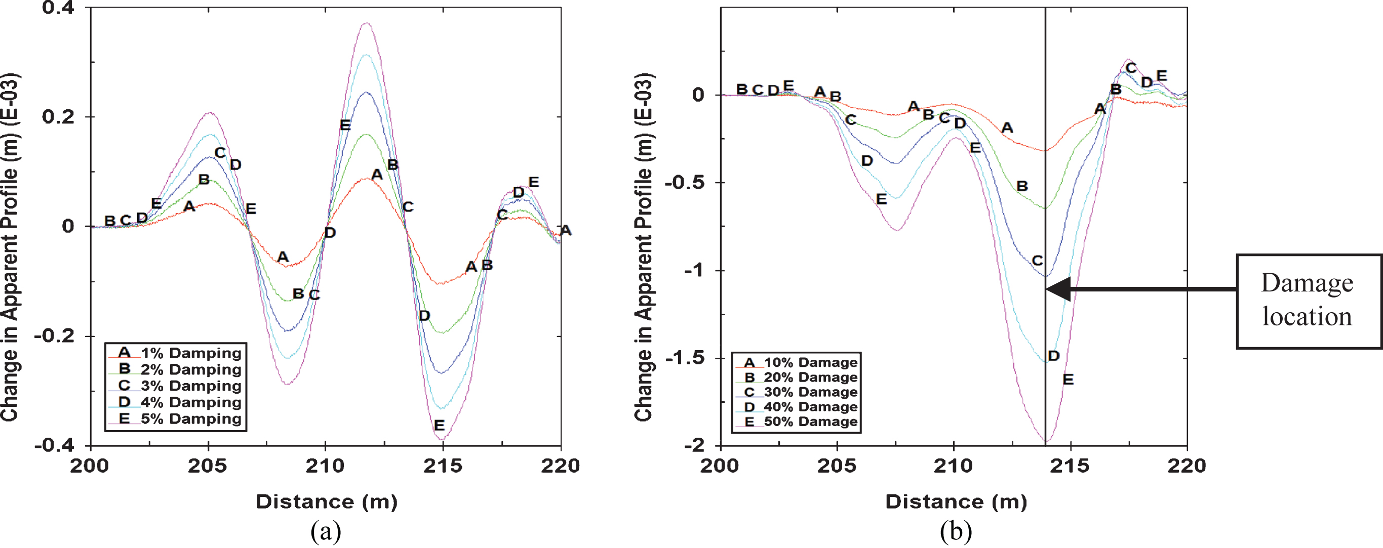
The APs will be subtracted from a baseline AP to track the change in the bridge displacement due to structural degradation. Herein, the baseline profile will be the AP^0 %, which in this case represents the AP of the first screening for the bridge with the inspection vehicle. The level of deviation from the baseline profile reflects the degree of structural degradation in the bridge. The changes in the APs are calculated by subtracting the APs from the baseline AP. The results are shown in Fig. 7 and, contrary to the acceleration spectra, they can be seen to be sensitive for the two damage representations. Similar results are found for the other two bridges.

Fig.7

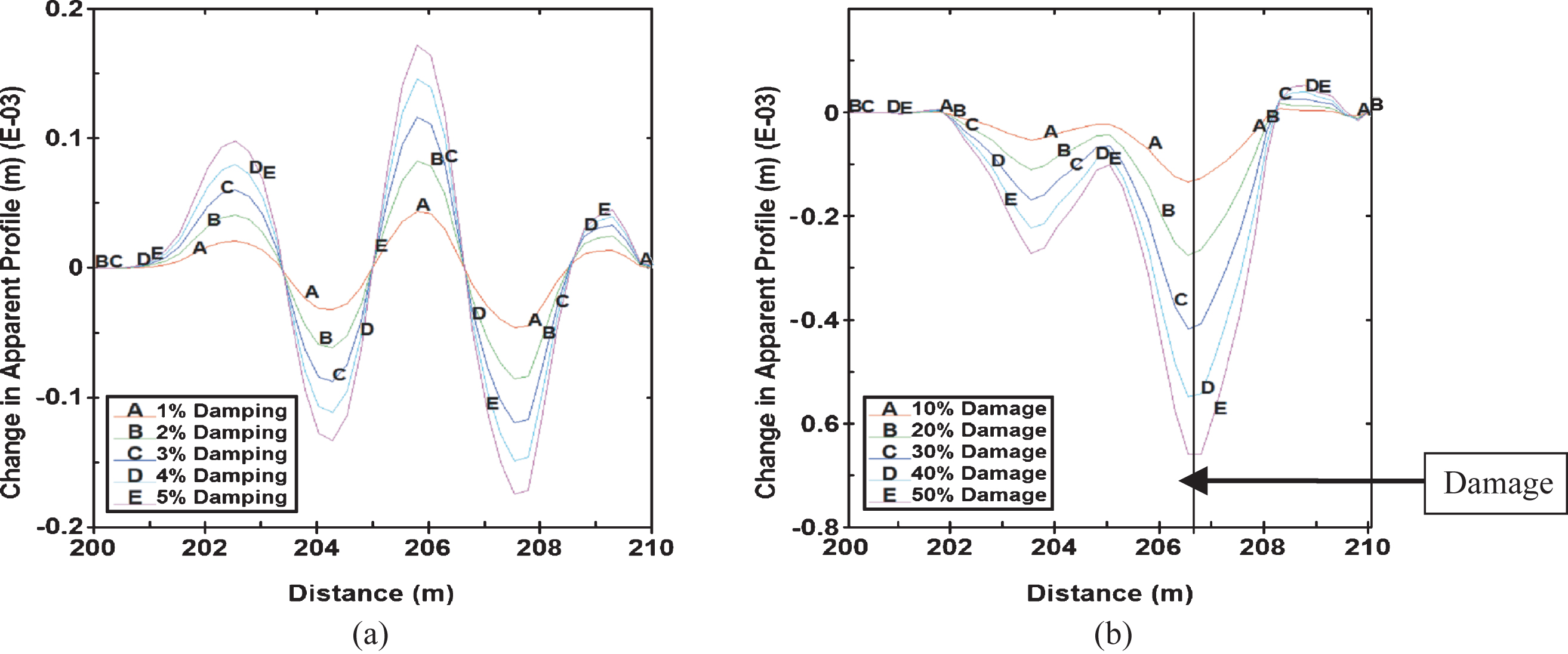
AP differences for the 10 m bridge (a) Damage as a change in bridge damping ratios (b) Damage as a change in stiffness.

The introduced method for calculating the AP is based upon solving the vehicle equation of motion for a set of time steps knowing the vehicle acceleration history. This gives the approach an advantage over the optimization approaches, where the number of data points is essential to estimate the APs accurately. Alternatively, it finds the exact value for the AP at each time step solving the vehicle equation of motion. This gives the approach a new degree of freedom regarding the required number of data points which is related to traveling time on the bridge and hence the driving speed. Therefore, the approach can work with different driving speeds. However, higher driving speeds are recommended to induce a significant level of deformation to observe the difference due to structural damage; if such damage exists.

4.1.2 In the presence of road roughness

In this section, a rough profile is included in the simulations. Two road profiles are randomly generated according to ISO-8608 [18], profile Class ‘A’ and profile Class ‘B’ as shown in Fig. 8.

Fig.8

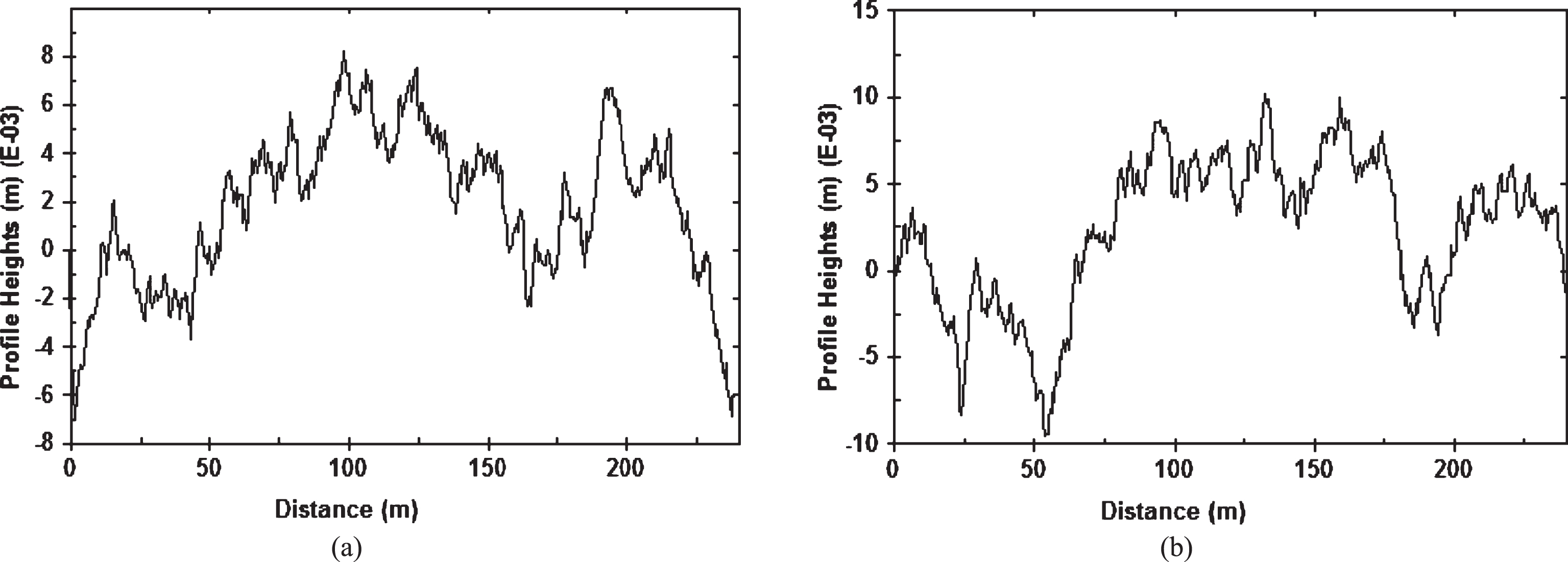
Road profile elevation versus distance (a) Road profile Class ‘A’ (b) Road profile Class ‘B’.

Herein, the results of the 20 m bridge are presented, and similar results are found for the 10 m and the 30 m bridges. The same two damage representations are included in this case. The acceleration spectra for the two cases are shown in Fig. 9. The results indicate that the vehicle frequencies dominate the spectrum; however, in contrast to previous studies [6 , 19], small variations in the PSD peaks are observed near the bridge frequency. This observation is due to the nature of the solver employed in this study. The LS-Dyna software solves the VBI problem utilizing an explicit analysis, which is more suitable for the nature of this problem. The VBI problems consider a time-dependent scenario where the bridge is highly excited due to the impact of the crossing vehicle. In contrast, the implicit solver is adequate for static or quasi-static problems. Thus, for the VBI simulations, the employment of the explicit solver will lead to a better estimation for the bridge and the vehicle responses, specifically, the vehicle acceleration.

Fig.9

PSD for axle acceleration for 20 m bridge with roughness Class ‘B’ (a) Damage as a change in bridge damping ratios (b) Damage as a change in stiffness.

The APs have been evaluated using the same process as before. Fig. 10 shows the difference between the APs for each damage level and both damage criteria. Comparing the Apparent Profile difference in Fig. 7 and Fig. 10, it can be seen that the road roughness has no effect on the change between the APs since the profile is removed in the subtraction process for the APs. It is noteworthy that the AP concept has been investigated, theoretically, assuming that the change in the road roughness with time is of insignificant order in comparison with the change in bridge displacement due to structural damage [11]. A further investigation is required to model the wearing of the road roughness with time and its impact on the AP approach.

Fig.10

Change in Apparent Profile for 20 m bridge with roughness Class ‘B’ (a) Damage as a change in bridge damping ratios (b) Damage as a change in stiffness.

4.2 Results of the half car model

The half car model constitutes a more representative model of the real life truck since it accounts for more degrees of freedom for the vehicle’s mechanical system. Keenahan et al. [9] recommended using the spectrum of the subtracted axle acceleration of a half car model with respect to the axle position (i.e. subtract the acceleration of the front axle from the rear axle acceleration when the rear axle reaches the front axle position). The authors claim that this process substantially eliminates the road roughness effect from the spectrum. However, the approach is only shown to work for damage as a change in damping. Herein the approach is going to be re-investigated using the explicit solver of the LS-Dyna program. As before, the half car crosses a 200 m approach distance followed by the 20 m simply supported bridge with road roughness Class ‘A’. The ‘subtracted’ axle acceleration is transformed from the time domain to the frequency domain to get the PSD. As shown in Fig. 11, the effect of the road roughness has been totally removed from the spectrum, and the damage has been clearly identified in the two cases.

Fig.11

PSD for subtracted axle acceleration for 20 m bridge with roughness Class ‘A’ (a) Damage as a change in bridge damping ratios (b) Damage as a change in stiffness.

The APs for the front and rear axles are calculated employing Eq. 2 and Eq. 4. The calculated profiles will not be subtracted from a baseline profile as introduced before. Alternatively, the profile under the front axle will be subtracted from the profile under the rear axle when the rear axle reaches the position of the front axle as illustrated in Eq. 5.

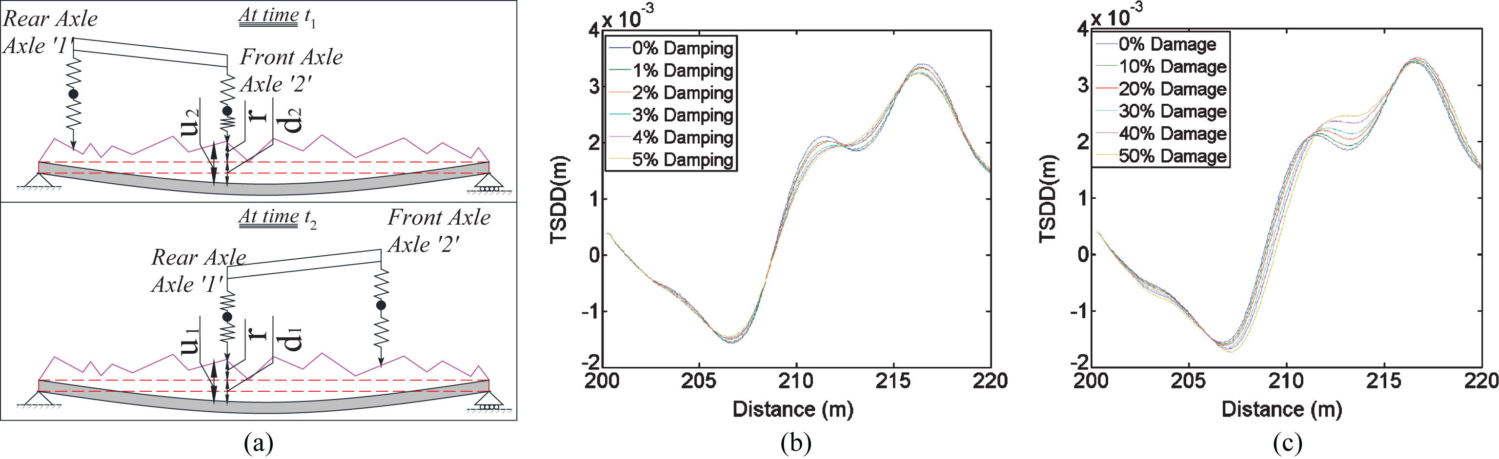
$\begin{matrix} u_{2 at t 2} - u_{1 at t 1} = (d_{2 at t 2} + r) - (d_{1 at t 1} + r) \\ = d_{2 at t 2} - d_{1 at t 1} \end{matrix}$ (5) where u₁ and u₂ are the total displacements under axles ‘1’ and ‘2’, respectively. The total displacement equals the summation of the road profile ‘r’ and the bridge displacement under the axle at that step. The subtraction of the two profiles will substantially remove the road roughness from the problem leaving only the Time Shifted Displacement Difference (TSDD) under axles ‘1’ and ‘2’. Fig. 12(a) illustrates the subtraction process. The TSDD for the two cases is shown in Figs. 12 (b) and (c).

Fig.12

Time Shifted Displacement Difference (a) Subtraction process to get the TSDD (b) TSDD for damage as a change in bridge damping ratios (b) TSDD for damage as a change in stiffness.

In a similar way to the AP, the TSDD will be subtracted from a baseline profile which will be the TSDD for 0% damage. The results are shown in Fig. 13. The change in the TSDD is shown to be quite sensitive to the bridge damage, for damage represented either as a change in bridge damping or as a loss in structural stiffness. Furthermore, change in the TSDD accurately identifies the damage location along the bridge as shown in the figure. Therefore the approach can be used for damage assessment and localization.

Fig.13

Time Shifted Displacement Difference Change for 20 m bridge with roughness Class ‘A’ (a) Damage as a change in bridge damping ratios (b) Damage as a change in stiffness.

5 Results of two-dimensional bridge model

This section for the first time extends the drive-by bridge inspection concept to two-dimensional problems. In this regard, the bridges are modeled using 1000 Belytschko-Tsay shell elements with five integration points per element. Only the change in the TSDD is investigated as a damage index in this section. Similarly, the half car will cross the approach distance before passing over the 10 m bridge. Roughness Class ‘A’ is used for this simulation. The half car model is transversely located at 0.6 m in from the bridge edge. Similarly, the damage is located at almost 2/3 of the bridge span. Figures 14 and 15 illustrate the half car model and the bridge in the LS-Dyna program. The truck acceleration histories are collected from the LS-Model then used to calculate the APs and hence the TSDD changes for the 10 m bridge as shown in Fig. 16. In a similar way to the one-dimensional model, the profiles is shown to be quite sensitive to structural damage.

Fig.14

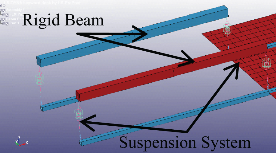
Half car model in LS-Dyna.

Fig.15

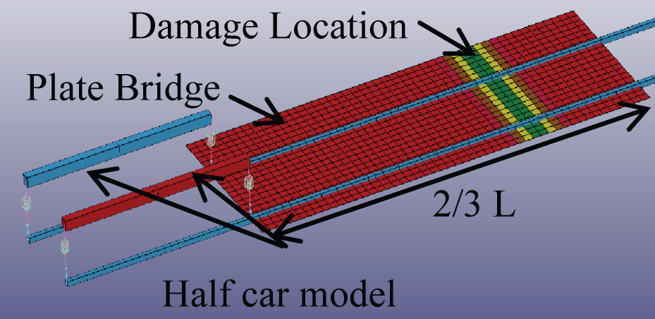
Two dimensional bridge model with damage crossing the whole cross-section.

Fig.16

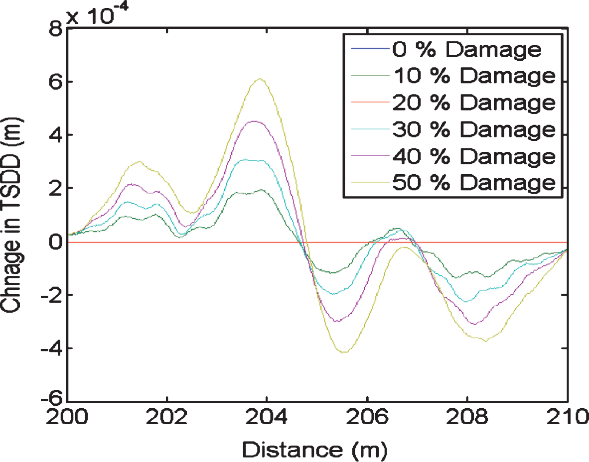
Time Shifted Displacement Difference Change for 2D 10 m bridge.

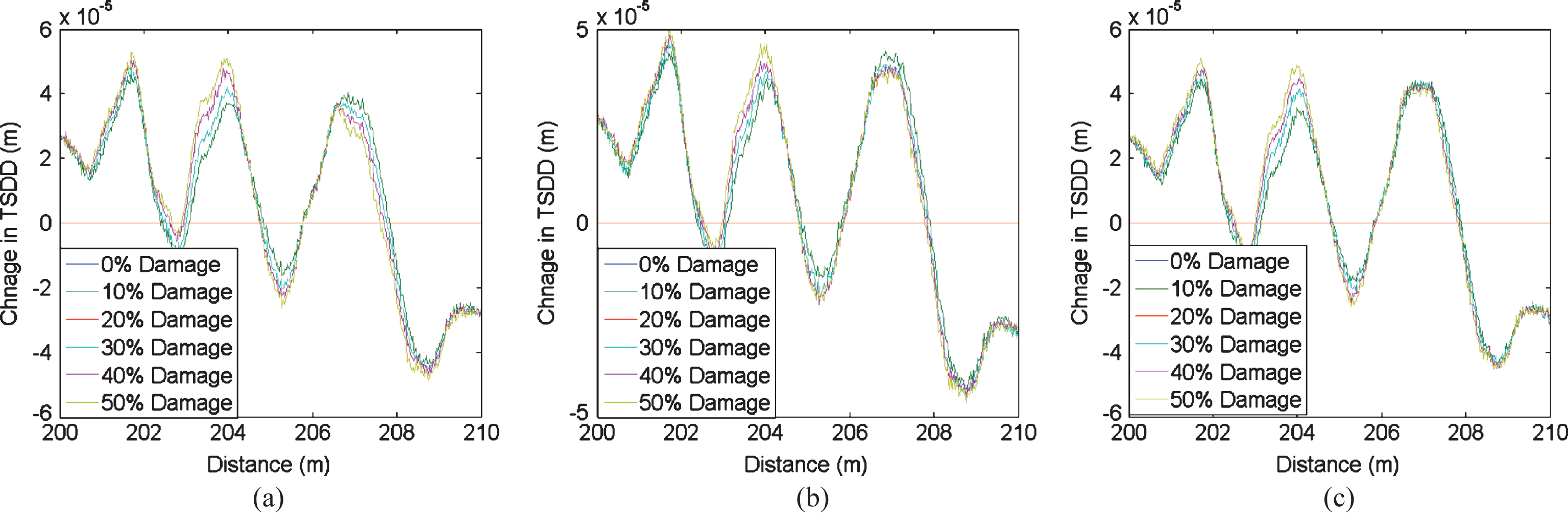
The sensitivity of the approach to the damage extent will be investigated by reducing the transverse crack width. First, the crack width will be reduced to one-third (1/3) of the bridge width as shown in Fig. 17. The damage will exist in the beginning at the initial 1/3 of the bridge width; then the damage will be transversely shifted to the mid third and finally to the last third. The TSDD changes for this case are illustrated in Fig. 18, indicating that the sensitivity to damage is reduced when compared with the crack crossing the full transverse width. However, still, the approach can identify the damage. The damage is reduced to one-tenth (1/10) of the bridge width, and similarly, the TSDD change is calculated. The results, illustrated in Fig. 19, show that reducing the damage extent reduces the sensitivity of the approach to damage. However, the use of a heavier truck may induce a considerable deformation that can be used to differentiate between the bridge responses under minor damages.

Fig.17

Damage location across the bridge: (a) first third, (b) mid third, and (c) last third.

Fig.18

Time Shifted Displacement Difference Change for 2D 10 where damage located at: (a) first third, (b) mid third (c) last third.

Fig.19

Time Shifted Displacement Difference Change for 2D 10 m where damage located at: (a) first 1/10, (b) mid 1/10, and (c) last 1/10.

6 Summary and conclusions

This paper introduces the use of a non-specialized vehicle for bridge damage identification using indirect measurements from the vehicle. The paper investigated two damage indices in this regard. The first index is the acceleration spectra of the axle acceleration which is shown to be totally masked by the vehicle frequencies in the presence of road roughness. This effect can be removed by subtracting the acceleration signal of the front and the rear axles with respect to the axles’ position on the road. The spectra of the subtracted signal show a proper identification for the damage, unlike the findings of previous studies. This is due to employing an explicit solver (LS-Dyna) instead of the implicit one for the VBI problem. The second index is the bridge ‘Apparent Profile’. The AP is shown to be quite sensitive to structural damage. The AP has been extended to evaluate the change in the Time Shifted Displacement Difference TSDD. The TSDD change has been investigated for different damage levels for one and two-dimensional problems and shows a considerable sensitivity to damage. This is with the exception of minor damage, where modest changes are observed in the TSDD curves. The advantage of switching to the TSDD is that it can be used as an input to an optimization scheme to estimate the current bridge health condition since the TSDD change for the 0% damage case can be evaluated using an equivalent finite element bridge model. On the other hand, the AP^0 % cannot be identified in field applications, since it requires updated information about the road roughness profile. In short, the AP concept can be used for monitoring the degradation, while the TSDD change can be used for structural health assessment. The approach considers normal operational environment concerning the wind speed and the temperature. The effect of those parameters on the approach sensitivity is still under investigation.

References

Davis

, Goldberg

, DeGood

, Donohue

, Corless

. The Fix We’re In For: The State of Our Nation’s Bridges 2013. FHWA.2013.

Chajes

, Shenton III

. Using diagnostic load tests for accurate load rating of typical bridges. Bridge Structures. 2006;2(1):13–23.

Sivakumar

, Sheikh Ibrahim

. Enhancement of bridge live loads using weigh-in-motion data. Bridge Structures. 2007;3(3-4):193–204.

Shoukry

, William

, Riad

, Luo

. Enhancement of bridge live loads based on West Virginia weigh-in-motion data. Bridge Structures. 2008;4(3-4):121–33.

Kim

, Kawatani

. Challenge for a drive-by bridge inspection. International Conference; 10th, Structural Safety and Reliability; Safety, Reliability and Risk of Structures, Infrastructures and Engineering Systems; ICOSSAR 2009; Osaka, Japan. 2009.

McGetrick

, González

, OBrien

. Theoretical investigation of the use of a moving vehicle to identify bridge dynamic parameters. Insight-Non-Destructive Testing and Condition Monitoring. 2009;51(8):433–8.

McGetrick

, González

, O’Brien

. Monitoring bridge dynamic behaviour using an instrumented two axle vehicle. Bridge and Infrastructure Research in Ireland 2010 (BRI 10), Cork, 2-3 September 2010; 2010: BCRI.

Kim

C-W

, Isemoto

, Toshinami

, Kawatani

, McGetrick

, O’Brien

. Experimental investigation of drive-by bridge inspection. 5th International Conference on Structural Health Monitoring of Intelligent Infrastructure (SHMII-5), Cancun, Mexico, 11-15 December, 2011; 2011: Instituto de Ingeniería, UNAM.

Keenahan

, OBrien

, McGetrick

, González

. The use of a dynamic truck-trailer drive-by system to monitor bridge damping. Structural Health Monitoring. 2014;13(2):143–157.

10.

González

, OBrien

, McGetrick

. Identification of damping in a bridge using a moving instrumented vehicle. Journal of Sound and Vibration. 2012;331(18):4115–31.

11.

OBrien

, Keenahan

. Drive-by damage detection in bridges using the apparent profile. Structural Control and Health Monitoring. 2015;22(5):813–25.

12.

LSTC

L-D

. Keyword User’s Manual. Version. 2003;960:1–2.

13.

Cebon

. Handbook of vehicle-road interaction: CRC press Book, 1999.

14.

Harris

, OBrien

, González

. Reduction of bridge dynamic amplification through adjustment of vehicle suspension damping. Journal of Sound and Vibration. 2007;302(3):471–85.

15.

Elfayoumy

. Impact and solution for doubling heavy vehicles. CCEE Department, University of Alabama at Birmingham. 2014.

16.

Curadelli

, Riera

, Ambrosini

, Amani

. Damage detection by means of structural damping identification. Engineering Structures. 2008;30(12):3497–504.

17.

Sinha

, Friswell

, Edwards

. Simplified models for the location of cracks in beam structures using measured vibration data. Journal of Sound and vibration. 2002;251(1):13–38.

18.

ISO-8608. Mechanical vibration-Road surface profiles-Reporting of measured data. International Organization for Standardization (ISO) Geneva; 1995.

19.

González

, OBrien

, McGetrick

. Detection of bridge dynamic parameters using an instrumented vehicle. 5th World Conference on Structural Control and Monitoring, 12th-14th July, Tokyo, Japan; 2010.