Evaluation of long bridges dynamic responses under the effect of spatially varying earthquake ground motion

Abstract

This paper presents the result of a study on the effect of Spatially Varying Earthquake Ground Motions (SVEGM) on the dynamic responses of a long span bridge and the influence of soil types on SVEGM. The spatial ground motions are simulated according to conditional method by SIMQKE II record generator, based on real Northridge- 1994 earthquake time history in different soil types. The influence of soil type to change the time history along the bridge supports and the necessity of considering the SVEGM in dynamic analysis of long span bridges are investigated. State space method is used to solve the equation of motion directly in time domain. To emphasize the importance of spatial variability effects of earthquake ground motion, fixed base model of bridge is used, which neglects the soil-structure interaction. The study reveals that the assumption of uniform ground excitation in the analysis and design may not provide a realistic estimation of the dynamic response of long span bridges, specially, in medium and soft soil. Pounding potential of bridge adjacent decks, as an important dynamic design factor, is also increased significantly, specially, in firm and medium soil.

Keywords

Spatially Varying Earthquake Ground Motions uniform excitation long bridges State space pounding SIMQKE

1 Introduction

Observations from past strong earthquakes revealed that for large dimensional structures such as long span bridges, pipelines and dams, ground motion at each support may significantly differ from the others. For example Zerva [1], Davoodi et al. [2, 3] and Zhao et al. [4] investigated the effect of Spatially Varying Earthquake Ground Motions on long structures. There are many reasons that may result in the variability of seismic ground motion. In engineering applications, it is characterized with wave passage effect which is caused by finite velocity of traveling waves, loss of coherency results from reflection, refraction and superposition of the incident seismic waves and site effect due to the differences of local soil conditions. Such ground motion spatial variations may result in different seismic responses of a long dimensional structure in comparison with uniform excitation of seismic waves through the support points. Therefore, in calculating the dynamic responses of these structures, the assumption of uniform ground motion at support points cannot be considered as realistic. Based on these reasons, it is very important to consider the effect of SVEGM while determining the dynamic responses of long span bridges. Uniform and SVEGM records applying on an arbitrary long span bridge is shown in Fig. 1.

Fig.1

(a) Uniform records (b) SVEGM records applying on a long span bridge.

By having SVEGM records, it is very important to perform dynamic analysis for large dimensional structures subjected to non-uniform seismic loadings. Dynamic analysis of structures mainly involves the response spectrum analysis and time history analysis. In large dimensional structures such as long span bridges, it is necessary to perform the time history analysis considering the effect of SVEGM. Time history analysis needs to solve the differential equation of motion. In most studies equation of motion is firstly solved in frequency domain to make it analytical solvable then by inverse fast Fourier transformation, responses are obtained in time domain but in this study equation of motion is directly solved in time domain numerically. To solve the equations numerically, the differential equations are converted to a standard format. The standard format is a set of 1st-order nonlinear differential equations, called state equations to produce a corresponding numerical procedure that is standardized, as well.

In this paper the effect of SVEGM on the seismic response of a long-span bridge is considered. The span of a bridge is defined as the dimension (length), along the longitudinal axis of the bridge, between two supports. It should be understood that the word “long” is a relative term. Throughout the history of bridge construction and technology. The current AASHTO standard specifications for highway bridges states that it applies to ordinary highway bridges and supplemental specifications may be required for unusual types and for bridges with spans longer than 500 ft or 152 m. Therefore, by the above criteria, the lower bound of long-span may be considered to be 500 ft, or 152 m at least for highway bridges [5]. Academic programs SIMQKE I and SIMQKE II provided from University of California, Berkeley [6] were used to generate SVEGM records. SIMQKE I was used to produce power spectral density function which is one of the inputs of SIMQKE II. SIMQKE II generates an array of different spatially correlated earthquake ground motions at an arbitrary set of points, optionally statistically compatible with known or prescribed motions at other locations. Supplied with a target ground motion spectral density function, which may be evolutionary in nature, the program employs covariance matrix decomposition in the frequency domain followed by best linear unbiased estimation and an inverse fast Fourier transform to efficiently produce the nonstationary, spatially correlated, conditioned or unconditioned ground motions. The effect of coherency loss is considered in this program. As mentioned above program SIMQKE I is used to generate target spectral density function from desired response spectra which is considered Northridge- 1994 earthquake response spectra as an input data for SIMQKE II to provide the simulated spatially variable ground motions. The primary differences between the present work and previous works include: (1) A more realistic bridge model with adjacent decks coupled with each other through the piers instead of independent bridge girders is considered in this study; (2) A real earthquake ground motion is simulated through the soil under the bridge structure instead of using an artificial spectral density function as an input motion; (3) A new analytical formulation in time domain proposed instead of using numerical methods.

2 Literature review

Since 1960’s, pioneering studies analyzed the influence of the spatial variation of the motions on the above-ground and buried structures by considering the only wave passage effect, i.e., it was considered that the ground motions propagate with a constant velocity on the ground surface without any change in their shape. It means, the spatial variation of the motions was described by the deterministic time delay required for the wave forms to reach the further away supports of the structures. After the installation of the dense seismography arrays in the late 1970’s to early 1980’s the modelling of spatial variation of the seismic ground motions and its effect on the responses of various structural systems developed and the effect of coherency loss and site effect considered in SVEGM modelling.

Many investigations have been performed to study the effect of SVEGM on bridges. Harichandran and Wang [7], Perotti [8], Zerva [9], Nazmy and Abdel-Ghaffar [10], Nakamura et al. [11], Harichandran et al. [12] and Der Kiureghian et al. [13] studied the importance of the SVEGM effect. Some previous works investigated the effect of both soil types and SVEGM simultaneously. For example Soyluk and Sicacik [14] that focused on investigating the influence of SVEGM, soil types and soil-structure interaction on the dynamic response of a cable-stayed bridge. For this purpose, they simulated ground motion time histories based on the wave passage, incoherency and site effect components of the SVEGM and applied to bridge system for three types of soil. The result showed the dynamic bridge responses calculated for the SVEGM case reflecting the site response effect are usually much larger than those of the wave passage and incoherence effects. Bi et al. [15] studied the combined effects of ground motion spatial variation, local site amplification and soil structure interaction on bridge response. The peak structural responses were estimated using the standard random vibration method. The result of the study showed that both SVEGM and site conditions significantly affects the structural responses.

Apaydin et al. [16] investigated the structural behavior of the Fatih Sultan Mehmet suspension bridge under multi-point earthquake excitations. SVEGM was simulated in triple direction for each support of the bridge with modified stochastic finite-fault technique. The result obtained from the time history analysis showed that SVEGM at multi-point supports causes increasing in tensile stress in the main cable and displacements of the decks with multi-point analysis are different in comparison with simple-point analysis. Hence, long span suspension bridges should be subjected to spatially varying multi-point earthquake excitations for reliable determining of the bridge responses. Adanur et al. [17] studied about the spatial variability effects of ground motions on the dynamic behavior of Bosphorus suspension bridge by a random vibration based spectral analysis and two response spectrum methods. Based on the results, it was concluded that the multiple-support seismic responses for each random vibration analysis depend largely on the intensity and frequency contents of power spectral density functions. Morris [18] computed the linear and nonlinear dynamic responses of two cable-stayed bridges due to the loads acting on the nodes and concluded that linear and nonlinear responses do not differ greatly for moderately long span bridges. Also, Nazmy and Abdel-Ghaffar [19 –21] investigated the linear and nonlinear earthquake responses of cable-stayed bridges under the effect of SVEGM in comparison with uniform seismic excitations. In these studies, it was indicated that difference between linear and nonlinear dynamic analysis would be within the practical acceptable limits for moderately long span bridges and the non-uniform seismic excitations should be considered in the earthquake response analysis of such long structures.

Bi and Hao [22] simulated the pounding damage of bridge structures under SVEGM, numerically and applied a detailed 3D finite element model for the simulation. Numerical result shows that the method adopted in the paper can realistically capture the seismic induced damage of bridge structures.

Li and Chouw [23] carried out an experimental study on inelastic responses of bridges under spatially varying excitations. Shaking table was used in the study and different ground motion coherency losses were considered based on the New Zealand soft soil design spectrum. The results show that SVEGM influences the relative displacement between adjacent bridge structures and it may lead to pounding damage and girder unseating. It was also implied that research based on elastic bridge behavior may overestimate the bridge damage potential due to pounding and unseating. Kaiming and Hao [24] presented an approximate method to model and simulate SVEGM on the surface of an uneven site with non-uniform conditions at different locations. Karmakar et al. [25] evaluated the response of Vincent Thomas Bridge under SVEGM by nonlinear time history analysis. It was founded out that the response in some locations on the bridge girder may be under-predicted even if the motion with maximum intensity is uniformly applied at all supports. Wang et al. [26] investigated the response of a 344 m long bridge under non-uniform earthquake ground motions. The influence of wave velocity and the dispersion of waves associated with variations in seismic ground motion were considered. The results showed that non-uniform ground motions significantly affect the response of long bridges and the responses change significantly with traveling wave velocity and the degree of dispersion and these can be more critical than for uniform excitations. Chouw and Hao [27, 28] studied the influence of spatially varying near-fault ground motions and soil structure interaction on the relative response of two adjacent bridge frames for two types of expansion joints. It was showed that the assumption of uniform ground excitation and fixed base in the analysis and design may lead to wrong estimation of dynamic behavior of bridge frames.

Erhan and dicleli [29], Callisto et al. [30] and Shirgir et al. [31] are focused on the effect of Soil-Structure-Interaction and the effect of soil on dynamic responses of bridges that seems to be an important factor along with SVEGM on seismic behavior of long bridges.

In most previous works effect of SVEGM on dynamic response of structures is firstly solved in frequency domain and SVEGM records are simulated unconditionally with no need to real earthquake motion record. This paper focuses on investigating the influence of soil type and SVEGM on dynamic response of a long span bridge. For this purpose, time domain equation of motion analysis is directly used to provide exact responses with no need to use Fourier transformation from frequency domain to time domain that was used in most analytical studies. In order to generate non-uniform ground motions, the SIMQKE I and SIMQKE II record generator were used to provide SVEGM according to soil type, distance, shear wave velocity and a real earthquake ground motion record. No study has been considered this current conditional method based on a real earthquake ground motion to generate the SVEGM in different soil types in the literature.

3 Proposed model for the bridge

Figure 2 (a) illustrates the schematic view of two largest decks in the middle of a long typical bridge considered in this study. The bridge is considered as a segmental concrete bridge. Two decks with length d₁ = 100 m and d₂ = 150 m are supported by four isolation bearings which are connected to three elastic piers and the structure of the bridge continues from each side. This kind of bearings are ideal for protecting critical structures from ground movement in all seismic zones and soil types. They are maintenance-free and designed to operate throughout the full lifecycle of bridges. To simplify the analysis the cross sections of two decks shown in Fig. 2 (b) are assumed to be the same, with mass per unit length 1.2×10⁴ kg/m, so the masses of two decks are m₁ = 1.2×10⁶ kg and m₂ = 1.8×10⁶ kg. The lumped mass at the top of the piers is m₃ = m₄ = m₅ = 2×10⁵ kg. The actual bearing stiffness of a bearing depends on many factors such as the deck dimension and weight, bearing types and dimensions, etc. In practice, most commonly used bearings have stiffness in the range of 2×10⁶ N/m to 6×10⁷ N/m. In this parametric study the bearings stiffness is considered K_b1 = K_b2 = K_b3 = K_b4 = 6×10⁶ N/m. The stiffness of the piers used in this study are Kp₃ = 2×10⁸ N/m, Kp₄ = 1×10⁸ N/m and Kp₅ = 3×10⁸ N/m. Differences in piers stiffness refers to different inertial moments and heights of the piers. The damping ratio of 5% is considered for bearings and piers in the study. However this assumption might underestimate that of bearings, increase damping might result in lower structural responses which are not conservative. Points A, B and C are the three bridge support locations on the ground surface and points D and E are two points that show the location of side bearings. Material properties of the structural members are given in Table 1.

Fig.2

(a) Schematic view of the bridge (b) structural model with ten degrees of freedom.

Table 1

Material properties for the structural members

Number of mass	Mass	Stiffness	Damping Ratio	Stiffness	Damping Ratio
	m(kg)	K_b (N/m)	C_b (%)	K_p (N/m)	C_p (%)
1	1.2×10⁶	6×10⁶	5	–	5
2	1.8×10⁶	6×10⁶	5	–	5
3	2×10⁵	6×10⁶	5	2×10⁸	5
4	2×10⁵	6×10⁶	5	1×10⁸	5
5	2×10⁵	6×10⁶	5	3×10⁸	5

Following assumptions are considered in the proposed model:

The bridge decks are considered as two rigid lumped mass m₁ and m₂.

All the bearings located on the piers have the same dynamic characteristics with stiffness Kb₁, Kb₂, Kb₃, Kb₄ and damping Cb₁, Cb₂, Cb₃ and Cb₄.

The piers are modelled as elastic columns with a lumped mass at each pier top with stiffness K_p and damping C_p.

SVEGM are applied on different supports.

A homogeneous half- space foundation is accepted align the bridge support points.

Four types of soil are considered for investigating the effect of soil type on SVEGM analysis.

Based on these assumptions, a ten - degree of freedom model of the bridge is used in this paper. Figure 2 (b) shows the analytical model of the bridge.

4 Spatially varying earthquake ground motions

A conditioned earthquake ground motion simulator, SIMQKE II, was used in this paper to generate SVEGM along the bridge supports. This program is designed to use in earthquake statistical estimation, providing the means to simulate realistic space-time field of ground motion for use in structural analysis in conditional or unconditional modes. In conditional simulation, generated ground motions are statistically compatible with, or conditioned by, recorded ground motions at nearby points. Simulated motions become increasingly similar to the recorded motions as they become more correlated, and conversely, become more statistically independent as their correlation drops to zero. At the same time, simulated motions are properly correlated with one another. But in unconditional mode the ground motions are simulated using only the user prescribed space-time statistics. The simulated motions are still properly inter-correlated, but they are not conditioned on any recorded motions.

According to the spectral representation theorem, the ground motion in point x_i as a homogeneous mean-square continuous real time process z_i (t) can be expressed as: $z_{i} (t) = \sum_{k = 0}^{k - 1} [A_{ik} cos (ω_{k} t) + B_{ik} sin (ω_{k} t)]$ (1)

In which K is discrete frequencies each separated by Δω, the random coefficients A_ik and B_ik are mean zero, implying that the resultant process z_i (t) is also mean zero. A nonzero mean can always be added to the final realization. By discretizing time and generating z_i (t_j) at the times t_j = jΔt; j = 0,1, ... ,K–1, the coefficients A_ik and B_ik are related to z_i (t_j) through the discrete direct Fourier transform as described in Fenton [32].

$\begin{matrix} A_{ik} = \frac{1}{k} \sum_{j = 0}^{k - 1} z_{i} (t_{j}) cos (\frac{2 π k_{j}}{k}); \\ B_{ik} = \frac{1}{k} \sum_{j = 0}^{k - 1} z_{i} (t_{j}) cos (\frac{2 π k_{j}}{k}) \end{matrix}$ (2)

Where, Δt = t_f/(K–1) , ω_k = kΔω , Δω = 2π/(KΔt) , k = 0, 1, … K–1 and t_f is the time duration of the process z(t). If symmetry conditions about ω_K/2 = π/Δt apply to the Fourier coefficients A_ik and B_ik when the process z_i (t_j) is real, they can be represented as below:

$\begin{matrix} A_{ik} = A_{i, K - k}; B_{ik} = - B_{i, K - k} \dots \dots for \\ k = 1, 2, \dots, K / 2 \end{matrix}$ (3)

Fenton [33] and Heredia-Zavoni [34] showed that by use of the above symmetry and Eq. 2, the covariance C_ij(ω_k) = E[A_ik A_jk] = E[B_ik B_jk] between the independent coefficients at two separate points x_i, x_j can be written as follows: $\begin{matrix} C_{ij (ω k)} \\ = {\begin{matrix} 1 / 2 ρ_{ω k} (r_{ij}) G (ω_{K}) Δ ω & for k = 0 \\ 1 / 4 {ρ_{ω k} (r_{ij}) G (ω_{K}) & for k = 1, 2, \dots, \frac{K}{2} - 1 \\ + ρ_{ω K - k} (r_{ij}) G (ω_{K - k})} Δ ω \\ ρ_{ω k} (r_{ij}) G_{ω k} Δ ω & for k = K / 2 \end{matrix} \end{matrix}$ (4)

In which r_ij = x_i–x_j is the relative distance vector between the points, G(ω) is the power spectral density function which is generated in SIMQKE I and ρ_ωk(r_ij) is the frequency dependent spatial correlation function which is defined in the program or can be applied by user.

For a set of m target or unknown points x_β and a set of n = N-m recording or known points x_α, where N is the total number of spatial locations under consideration, the N×N covariance matrix C_k = [c_ij(ω_k)]; i,j=1,2, ... ,n, ... ,n+m can be assembled for each Fourier frequency, ω_k, k = 0,1, ... ,K/2 by use of Eq. 4 and express as the symmetric matrix. $c_{k} = [\begin{matrix} c_{α α} & c_{α β} \\ c_{α β^{T}} & c_{β β} \end{matrix}]$ (5)

Where c_αα is the covariance matrix between known points, c_ββ is the covariance matrix between unknown points and c_αβ is the covariance matrix between known and unknown points, all at frequency ω_k. It is desired to define Fourier coefficients A_ik and B_ik. For this purpose coefficients for known and unknown points are separated. Let A_s=A_sα, A_sβ where the subsets A_sα=A_1k,A_2k, ... ,A_nk and A_sβ=A_n +1k, ... ,A_n +mk correspond to coefficients at known and unknown points respectively. The set of coefficients B_s can be defined similarly. Since the matrix c_k is positive and definite, it can be decomposed into the multiplication of a lower triangular matrix L_k and its transpose matrix L_k^T by the Cholesky’s method as: $A_{s} = L_{k} . U_{k}; B_{s} = L_{k} . V_{k}$ (6)

Where each element of U_k^T=U_1k,U_2k, ... ,U_Nk and V_k^T=V_1k,V_2k, ... ,V_Nk are independent standard normal random variables. Since the A_s and B_s have the correct distributions, thus, the generation of the correlated set of Fourier coefficients can carry on using K sets of independent random numbers and use Cholesky decomposition of c_k at each frequency ω_k, k = 0,1, ... ,K–1, to yield the correlated set of ground motions. To generate ground motion of unknown points x_β conditioned on known points x_α, a set of best linear unbiased estimators must be applied on each unknown points to produce the best linear unbiased estimates of the simulated Fourier coefficients at unknown points. Heredia-Zavoni [34].

$A_{s β}^{*} = c_{α β}^{T} c_{α α}^{- 1} A_{s α}; B_{s β}^{*} = c_{α β}^{T} c_{α α}^{- 1} B_{s α}$ (7)

But the actual Fourier coefficients at known points obtained by Fourier decomposition of the recordings, give A_α, B_α, S₀. The best linear unbiased estimators at the unknown points are produced as: $A_{β}^{*} = c_{α β}^{T} c_{α α}^{- 1} A_{α}; B_{β}^{*} = c_{α β}^{T} c_{α α}^{- 1} B_{α}$ (8)

Then, the conditioned Fourier coefficients can be generated as: $A_{c} = A_{β}^{*} - A_{s β} - A_{s β}^{*}; B_{c} = B_{β}^{*} + B_{s β} - B_{s β}^{*}$ (9)

By use of best linear unbiased estimators, it is clear that the conditioned Fourier coefficients A_c and B_c have the proper covariance structure. These two coefficients must be generated for each frequency ω_k, k = 0,1, ... ,K/2. The remaining coefficients up to ω_K - 1 are then obtained by use of symmetry relationships of Eq (3). Finally, an inverse fast Fourier transpose is applied to yield a set of ground motions at the unknown target points. To produce ground motion records by this method, generation of power spectral density function is one of the most important parts. SIMQKE I generates power spectral density function G (ω_n), from a smooth target response spectra as shown in Fig. 3. It means the ground motion time histories are compatible with the specified spectrum. In this study, Northridge- 1994 earthquake response spectra which is the known record of the study with damping ratio 0.05 is considered as target response spectra and soil types of I, II, III and IV classified to the Eurocode 8 [35] are used for base-rock, firm, medium and soft soil conditions, respectively. SIMQKE I uses the following equation to establish a relationship between the response spectrum and the spectral density function of ground motion at a site.

Fig.3

Target (Northridge- 1994) and generated spectral velocity.

$G (ω_{n}) = \frac{1}{ω_{n} [\frac{π}{4 ξ_{s}} - 1]} {[\frac{ω_{n}^{2} {(S_{V})}_{s, p}^{2}}{r_{s, p}^{2}} - \int_{0}^{ω_{n}} G (ω) d ω]}^{1 / 2}$ (10) $r_{s, p} = {[2 log {2 n [1 - \exp (- δ_{y} (s) \sqrt{π log 2 n})]}]}^{1 / 2}$ (11) $n = (\frac{Ω_{y (s)} S_{0}}{2 π}) (- log p)^{- 1}$ (12) $S_{0} = S \exp [- 2 {σ_{y (s)}^{2} / σ_{y (\frac{s}{2})}^{2} - 1}]$ (13) $ξ_{t} = \frac{ξ}{1 - e^{- 2 ξ ω_{nt}}}$ (14)

Where ξ_s is time dependent damping, ξ is damping ratio, S_V is smooth target response spectra, S is the chosen strong motion duration, p is the exceedance probability level assigned to S_V, Ω_y(s) and δ_y (s) are the spectral moments of the response that show the measure of where the spectral mass is concentrated along the frequency axis and convenient measure of the spread or the dispersion of the spectral density function about its center frequency respectively and $σ_{y}^{2}$ is the variance of the response. The other important function used to produce SVEGM is correlation function to provide spatial correlation between time histories. Two space-frequency dependent correlation function defined in the program, which compute the correlation coefficient between two points at a given separation distance and for a particular ground motion component frequency. But, with access to the source code, other correlation functions can be added to the program. In this study EXPRW correlation function is specified. In fact, correlation function is equal to dimensionless coherency function which is used to characterize spatial variability of ground motion. The effect of wave passage then added to records by applied a time lag to each record compatible with shear wave velocity of each soil.

5 Response analysis for multi support earthquake excitations

In single support excitation, it is assumed that all supports are under an identical ground motion. Because of the same ground motion at all supports, the supports move as one rigid base. Hence, the masses attached to dynamics degrees of freedom are excited by the ground motion. But, in multi support excitations due to SVEGM, the supports excitations are different at different supports. For this reason as explained in Chopra [36] and Datta [37] equation of motion for structures with multi support excitations is not as same as structures with single support excitation.

For single support excitation, the same earthquake ground motion excites all the masses. The equation of motion in this case is written as: $M \ddot{x} (t) + C \dot{x} (t) + Kx (t) = - M {\ddot{x}}_{g (t)}$ (15)

Where, M is the mass matrix of the system, K is the stiffness matrix of the system, C is the damping matrix of the system, x is the relative displacement vector, and ${\ddot{x}}_{g}$ is the ground acceleration vector. In the case when a linear elastic structure is supported at more than one support such as the bridge model in this study and it is subjected to different input ground motions, the formulation of the response to each input component is different from while the system having uniform support excitation. The difference is that when the multiple supports move independently of each other, they induce quasi-static stresses that must be considered in addition to the dynamic response effects resulting from internal forces. For the system with single support excitation, the total displacement of the super structure is obtained by adding the input ground motion to the relative displacements of the structure with respect to the supports. This relationship is given by: $x^{t} (t) = x (t) + x_{g} (t)$ (16)

For the system with multi support excitations, because the relative displacements are not measured parallel to the ground motion, the support motions at any instant of time are different from the others. Therefore the total displacements of the super structure may be express as the sum of the relative displacements of the structures with respect to the supports and the quasi-static displacements that would result from a static support displacement. $x^{t} (t) = x (t) + x_{s} (t)$ (17)

In which the quasi-static displacements can be expressed by an influence coefficient vector ‘Γ’ which represents the displacements resulting from the unit support displacements. $x_{s} = Γ x_{g}$ (18)

The equation of motion for the system with multi support excitations can be written as follows:

$\begin{matrix} [\begin{matrix} M_{ss} & M_{sg} \\ M_{gs} & M_{gg} \end{matrix}] {\begin{matrix} {\ddot{x}}^{t} \\ {\ddot{x}}_{g} \end{matrix}} + [\begin{matrix} C_{ss} & C_{sg} \\ C_{gs} & C_{gg} \end{matrix}] {\begin{matrix} {\dot{x}}^{t} \\ {\dot{x}}_{g} \end{matrix}} \\ + [\begin{matrix} K_{ss} & K_{sg} \\ K_{gs} & K_{gg} \end{matrix}] {\begin{matrix} x^{t} \\ x_{g} \end{matrix}} = {\begin{matrix} 0 \\ p_{g} \end{matrix}} \end{matrix}$ (19) Where, M_ss is the mass matrix corresponding to super structure, M_gg is the mass matrix corresponding to support degrees of freedom, M_sg and M_gs are the coupling mass matrices that show the inertia forces in supper structure degree of freedom of the structure due to motions of the supports. The terms of the damping and stiffness matrices are defined in similar way. x^t is the vector of total displacements corresponding to super structure degrees of freedom, x_g is the vector of total displacements at the supports and p_g is the vector of forces generated at the support degrees of freedom. By considering the first line of the equation and applying some simplifications, the following equation for relative displacements of super structure with respect to the supports can be derived. $M_{ss} \ddot{x} + C_{ss} \dot{x} + K_{ss} x = - M_{ss} Γ {\ddot{x}}_{g}$ (20) In which the influence coefficient Γ can be found from the quasi-static equation of equilibrium as: $Γ = - K_{ss}^{- 1} K_{sg}$ (21)

The total displacement is written as the sum of two displacement components of quasi-static and dynamic displacement vectors: ${\begin{matrix} x_{s}^{t} \\ x_{g}^{t} \end{matrix}} = {\begin{matrix} x_{s}^{d} \\ x_{g}^{d} \end{matrix}} + {\begin{matrix} x_{s}^{qs} \\ x_{g} \end{matrix}}$ (22)

Where $x_{g}^{d}$ is the interaction displacement vector at the structure-foundation contact points and x_g is the corresponding free field ground motion vector. To define the quasi-static displacement Eq. 22 substitutes into Eq. 19 and all the dynamic terms are put zero, then:

$\begin{matrix} [x_{s}^{qs}] = - [K_{ss}^{- 1}] [K_{sg}] {x_{g}} \\ = \frac{1}{ω^{2}} [K_{ss}^{- 1}] [K_{sg}] {{\ddot{x}}_{g}} \end{matrix}$ (23)

Eq. 22 can be expressed in the frequency domain as: $[Z (i ω)] {x^{d} (i ω)} = [Z_{g} (i ω)] {u_{g} (i ω)}$ (24)

Where {x (iω)} is the dynamic response vector of the degrees of freedom and {x_g (iω)} is the input motion vector at the support points in term of displacement. [Z (iω)] and [Z_g (iω)] are the impedance matrices of the dynamic system. $[Z (i ω)] = [\begin{matrix} z_{11} (i ω) & \dots & z_{1 n} (i ω) \\ ⋮ & ⋱ & ⋮ \\ z_{n 1} (i ω) & \dots & z_{nn} (i ω) \end{matrix}]$ (25)

$[Z_{g} (i ω)] = [\begin{matrix} z_{g 11} (i ω) & \dots & z_{g 1 n} (i ω) \\ ⋮ & ⋱ & ⋮ \\ z_{gn 1} (i ω) & \dots & z_{gnn} (i ω) \end{matrix}]$ (26)

In which: $z_{ij} (i ω) = - ω^{2} m_{ij} + i ω C_{ij} + K_{ij}$ (27)

Where, m_ij, C_ij and K_ij are the mass, damping coefficient and stiffness corresponded to each element, respectively and n is the number of degrees of freedom.

Finally, the dynamic response of the bridge structure can then be calculated by: ${x (i ω)} = {[Z (i ω)]}^{- 1} [Z_{g} (i ω)] {u_{g} (i ω)}$ (28)

In order to obtain dynamic responses in time domain, fast Fourier transformation is applied.

Differential equations can be solved analytically when the equations are linear and when the nonlinearities are relatively simple. Otherwise, the equations need to be solved numerically. To solve the equations, the differential equations are converted to a standard format which is a set of first order nonlinear differential equations, called state equations. State space method analyzes the response of the system using both the displacement and velocity as independent variables and these variables called states. In this study, equation of motion is written in state space as follows. Hard and Wang [38]. By using the state space method, dynamic response of the bridge is obtained directly and fast Fourier transformation is not in need.

For system with single support excitation: $\dot{Z} = [\begin{matrix} 0 & I \\ - M^{- 1} K & - M^{- 1} C \end{matrix}] {\begin{matrix} x (t) \\ \dot{x} (t) \end{matrix}} + {\begin{matrix} 0 \\ - {\ddot{x}}_{g} \end{matrix}}$ (29) $\dot{Z} = AZ + f$ (30)

Where $\begin{matrix} \dot{Z} = {\begin{matrix} \dot{x} \\ \ddot{x} \end{matrix}}; A = [\begin{matrix} 0 & I \\ - M^{- 1} K & - M^{- 1} C \end{matrix}]; \\ Z = {\begin{matrix} x \\ \dot{x} \end{matrix}}; f = {\begin{matrix} 0 \\ - {\ddot{x}}_{g} \end{matrix}} \end{matrix}$

For system with multi support excitations: $\dot{Z} = [\begin{matrix} 0 & I \\ - M_{ss}^{- 1} K_{ss} & - M_{ss}^{- 1} C_{ss} \end{matrix}] {\begin{matrix} x (t) \\ \dot{x} (t) \end{matrix}} + {\begin{matrix} 0 \\ - Γ {\ddot{x}}_{g} \end{matrix}}$ (31)

Where $\begin{matrix} \dot{Z} = {\begin{matrix} \dot{x} \\ \ddot{x} \end{matrix}}; A = [\begin{matrix} 0 & I \\ - M_{ss}^{- 1} K_{ss} & - M_{ss}^{- 1} C_{ss} \end{matrix}]; \\ Z = {\begin{matrix} x \\ \dot{x} \end{matrix}}; f = {\begin{matrix} 0 \\ - Γ {\ddot{x}}_{g} \end{matrix}} \end{matrix}$

6 Numerical results and discussions

This work mainly concentrates on the effect of SVEGM and soil type on dynamic characteristics of a long bridge model. For this purpose four different soil conditions are considered for the bridge supports. The effect of soil type is observed in non-uniform ground motion generation at each support and consequently in dynamic bridge responses. Ground motion time histories are generated for non-uniform excitations conditioned by Northridge- 1994 earthquake at first support for each type of soil. Soil properties are shown in Table 2.

Table 2
Parameters of local site conditions

Soil type Shear wave Damping

velocity Vs(m/s) ratio ξ

Base rock (I) 2000 0.05

Firm soil (II) 600 0.05

Medium soil (III) 300 0.05

Soft soil (IV) 100 0.05

Soil type	Shear wave	Damping
Base rock (I)	2000	0.05
Firm soil (II)	600	0.05
Medium soil (III)	300	0.05
Soft soil (IV)	100	0.05

The longitudinal earthquake excitations are assumed to travel across the bridge. The following specialized ground motion models and soil conditions are included in this study:

Uniform ground motion model (Northridge- 1994 earthquake time history) and homogeneous soil condition of I, II, III and IV.

Non-uniform ground motion model (conditioned by Northridge- 1994 earthquake and considering the effect of wave passage and coherency loss).

Dynamic responses for the bridge model are obtained for each above condition. Generated time histories according to SVEGM for three types of soil are shown in Fig. 4.

Fig.4

Non-uniform time histories for soil types I, II, III and IV at a distance of X from the first pier.

All the time histories generated here are conditioned by 20.48 first seconds of Northridge- 1994 earthquake. The effect of incoherency is considered by a space- frequency correlation function which is provided with the program SIMQKE II as EXPRW. The correlation returned is: $\exp {- ω {r / p}_{1}}$ (32)

Where p₁ = 2πVS, ω is the frequency of the particular component of motion under consideration, r is the absolute distance between the two points for which the correlation is desired, V is the shear wave velocity in the medium and S is a dimensionless distance-scale parameter.

The degree of correlation between points can be controlled by varying S which is considered, 2, in this work. The effect of wave passage is also considered by applying time lags, corresponded with shear wave velocity in each soil type, to the time histories.

As shown in Fig. 5 response acceleration spectrum for the three supports of the bridge have the same shape but different amplitudes. Because the power spectral density function used in this work is considered to be compatible with Northridge- 1994 earthquake response spectrum which is the first support ground motion.

Fig.5

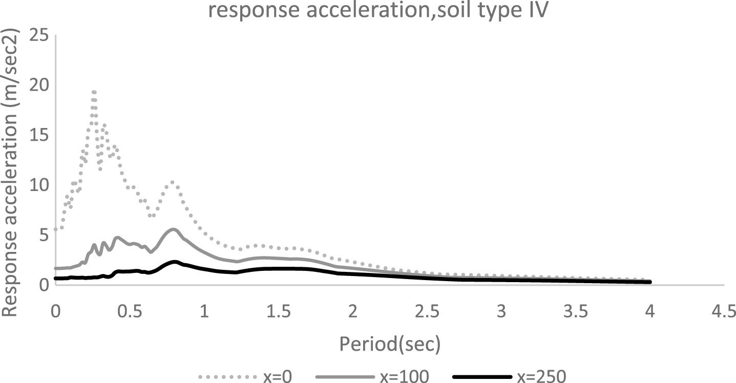
Response acceleration for soil type IV.

6.1 Effect of SVEGM on dynamic responses of the bridge

In order to investigate the effect of non-uniform ground excitations on the dynamic behavior of the bridge, uniform and non-uniform ground motions are applied on the support points of the system constructed on soil type IV. Figure 6 (a) and (b) show the relative displacement of two decks of bridge during the time.

Fig.6

(a) relative displacement of deck1 (b) relative displacement of deck2 for soil type IV.

As can be observed, displacement of two decks reduce when the effect of SVEGM is considered. It is because of both wave passage and coherency loss effects on the original ground motion along the bridge supports.

6.2 Effect of soil type on SVEGM and responses

The variation of ground motions is affected by soil types in which the waves are exciting through them. Shear wave velocity and density of each soil type are involved in ground motion excitation through the soil. In the other words, ground motion excitation in various soil types are different which affects the dynamic responses of long structures. To emphasize the importance of soil type, four types of soil classified according to the Euro code 8 are used for the base rock, firm, medium and soft soil conditions, respectively. Relative displacements of deck 2 are calculated and shown in Fig. 7 (a), (b), (c) and (d) for each soil type.

Figure 7 (a), (b), (c) and (d) show the effect of ground motion variations on the displacement of the bridge right deck (m₂). As expected, with increasing apparent wave velocity and coherency in harder soil types I and II (Fig. 7 (a) and (b)), differences between uniform and non-uniform time histories reduce and so displacement responses due to uniform and non-uniform ground motions become similar. When the bridge supports are constructed on softer soil types III and IV, differences among the ground motion time histories at the support points are more detectable. Therefore, as shown in Fig. 7(c) and (d) displacement responses of the bridge right deck are changed while considering the effect of SVEGM. Figure 7 show that uniform ground motion results in maximum displacement in comparison with non-uniform (SVEGM) excitations. Differences between uniform and non-uniform responses are about 5% to 175% in soil type I and IV respectively. It is also obvious that differences between the responses are limited to not only response amplitude but also response phase which are more apparent in soft soil.

Different displacements of two decks may lead to pounding force between the decks which occurs at almost where the relative displacement between them are more than expansion joints capacity which assumed 30 mm in this study. Figures 8 to 11 show the pounding force due to uniform and non-uniform ground motions in Fig. 4.

Fig.7

Relative displacement of deck 2 (m₂) during the SVEGM and uniform excitations for different soil types.

Fig.8

Contact force and relative displacements between decks (m₂-m₁) for soil type I.

Fig.9

Contact force and relative displacements between decks (m₂-m₁) for soil type II.

Fig.10

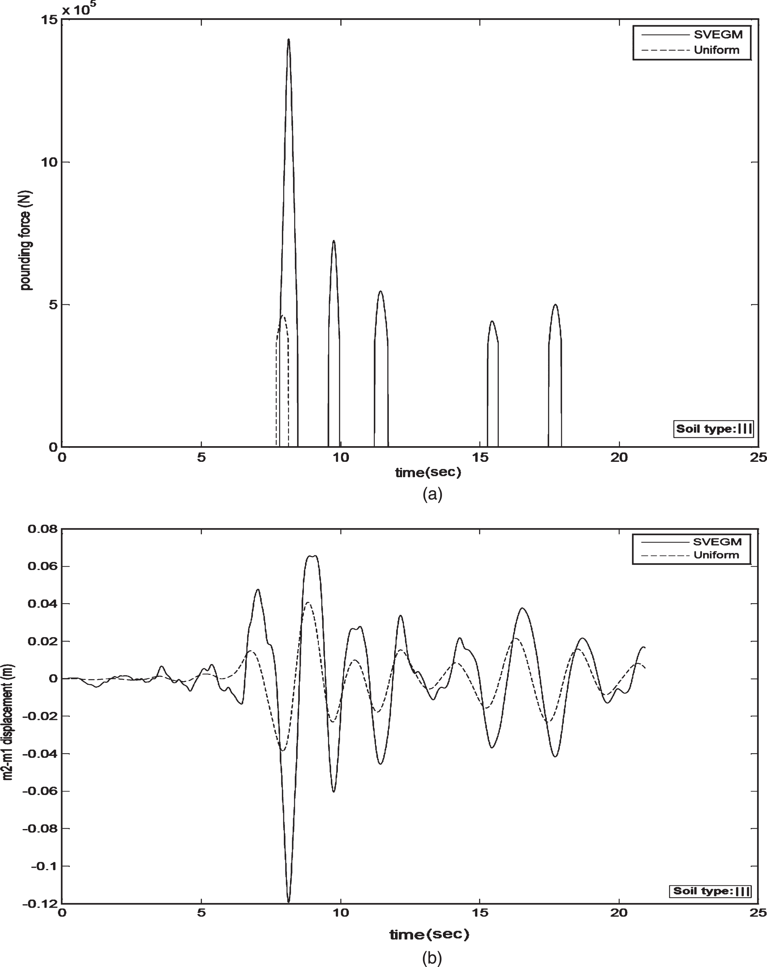
Contact force and relative displacements between decks (m₂-m₁) for soil type III.

Fig.11

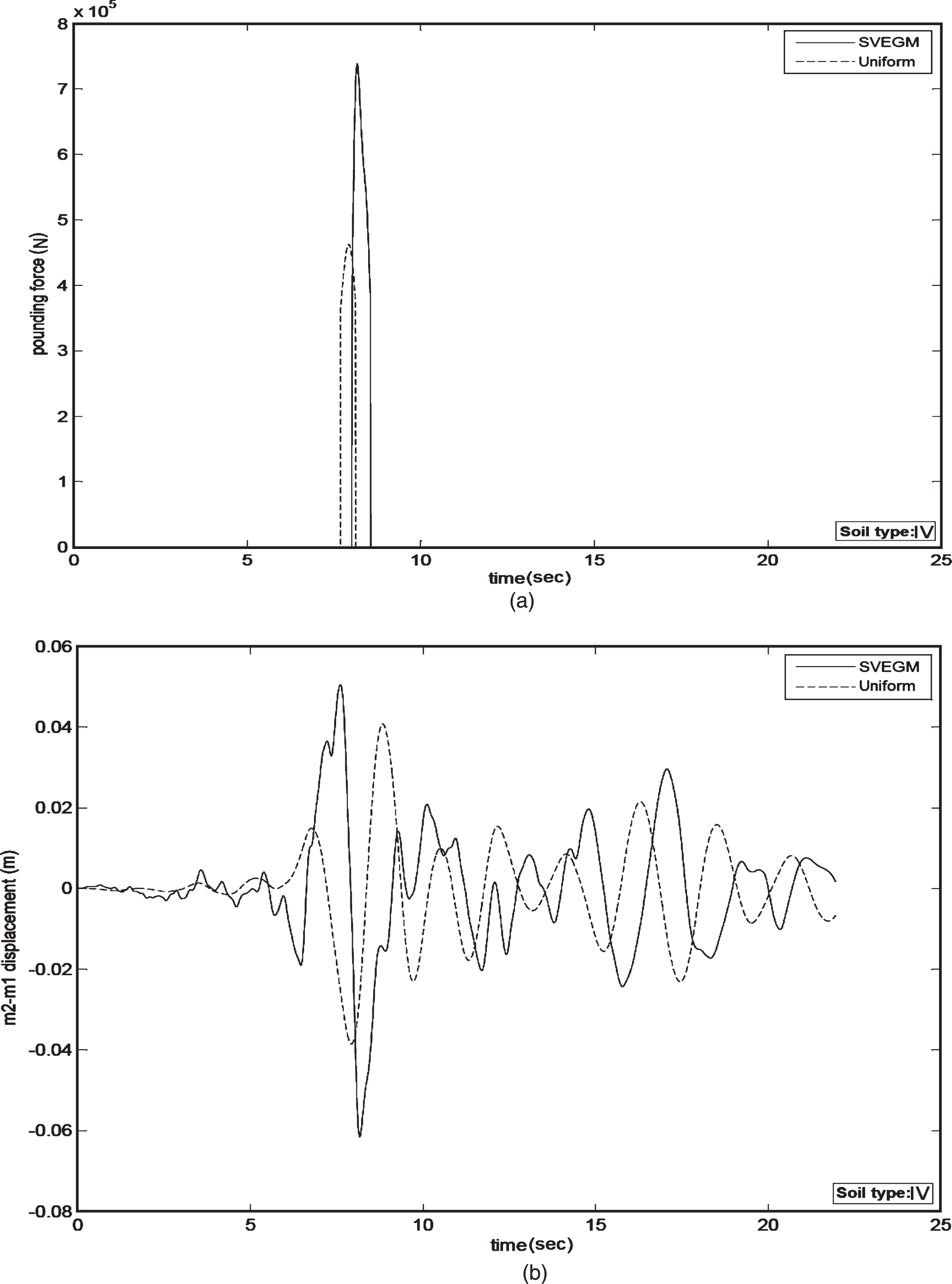
Contact force and relative displacements between decks (m₂-m₁) for soil type IV.

Figures 8 (a) to 11 (a) illustrate relative displacement between the two decks of the bridge model in the case of considering or neglecting the effect of SVEGM during the earthquake event for soil type I, II, III and IV, respectively. The relative displacement between the adjacent bridge decks determines the effect of poundings. These relative decks responses depend on the characteristics of the bridge structures, ground excitations and the support conditions of the bridge piers. In this study bridge structure characteristics and support conditions are the same. But in the case of considering the SVEGM effect, ground excitation at each support point is different from the others. Figures 8 (b) to 11 (b) show the contact force due to the ground motions in Fig. 4 for soil type I, II, III and IV, respectively. Broken lines represent the reference results due to uniform ground excitations and solid lines show the results under the effect of SVEGM in the considered gap of 30 mm. the results show that in the medium soil type III, the contact force and also the number of pounding are more than those for other soil conditions. Generally, a comparison of the results shows that the contact force due to non-uniform ground excitations is larger than that due to uniform ground motions, especially in firm and medium soil types. It should be noticed that non-uniform ground motions cause more relative displacements between two adjacent decks (m₁, m₂) and consequently larger contact force between the decks. Therefore, in all four soil types the effect of SVEGM on pounding force is not negligible. This implies that the variation of the horizontal decks displacements are under the effect of both SVEGM and soil types. This fact can be observed in contact forces between the decks. Differences between pounding forces in uniform and non-uniform cases are varied from 67% in soil type I to 187% in soil type III. The significant results show that neglecting SVEGM can cause underestimating the gap size required to prevent pounding between adjacent decks. The effect of SVEGM is not indicated in EC8 as a credible standard in the world. It seems to be needed to consider it in dynamic design of long span structures to minimize relative response, pounding potential and consequently local damage or collapse of the structures.

7 Conclusions

This paper presents the conditional method to model and simulate spatially varying earthquake ground motion time histories in which time history records along the support points of a bridge generated compatible with a known time history record and a target response spectra. For the first time a real earthquake record is used as a base record to simulate the SVEGM. A new formulation with state space analysis method is used to investigate the displacement and pounding force responses directly in time domain. A new model with ten degrees of freedom is applied for a long bridge and analyzed for the uniform and non-uniform ground motions in four types of soil. The following conclusions can be for the dynamic analysis of long bridges.

Differences between the results arise from uniform and SVEGM analysis show that considering SVEGM in seismic analysis of long bridges is necessary. The result shows that maximum displacement of the bridge decks increases about 57% in soil type III, while considering the effect of SVEGM in analysis. In building response analysis an assumption of uniform ground excitation can be justified. But in the case of bridges this assumption may not be applicable, especially when the supporting piers are far apart.

The spatial variation of the ground motions is not only determined by the characteristics of the propagating seismic waves but also by the properties of the transmitting medium. The result reveals that if the effect of SVEGM is considered in the analysis, maximum displacement of the bridge decks increases about 5%, 22%, 57% and 175% in soil type I, II, III and IV, respectively. It means moreover the effect of wave passage, soil conditions can play an important role in non-uniform generating and consequently in seismic response of the long bridges responses.

Influence of SVEGM in contact force between the adjacent decks is more significantly in firm and medium soil types. The variation of ground motions at two distant bridge support points leads to more relative displacement between the decks and contact force in comparison with the result due to uniform ground excitation. Contact force increased about 175% and 187% in soil types II and III, respectively. In general, in firm and medium local site, the larger separation distances is required to avoid pounding.

In comparison with other similar works the new formulation proposed in the current paper can be used as an appropriate method to calculate the dynamic response of a long bridge under the effect of SVEGM in time domain directly. This method calculates the bridge dynamic response more exactly because it does not need to calculate the response firstly in frequency domain and then transform it to time domain by fast Fourier transformation. Also, the proposed formulation is easier to use in comparison with numerical methods and frequency domain formulation.

Because the separation gap in conventional expansion joints are usually only a few centimeters due to serviceability consideration for smooth traffic flow, completely precluding pounding between bridge decks during strong ground motions is often not possible. The results show that contact force between two decks are significantly larger in case of considering SVEGM. The required separation distance calculate without considering non-uniform excitations may lead to underestimation of pounding force.

References

Zerva

. Response of multi-span beams to spatially incoherent seismic ground motions. Earthquake Engineering and Structural Dynamics. 1990;19:819–32.

Davoodi

, Razmkhah

, Javaheri

. Considering the effects of SVEGM on dynamic stress-strain distribution of embankment dams. Civil Engineering Infrastructures Journal. 2012;45:529–41.

Davoodi

, Jafari

, Sadreddini

. Effect of Multi-Support Excitation on Seismic Response of Embankment Dams. International Journal of Civil Engineering. 2013;11(1):19–28.

Zhao

, Wang

, Chen

, Shi

, Jiang

, Wang

. Research on the random seismic response analysis for multi-and large-span structures to multi-support excitations. Earthquake Engineering and Engineering Vibrations. 2015;14(3):527–38.

AASHTO, LRFD bridge design specifications. American Association of State Highway and Transportation Officials, Washington DC, USA; 2012.

https://nisee.berkeley.edu/elibrary/getpkg?id=SIMQKE2

Harichandran

, Wang

. Response of one- and two- span beams to spatially varying seismic excitation. Report no MSU/ENGR-88/002, Michigan (MI): Department of Civil and Environmental Engineering, College of Engineering, Michigan State University; 1988.

Perotti

. Structural response to nonstationary multiple-support random excitation. Earthquake Engineering and Structural Dynamics. 1990;19:513–27.

Zerva

. Effect of spatial variability and propagation of seismic ground motions on the response of multiply supported structures. Probabilistic Engineering Mechanics. 1991;6:212–21.

10.

Nazmy

, Abdel-Ghaffar

. Effects of ground motion spatial variability on the response of cable-stayed bridges. Earthquake Engineering and Structural Dynamics. 1992;21:1–20.

11.

Nakamura

, Der Kiureghian

, Liu

. Multiple-support response spectrum analysis of the Golden Gate Bridge. Report no. UCB/EERC-93/05, Berkeley (CA): Earthquake Engineering Research Center, College of Engineering, University of California; 1993.

12.

Harichandran

, Hawwari

, Swidden

. Response of long-span bridges to spatially varying ground motion. Journal of Structural Engineering. 1996;122(5):476–84.

13.

Der Kiureghian

, Keshishian

, Hakobian

. Multiple support response spectrum analysis of bridge including the site-response effect and MSRS code. Report no UCB/EERC-97/02, Berkeley (CA): Earthquake Engineering Research Center, College of Engineering, University of California; 1997.

14.

Soyluk

, Sicacik

. Soil-structure interaction analysis of cable-stayed bridges for spatially varying ground motion components. Soil Dynamics and Earthquake Engineering. 2012;35:80–90.

15.

, Hao

, Chouw

. Influence of ground motion spatial variation, site condition and SSI on the required separation distances of bridge structures to avoid seismic pounding. Earthquake Engineering and Structural Dynamics. 2011;40:1027–43.

16.

Apaydin

, Bas

, Harmandar

. Response of the Fatih Sultan Mehmet Suspension Bridge under spatially varying multi-point earthquake excitations. Soil Dynamics and Earthquake Engineering. 2016;84:44–54.

17.

Adanur

, Altunisik

, Soyluk

, Bayraktar

. Multiple-support seismic response of Bosporus Suspension Bridge for various random vibration method. Case Studies in Structural Engineering. 2016;5:54–67.

18.

Morris

. Dynamic analysis of cable-stiffened structures. Journal of Structural Engineering Division ASCE. 1974;100:971–81.

19.

Nazmy

, Abdel-Ghaffar

. Seismic response analysis of cable stayed bridges subjected to uniform and multiple-support excitations. Report no 87-SM-1, Princeton (NJ): Department of Civil Engineering, Princeton University; 1987.

20.

Nazmy

, Abdel-Ghaffar

. Non-linear earthquake-response analysis of long-span cable-stayed bridges: Theory. Earthquake Engineering and Structural Dynamics. 1990;19:45–62.

21.

Nazmy

, Abdel-Ghaffar

. Non-linear earthquake-response analysis of long-span cable-stayed bridges: Applications. Earthquake Engineering and Structural Dynamics. 1990;19:63–76.

22.

, Hao

. Numerical simulation of pounding damage to bridge structures under spatially varying ground motions. Engineering Structures. 2013;46:62–76.

23.

, Chouw

. Experimental investigation of inelastice response under spatially vaying excitations with pounding. Engineering Structures. 2014;79:106–16.

24.

Kaiming

, Hao

. Modelling and simulation of spatially varying earthquake ground motions at sites with varying conditions. Probabilistic Engineering Mechanics. 2012;29:92–04.

25.

Karmakar

, Ray-Chaudhuri

, Shinozuka

. Seismic response evaluation of retrofitted Vincent Thomas Bridge under spatially variable ground motions. Soil Dynamics and Earthquake Engineering. 2012;42:119–27.

26.

Wang

, Carr

, Cooke

, Moss

. The response of a 344m long bridge to non-uniform earthquake ground motions. Engineering Structures. 2009;31:2554–67.

27.

Chouw

, Hao

. Significance of SSI and nonuniform near-fault ground motions in brige response I: Effect on response with conventional expansion joint. Engineering Structures. 2008;30:141–53.

28.

Chouw

, Hao

. Significance of SSI and nonuniform near-fault ground motions in brige response II: Effect on response with modular expansion joint. Engineering Structures. 2008;30:154–62.

29.

Erhan

, Dicleli

. Effect of dynamic soil-bridge interaction modeling assumptions on the calculated seismic response of integral bridges. Soil Dynamics and Earthquake Engineering. 2014;66:42–55.

30.

Callisto

, Rampello

, Viggiani

GMB

. Soil-structure interaction for the seismic design of the Messina Strait Bridge. Soil Dynamics and Earthquake Engineering. 2013;52:103–15.

31.

Shirgir

, Ghanbari

, Shahrouzi

. Natural frequency of single pier bridges considering soil-structure interaction. Journal of Earthquake Engineering. 2016;20:611–32.

32.

Fenton

. Error evaluation of three random fields. ASCE Journal of Engineering Mechanics. 1994;120(12):2487–94.

33.

Fenton

. Simulation and analysis of random fields. Ph.D thesis, Princeton University, New Jeresy; 1990.

34.

Heredia-Zavoni

. Structural response to spatially varying earthquake ground motion. Ph.D thesis, Princeton University, New Jeresy; 1993.

35.

Eurocode 8. Design of structures for earthquake resistance. General rules, seismic actions and rules for buildings, Brussels; 2004.

36.

Chopra

. Dynamics of Structures Theory and Applications to Earthquake Engineering. Prentice Hall, Upper Saddle River, NJ; 1995.

37.

Datta

. Seismic analysis of structures. John Wiley & Sons (Asia) Pte Ltd, 2 Clementi Loop, 02-01, Singapore; 2010.

38.

Hart

, Wong

. Structural dynamics for structural engineering. John wiley and Sons; 2000.

Evaluation of long bridges dynamic responses under the effect of spatially varying earthquake ground motion

Abstract

Keywords

1 Introduction

3 Proposed model for the bridge

Table 2 Parameters of local site conditions Soil type Shear wave Damping velocity Vs(m/s) ratio ξ Base rock (I) 2000 0.05 Firm soil (II) 600 0.05 Medium soil (III) 300 0.05 Soft soil (IV) 100 0.05

References

Table 2
Parameters of local site conditions

Soil type Shear wave Damping

velocity Vs(m/s) ratio ξ

Base rock (I) 2000 0.05

Firm soil (II) 600 0.05

Medium soil (III) 300 0.05

Soft soil (IV) 100 0.05