Theoretical effects of geometrical parameters on reinforced concrete box culverts

Abstract

In this paper, a parametric study that investigated geometrical parameters of reinforced concrete box culverts (RCBC) is presented. Dead and live loads, which act on RCBC, and derivation of vehicle load formulas were explained. These formulas were verified by comparison with experimental studies. Span width, culvert height and fill depth effects on RCBC design were investigated by creating a number of 88 2D finite element culvert models. An Excel sheet was developed by using VBA and CSI API to establish SAP2000 models and to generate analysis results. Analysis results revealed that while vehicle load was predominant for fills that did not have a depth value greater than 1 m, vertical earth load was predominant beyond this value. Minimum values of internal forces and base soil pressures occurred at 0.7–1.0 m fill depth range. It is concluded that span width and fill depth parameters have an important effect on internal forces of RCBC models. This research also reveals that using multiple cell RCBC instead of using wider span width in single cell RCBC is more reliable due to much lower internal forces and base soil stresses.

Keywords

Reinforced concrete box culvert multiple cell vehicle span width fill depth

1 Introduction

Reinforced concrete box culverts (RCBC) are often used under roads for the conveyance of water and used at road-pipeline crossings to ensure safety of pipelines. A typical culvert is embedded in soil and subjected to earth and vehicle loads. RCBC can have either single cell or multiple cells and can be categorized by the construction type as cast-in-place or precast [1].

The current American Association of State Highway and Transportation Officials Standard Specifications for Highway Bridges (AASHTO SSHB) is mainly used for analysis of RCBC [2]. Although there is a great deal of experimental study that investigates effects of loads on RCBC, there are a few studies that investigate theoretical effects of geometrical parameters on RCBC. Understanding the effects of these parameters is important for achieving more economical and reliable designs.

The main objective of this study is to investigate the theoretical effects of geometrical parameters such as span width, culvert height and fill depth on RCBC design through an extensive parametric analysis. Another objective is to explain the derivation of vehicle load distribution formulas, analysis and design procedures of RCBC in detail.

1.1 Literature review

Previous studies have shown that results of experimental studies on culverts have been in a good agreement with AASHTO SSHB analysis methods. Some of essential experimental studies are referred here.

Abdel-Karim et al. [3] conducted a full-scale experiment of a double cell reinforced concrete box culvert and investigated live load distribution through soil. Experimental live load tests indicated that live load distribution in longitudinal and transverse direction is nearly same and they recommended that usage of live load distribution over a square area can be continued. They also found that after 8 ft. (2.44 m) of fill depth live load effect decreased considerably and thus AASHTO’s distinction between single and multiple RCBC is inessential for live load distribution. In the tests, AASHTO’s 1.75 vehicle load distribution factor was validated regardless of fill depth [3].

Chen et al. [4] also conducted a full-scale experiment to address the issue of vertical earth pressures not being accurately estimated. They also conducted a finite element model for comparison. The study concluded that overburden pressure calculated by the AASHTO SSHB method is accurate and in a good agreement with the test results. They also found that height of the backfill, width of the trench, slope angle of the trench, stiffness and dimensions of the culvert, and the material properties of the backfill and the foundation soil affect the vertical earth pressure on the culvert [4].

Pimentel et al. [5] conducted an experiment of a reinforced concrete box culvert with 9.5 m embankment depth. A nonlinear finite element model was also used to investigate nonlinear and elastic behaviour of concrete box culvert. After finding experimental results and finite element analysis results were close, a parametric study was done to evaluate soil-structure interaction and failure mechanism of concrete box culverts. Soil interaction analysis results showed that soil-interaction factor varies between AASHTO compacted side fill and uncompacted side fill interaction factors. This study also indicated that overburden pressure caused by fill depth is greater than the normal weight of embankment above the culvert [5].

Wood et al. [6] performed analyses of two production-oriented culvert load-rating demand models by using live-load test data from three instrumented RCBC under four different soil depths. A two-dimensional (2D) structural-frame model (named as Level 1) with simple supports and uniform reaction loads as base soil and a 2D soil-structure interaction model (named as Level 3) were used as demand models. Increasing model sophistication generated higher precision and accuracy for predicted moments, as expected. However, Level 1 model had high precision and accuracy for predicting moment values at the top exterior wall corners and the top midspans of culverts, too. Predicted moment demands for bottom slabs and corners were conservative in both model groups. However, increasing model sophistication of Level 1 group by adding linear springs as base soil could improve precision and accuracy for predicted moments at bottom slabs and corners [6].

Orton et al. [7] conducted a full-scale experiment of 10 existing reinforced concrete box culverts and investigated the effects of live load (truck loads) on reinforced concrete box culverts. Fill depths of the culverts were ranging from 0.78 m to 4.04 m and span widths were greater than 6 m (20 ft.). They used 12 reusable strain transducers and 12 linear variable displacement transducers to measure strain and displacement values. Experimental live load tests indicated that the live-load effect decreased significantly with increasing fill depth. They also found that the 2012 AASHTO LRFD bridge design specifications predicted strains and displacements overly conservative when compared with the field data for fill depths less than 2.4 m (8 ft) [7].

2 Culvert models and parameters

2.1 Material properties

The embankment used for the sides and above culverts was assumed to have γ= 18 kN/m³ unit weight and Φ= 30° friction angle. To model base soil, springs with 30×10³ kN/m³ stiffness constant were used. The concrete used to model the culverts had 25 MPa characteristic compressive strength, 30 GPa modulus of elasticity and 0.2 Poisson’s ratio.

2.2 Geometry

A typical reinforced concrete box culvert model and geometric symbols used in this study are shown in Fig. 2. Z is fill depth above the culvert, which is measured between the outer face of top slab and top of the fill. S is effective span width of the culvert, which is measured between centers of exterior walls. B_C is top slab width of box culvert, which is measured between the outside faces of exterior walls. H_C is effective height of the culvert, which is measured between centers of top and bottom slabs. t is section thickness of the culvert elements. Section thickness (t) for culverts is assumed to have minimum value of 15 cm and calculated as one twenty of span width (15 cm ≤ S/20). Section thickness for each model is constant for slabs and walls. Design length (L) of culvert models was kept constant as 1 m for all models.

Fig.1

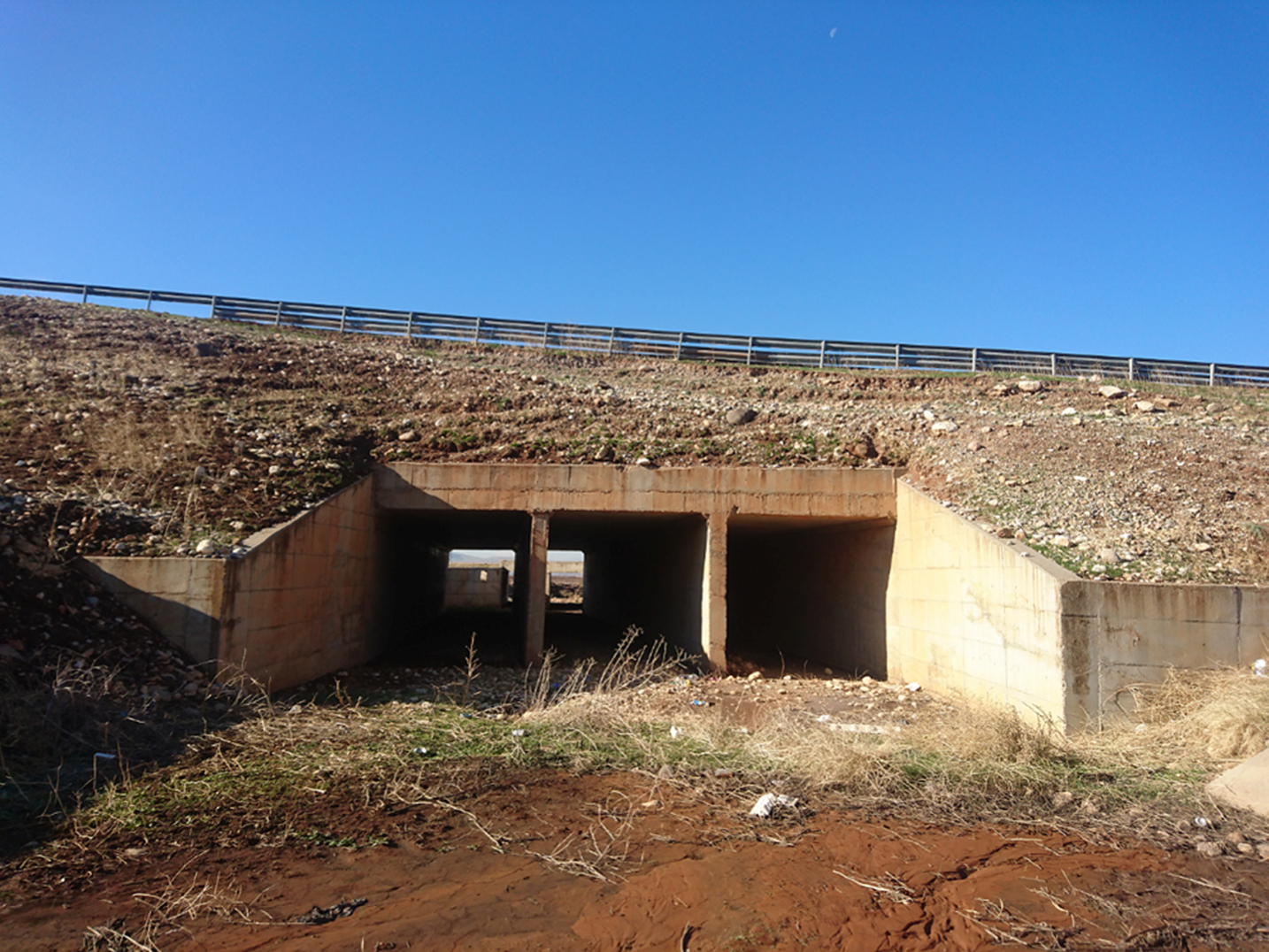
Picture of a typical reinforced concrete box culvert (image by Mesut Kuş).

Fig.2

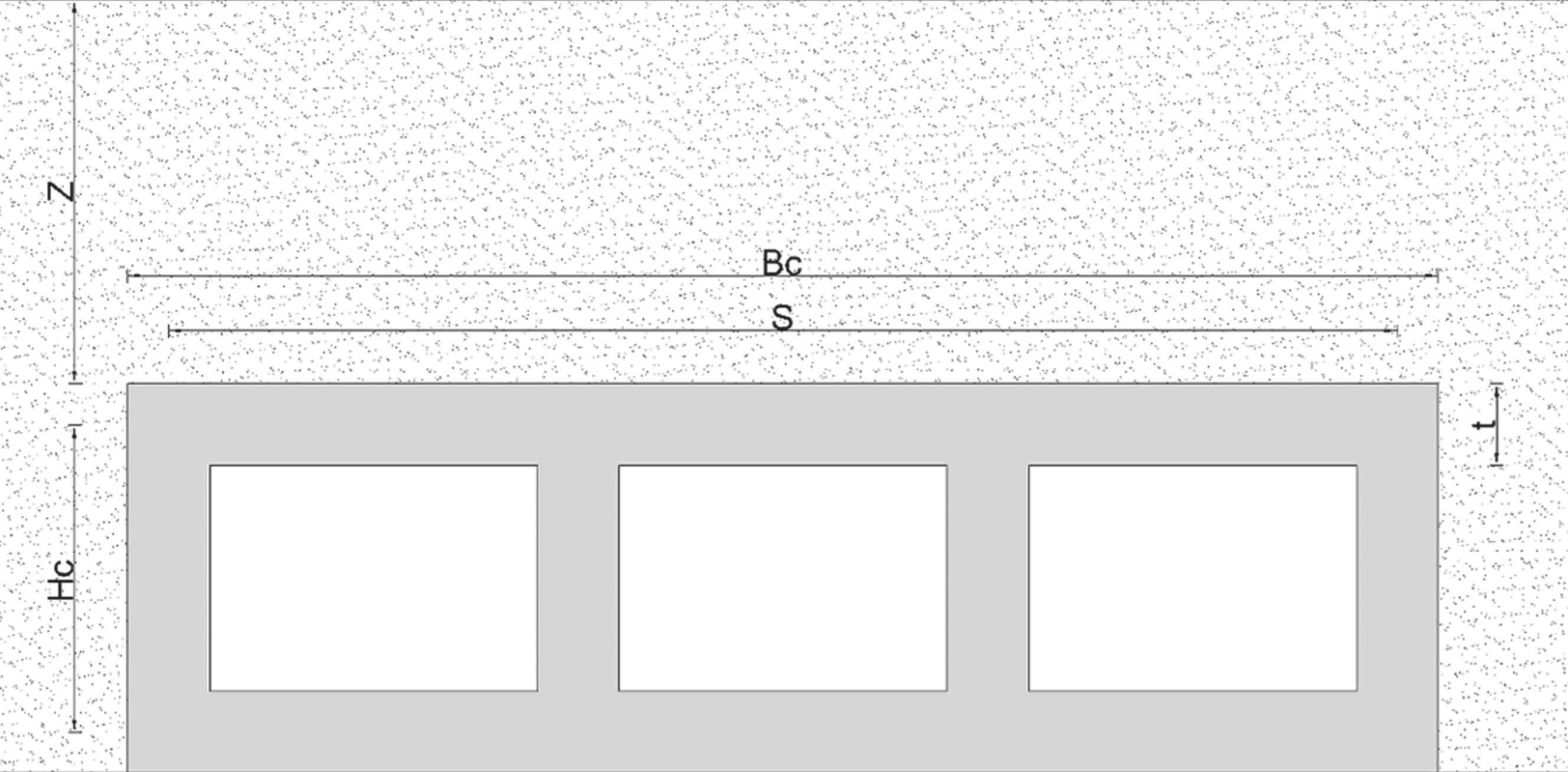
Typical reinforced concrete box culvert model and symbols.

As shown in Table 1, three model groups and 88 models were used for the analysis. In the first group, one cell concrete box culverts were considered. First model group consisted of four cases, which were categorized according to the fill depth. 0.50 m, 0.70 m, 1.50 m, and 3 m of fill depths were considered for Case I, Case II, Case III and Case IV, respectively. 2.40 m of constant culvert height was used for first group. Span width was changed between 0.60 m and 9.60 m.

Table 1

Parameters of reinforced concrete box culvert models

Group	Case	No	Z	S	Hc	t	Cell	Group	Case	No	Z	S	Hc	t	Cell
			m	m	m	m	Number				m	m	m	m	Number
1. Group	WIDTH	1	0.50	0.60	2.40	0.15	1	2. Group	HEIGHT	45	0.70	1.00	2.50	0.15	1
	CASE I	2	0.50	1.20	2.40	0.15	1		CASE II	46	0.70	1.00	3.00	0.15	1
	Z = 0.5 m	3	0.50	2.00	2.40	0.15	1		Z = 0.7 m	47	0.70	1.00	3.50	0.15	1
		4	0.50	3.00	2.40	0.15	1			48	0.70	1.00	4.00	0.15	1
		5	0.50	4.00	2.40	0.20	1		HEIGHT	49	1.50	1.00	0.60	0.15	1
		6	0.50	5.00	2.40	0.25	1		CASE III	50	1.50	1.00	1.00	0.15	1
		7	0.50	7.00	2.40	0.35	1		Z = 1.5 m	51	1.50	1.00	1.50	0.15	1
		8	0.50	9.60	2.40	0.48	1			52	1.50	1.00	2.00	0.15	1
	WIDTH	9	0.70	0.60	2.40	0.15	1			53	1.50	1.00	2.50	0.15	1
	CASE II	10	0.70	1.20	2.40	0.15	1			54	1.50	1.00	3.00	0.15	1
	Z = 0.7 m	11	0.70	2.00	2.40	0.15	1			55	1.50	1.00	3.50	0.15	1
		12	0.70	3.00	2.40	0.15	1			56	1.50	1.00	4.00	0.15	1
		13	0.70	4.00	2.40	0.20	1		HEIGHT	57	3.00	1.00	0.60	0.15	1
		14	0.70	5.00	2.40	0.25	1		CASE	58	3.00	1.00	1.00	0.15	1
		15	0.70	7.00	2.40	0.35	1		IV Z = 3.0 m	59	3.00	1.00	1.50	0.15	1
		16	0.70	9.60	2.40	0.48	1			60	3.00	1.00	2.00	0.15	1
	WIDTH	17	1.50	0.60	2.40	0.15	1			61	3.00	1.00	2.50	0.15	1
	CASE III	18	1.50	1.20	2.40	0.15	1			62	3.00	1.00	3.00	0.15	1
	Z = 1.5 m	19	1.50	2.00	2.40	0.15	1			63	3.00	1.00	3.50	0.15	1
		20	1.50	3.00	2.40	0.15	1			64	3.00	1.00	4.00	0.15	1
		21	1.50	4.00	2.40	0.20	1	3. Group	ONE	65	0.00	9.60	2.40	0.48	1
		22	1.50	5.00	2.40	0.25	1		CELL Z	66	0.50	9.60	2.40	0.48	1
		23	1.50	7.00	2.40	0.35	1		is 0 to 5 m	67	0.70	9.60	2.40	0.48	1
		24	1.50	9.60	2.40	0.48	1			68	1.00	9.60	2.40	0.48	1
	WIDTH	25	3.00	0.60	2.40	0.15	1			69	2.00	9.60	2.40	0.48	1
	CASE IV	26	3.00	1.20	2.40	0.15	1			70	3.00	9.60	2.40	0.48	1
	Z = 3.0 m	27	3.00	2.00	2.40	0.15	1			71	4.00	9.60	2.40	0.48	1
		28	3.00	3.00	2.40	0.15	1			72	5.00	9.60	2.40	0.48	1
		29	3.00	4.00	2.40	0.20	1		DOUBLE	73	0.00	9.60	2.40	0.48	2
		30	3.00	5.00	2.40	0.25	1		CELL Z	74	0.50	9.60	2.40	0.48	2
		31	3.00	7.00	2.40	0.35	1		is 0 to 5 m	75	0.70	9.60	2.40	0.48	2
		32	3.00	9.60	2.40	0.48	1			76	1.00	9.60	2.40	0.48	2
2. Group	HEIGHT	33	0.50	1.00	0.60	0.15	1			77	2.00	9.60	2.40	0.48	2
	CASE I	34	0.50	1.00	1.00	0.15	1			78	3.00	9.60	2.40	0.48	2
	Z = 0.5 m	35	0.50	1.00	1.50	0.15	1			79	4.00	9.60	2.40	0.48	2
		36	0.50	1.00	2.00	0.15	1			80	5.00	9.60	2.40	0.48	2
		37	0.50	1.00	2.50	0.15	1		TRIPPLE	81	0.00	9.60	2.40	0.48	3
		38	0.50	1.00	3.00	0.15	1		CELL Z	82	0.50	9.60	2.40	0.48	3
		39	0.50	1.00	3.50	0.15	1		is 0 to 5 m	83	0.70	9.60	2.40	0.48	3
		40	0.50	1.00	4.00	0.15	1			84	1.00	9.60	2.40	0.48	3
	HEIGHT	41	0.70	1.00	0.60	0.15	1			85	2.00	9.60	2.40	0.48	3
	CASE II	42	0.70	1.00	1.00	0.15	1			86	3.00	9.60	2.40	0.48	3
	Z = 0.7 m	43	0.70	1.00	1.50	0.15	1			87	4.00	9.60	2.40	0.48	3
		44	0.70	1.00	2.00	0.15	1			88	5.00	9.60	2.40	0.48	3

The second group was similar to the first group; however, in this group, culvert height was changed between 0.60 m and 4.00 m with a constant 1 m span width and a constant 15 cm section thickness.

In the third group, multiple numbered culvert cells were considered. 9.60 m constant span width and 2.40 m constant culvert height were used. Since the span width was constant, section thickness was constant too, and calculated as 48 cm (960/20). The one cell culvert with these dimensions was considered as Case I for the third group and this culvert was divided into double cells and triple cells, which were named as Case II and Case III, respectively. For the third group, fill depth was changed between 0 m and 5 m.

3 Loading

Figure 3 shows the static model and load types considered for concrete box culverts. Dead loads consist of vertical and lateral earth pressures and self weight of the culvert. AASHTO HS20 vehicle load and lateral surcharge load were applied as live load. Base soil was modeled by using linear springs.

Fig.3

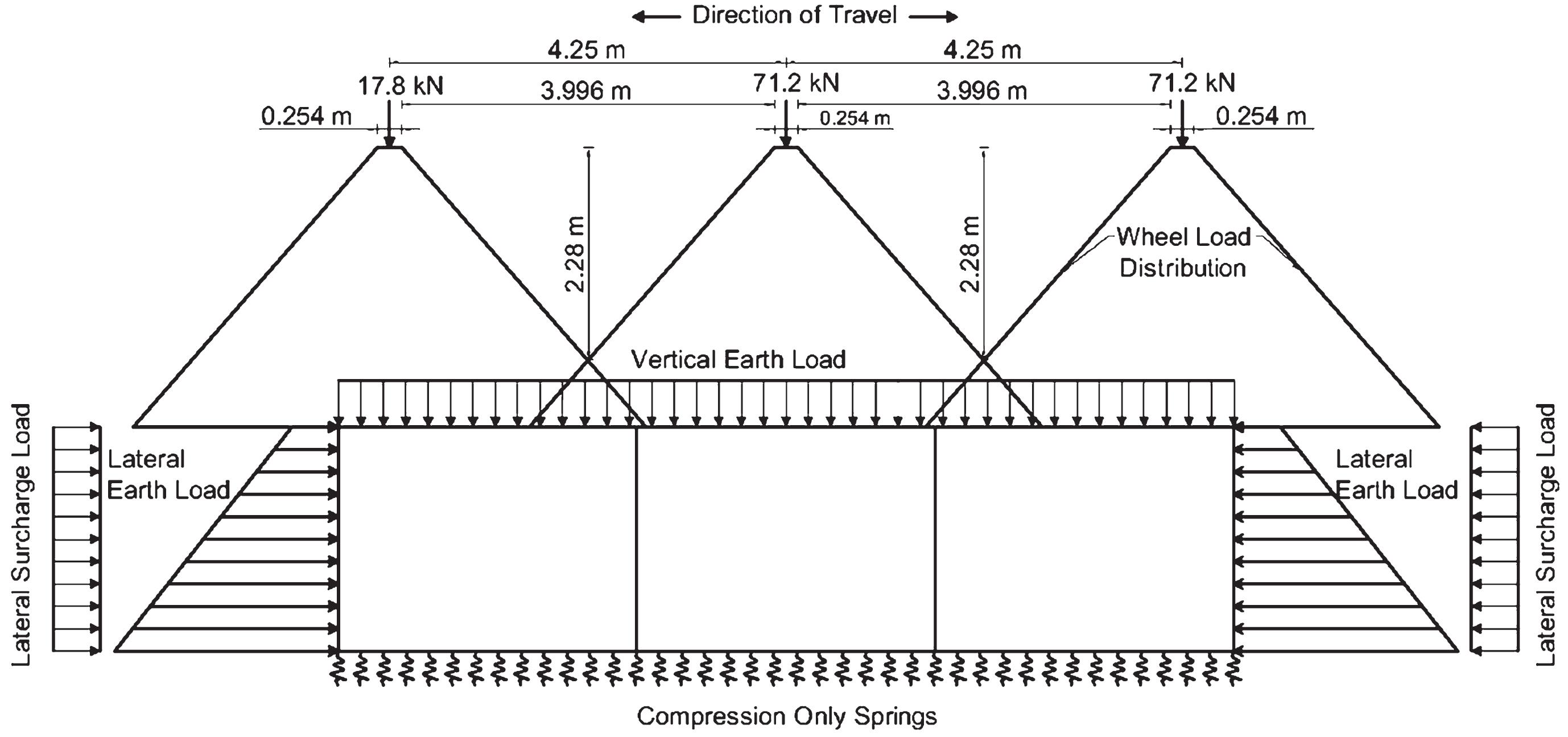
Static model and loads for concrete box culverts.

3.1 Dead loads

3.1.1 Vertical earth pressure

The fill depth above culverts is an important factor that affects the design of reinforced box culverts since it affects both fill weight and distribution of vehicle loads. Previous studies have shown that overburden pressure caused by fill depth is greater than the normal weight of embankment above the culvert [4, 5]. Therefore, the AASHTO SSHB uses different soil-interaction factors according to the embankment installation type as stated in Articles 16.6.4.2.1 and 16.6.4.2.2 [2]. In this study, embankment installation type with compacted side fills was considered. $F_{e} = 1 + 0.20 \frac{Z}{B_{C}} \leq 1.15$ (1) where F_e is soil-interaction factor, Z is fill depth and B_C is top slab width of box culvert.

As stated in the AASHTO SSHB Article 16.6.4.2, the total overburden pressure W_E on the box culvert is calculated as: [2] $W_{E} = F_{e} γ B_{C} Z (kN / m)$ (2) where γ is unit weight of soil used for embankment. This equation is converted to uniformly distributed vertical earth load dividing by B_C: $DL = F_{e} γ Z ({kN / m}^{2})$ (3)

Vertical earth load was applied to the top slab of culvert as uniformly distributed load as shown in Fig. 3.

3.1.2 Lateral earth pressure

Soil at the sides of box culvert was considered at rest condition. The following equation was used to calculate at rest earth coefficient: [8] $K_{0} = 1 - \sin (Φ)$ (4)

Since friction angle was taken Φ= 30° in the culvert models, K₀ was calculated as 0.5 by using Equation 4. As shown in Fig. 3, lateral earth load was modeled as trapezoidal load, which starts from the center of top slab and finishes at the center of bottom slab. Lateral earth pressure at the start point EP₁ and lateral earth pressure at the end point EP₂ were calculated by using the following equations for 1 m design length: ${EP}_{1} = K_{0} γ (Z + \frac{t}{2}) ({kN / m}^{2})$ (5) ${EP}_{2} = K_{0} γ (Z + \frac{t}{2} + H_{C}) ({kN / m}^{2})$ (6)

3.1.3 Self weight

The self weight of concrete box culvert was also considered in the analyses. Concrete members were modeled with 25 kN/m³ unit weight.

3.2 Live loads

3.2.1 Vehicle load

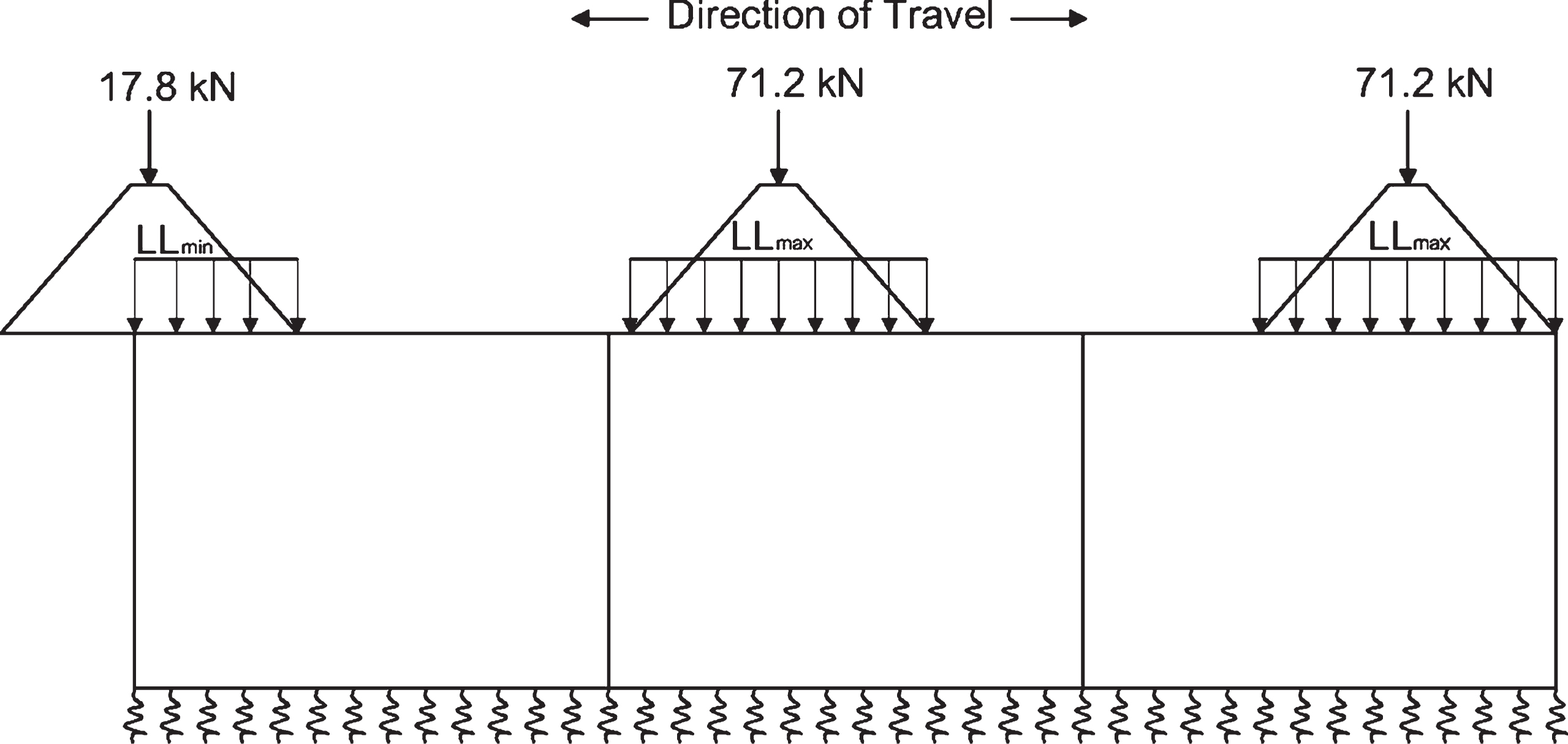
AASHTO HS20 vehicle loading was considered at this study. AASHTO HS20 truck has two different sizes of wheels. These are single wheel with 0.254 m×0.254 m (10 inches×10 inches) dimensions and dual wheel with 0.254 m×0.508 m (10 inches×20 inches) dimensions as shown in Fig. 4 [9]. Front wheels have 17.8 kN load while middle and rear wheels have 71.2 kN load as shown in Fig. 3. These wheel loads are applied as uniformly distributed load and moved all together along the span until wheel load projection of the first wheel leaves the span.

Fig.4

Spacing and dimensions for HS20 truck wheels and axles [9].

There are two main equations for the distribution width of wheel loads. The first one is stated in AASHTO SSHB Article 16.7.4.1 and 3.24.3.2. When the fill cover is equal or less than 0.6 m (2 ft.), wheel loads shall be distributed over a distribution width calculated by the following equation: [2] $E_{1} = 1.2 + 0.06 S \leq 2.13 m$ (7) where E₁ is distribution width for the first distribution case and S is effective span width. E₁ shall not exceed 2.13 m (7 ft.). Uniformly distributed vehicle loads for this distribution case can be written as for 1 m design length: ${LL}_{\max 1} = \frac{P_{\max}}{E_{1}} ({kN / m}^{2})$ (8) ${LL}_{\min 1} = \frac{P_{\min}}{E_{1}} ({kN / m}^{2})$ (9) where P_max is maximum wheel load, which is 71.2 kN for HS20 truck, P_min is minimum wheel load, which is 17.8 kN for HS20 truck. LL_max and LL_min are uniformly distributed vehicle loads for maximum and minimum wheel loads, respectively.

The second main distribution width equation is for embankments, which have depth greater than 0.6 m. ASTM C890-13 in Article 5.2.3.1 states that when embankment separates the truck wheels and top surface of the culvert, wheel loads shall be distributed over a rectangle area as shown in the following equation: [9] $A = (0.254 + 1.75 Z) \times (0.508 + 1.75 Z) (m^{2})$ (10) where A is wheel load area. According to ASTM C890-13 Article 5.2.3.3, when projection areas of wheel loads intersect, the sum of wheel loads will be uniformly distributed over a combined area, which consists of exterior boundaries of the individual load areas. If load area exceeds area of top surface of concrete box culvert, only surface of the top slab shall be used for load area [9].

To formulate distribution areas, situations where load area intersections occur must be defined first. Since wheel spacing is less than axle spacing, the first intersection occurs between two wheels that are at the same axle as shown in Fig. 5. First critical fill depth can be calculated as 0.74 m from the following geometric calculation knowing that the total slope of load projection lines is 1.75.

Fig.5

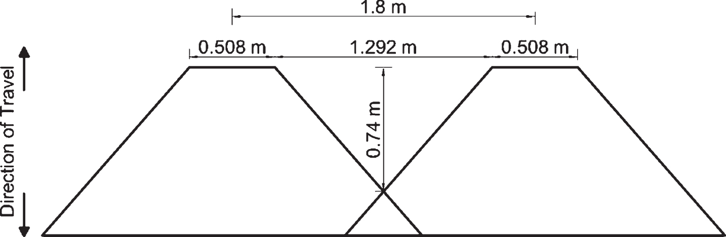
Wheel spacing and load projection for HS20 truck.

$Z_{cr 1} = \frac{1.8 - 0.508}{1.75} = \frac{1.292}{1.75} = 0.74 m$ (11)

The second intersection occurs between two axles as shown in Fig. 3. Calculation of the second critical fill depth ends up 2.28 m with the same method: $Z_{cr 2} = \frac{4.25 - 0.254}{1.75} = \frac{3.996}{1.75} = 2.28 m$ (12)

After defining critical fill depths for load projections, distribution areas can be defined. The second distribution case is valid for 0.6 m <Z <0.74 m. In this interval of fill depth, no intersection occurs between wheel load projections yet. The second distribution width and length are shown in the following equations: $E_{2} = 0.254 + 1.75 Z (m)$ (13) $L_{D 2} = 0.508 + 1.75 Z (m)$ (14) where E₂ is second distribution width and L_D2 is distribution length of dual wheels. Distribution length of single wheels L_S2 equals to E₂ for this distribution case. Distribution area for dual wheels can be obtained by multiplying E₂ and L_D2. With the same way, distribution area for single wheels is obtained as square of E₂. Uniformly distributed vehicle loads are shown in the following equations: ${LL}_{\max 2} = \frac{P_{\max}}{E_{2} L_{D 2}} ({kN / m}^{2})$ (15) ${LL}_{\min 2} = \frac{P_{\min}}{E_{2}^{2}} ({kN / m}^{2})$ (16)

The third distribution case is defined for 0.74 m ≤ Z ≤ 2.28 m. In this interval of fill depth, while intersection occurs between wheels, intersection of different axles has not occurred yet. Thus, distribution width is not changed for this case. Since load projections of two wheels at the same axle overlap, distribution lengths for this case include wheel spacing (1.8 m) and wheel lengths. For the same reason two wheel loads are included in uniformly distributed vehicle load equations. Third distribution width and lengths are shown in the following equations: $E_{3} = 0.254 + 1.75 Z (m)$ (17) $L_{S 3} = 0.254 + 1.75 Z + 1.8 (m)$ (18) $L_{D 3} = 0.508 + 1.75 Z + 1.8 (m)$ (19)

Uniformly distributed vehicle loads for the third case are shown in the following equations: ${LL}_{\max 3} = \frac{2 P_{\max}}{E_{3} L_{D 3}} ({kN / m}^{2})$ (20) ${LL}_{\min 3} = \frac{2 P_{\min}}{E_{3} L_{S 3}} ({kN / m}^{2})$ (21)

The forth distribution case is defined for 2.28 m <Z and divided in four sub cases. Since fill depth is greater than the second critical fill depth, all wheel load projection areas overlap. Span width of concrete box culvert is an important factor for this case to determine count of axles, which are in vertical projection of the span. Axles that are not in vertical projection of the span width are not considered for loading. For practicality, dual wheel length was considered when calculating distribution length in forth case and its sub cases as expressed in the following equation: $L_{4} = 0.508 + 1.75 Z + 1.8 (m)$ (22)

If effective span width S is less than or equal to axle spacing (S ≤ 4.25 m), only one axle and two wheels at this axle are considered for loading. This case is a sub case and named as 4A. Since only one axle is considered, maximum wheel load is used for uniformly distributed vehicle load. As stated in the ASTM C890-13 Article 5.2.3.4, only portion of distributed vehicle load in range of span is considered for loading by reason of distributed load area exceeds top surface of culvert in this sub case [9]. Therefore, distribution width equation is used for only calculation of distributed load value for this sub case and vehicle load is distributed over whole span width knowing that span width is smaller than distribution width. Distribution width and uniformly distributed vehicle load are defined in the following equations for sub case 4A: $E_{4 A} = 0.254 + 1.75 Z (m)$ (23) ${LL}_{4 A} = \frac{2 P_{\max}}{E_{4 A} L_{4}} ({kN / m}^{2})$ (24)

When effective span width S is less than or equal to two axle spacing and greater than one axle spacing (4.25 m <S ≤ 8.5 m), two axles and four wheels at these axles are considered for loading. This sub case is named as 4B. Since front axle has not been considered yet, maximum wheel load is used for uniformly distributed vehicle load. Distribution width for this sub case contains axle spacing (4.25 m) due to inclusion of two axles. Vehicle load is distributed over whole span width in this sub case for the same reason as explained in sub case 4A. Distribution width and uniformly distributed vehicle load for sub case 4B are defined in the following equations: $E_{4 B} = 0.254 + 1.75 Z + 4.25 (m)$ (25) ${LL}_{4 B} = \frac{4 P_{\max}}{E_{4 B} L_{4}} ({kN / m}^{2})$ (26)

When effective span width S is greater than two axle spacing (8.5 m <S), three axles and six wheels at these axles are considered for loading. This case is named as 4C. Four maximum and two minimum wheel loads are used for uniformly distributed vehicle load. Distribution width for this sub case contains two axle spacing (8.5 m) due to inclusion of three axles. Distributed vehicle loads are much smaller in forth case as shown in Fig. 6. For this reason and practicality, although effective span width can be greater than calculated distribution width, vehicle load is distributed over whole span width in this sub case, too. Distribution width and uniformly distributed vehicle load for sub case 4C are defined in the following equations:

Fig.6

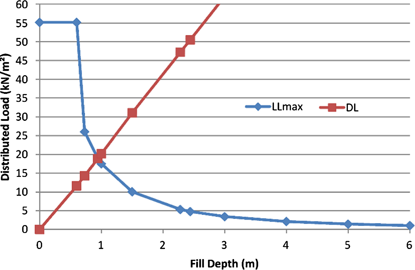
Vertical earth load and maximum distributed vehicle load variation for span width of 1.5 m.

$E_{4 C} = 0.254 + 1.75 Z + 8.5 (m)$ (27) ${LL}_{4 C} = \frac{(4 P_{\max} + 2 P_{\min})}{E_{4 C} L_{4}} ({kN / m}^{2})$ (28)

Distribution areas and distritubed vehicle load formulas for all cases are summarized in Table 2.

Table 2

Distribution width, length and distributed vehicle load formulas

Case Name	Fill Depth Interval	Span Width Interval	E m	L_S m	L_D m	LL_max kN/m²	LL_min kN/m²
1	Z ≤ 0.6 m		1.2+0.006 S ≤ 2.13 m			$\frac{P_{\max}}{E_{1}}$	$\frac{P_{\min}}{E_{1}}$
2	0.6 m <Z <0.74 m		0.254+1.75Z	0.254+1.75Z	0.508+1.75Z	$\frac{P_{\max}}{E_{2} L_{D 2}}$	$\frac{P_{\min}}{E_{2}^{2}}$
3	0.74 m ≤ Z ≤ 2.28 m		0.254+1.75Z	0.254+1.75Z+1.8	0.508+1.75Z+1.8	$\frac{2 P_{\max}}{E_{3} L_{D 3}}$	$\frac{2 P_{\min}}{E_{3} L_{S 3}}$
4A	2.28 m <Z	S ≤ 4.25 m	0.254+1.75Z	0.508+1.75Z+1.8		$\frac{2 P_{\max}}{E_{4 A} L_{4}}$
4B	2.28 m <Z	4.25 m <S ≤ 8.5 m	0.254+1.75Z+4.25	0.508+1.75Z+1.8		$\frac{4 P_{\max}}{E_{4 B} L_{4}}$
4C	2.28 m <Z	8.5 m <S	0.254+1.75Z+8.5	0.508+1.75Z+1.8		$\frac{(4 P_{\max} + 2 P_{\min})}{E_{4 C} L_{4}}$

After determination of distribution areas and distributed vehicle loads, an example graph of maximum uniformly distributed vehicle load variation with respect to fill depth was drawn in Fig. 6. As it can be seen in Fig. 6, vehicle load was at its maximum value and constant for the first case. After the first case, vehicle load was decreasing dramatically. Vertical earth load and vehicle load had the same value at fill depth of about 1 m. According to AASHTO SSHB Article 6.4.2, the effect of vehicle load can be ignored over 2.44 m (8 ft.) fill depth [2]. At this depth of fill, LL_max had a value of 4.79 kN/m² while DL had a value of 50.51 kN/m² as shown in Fig. 6. In other words, distributed vehicle load was 9.48 percent of distributed overburden load at 2.44 m fill depth. In this study vehicle load was not neglected at any depth of fill value.

3.2.2 Verification of distributed vehicle load formulas

Vehicle load formulas compared with two experimental studies for verification. In the first study, Abdel-Karim et al. [3] placed pressure sensors on top of a double cell reinforced concrete box culvert with 3.66 m×3.66 m cell dimensions. A test truck which had two axles and had 50.71 kN rear, 9.34 kN front wheel loads was used for the tests. The axles were spaced approximately 4.25 m on center. The culvert was covered with different height of fills. A zero reading was performed at each fill level to indicate vertical earth pressure, and then the testing truck crossed the culvert. They measured vehicle and soil fill load separately by this way [3].

To use these test data for verification, span width of the culvert was needed. Since researchers didn’t give slab width or wall thickness values of the culvert in the study, the culvert was assumed to have 0.18 m (3.66/20) wall thickness and 7.86 m (2*3.66+3*0.18) span width. The test truck wasn’t an AASHTO HS20 truck. Since it was shorter and missing one rear axle, Equation 26 was modified as (2*P_max+2*P_min)/(E_4B*L₄). Test results of the study and calculated vehicle load values by using Table 2 formulas are shown in Table 3 and Fig. 7. Both unmodified and modified calculations are given, and they are named as LLmax-HS20 and LLmax-Test Truck, respectively.

Table 3
Vehicle load results based on field data and calculated values

Fill Depth (Z) E Ls L LLmax-HS20 LLmax-Test Truck LLmax-Abdel-Karim

m m m m kN/m² kN/m² kN/m²

0.61 1.322 1.322 1.576 24.34 24.34 14.36

1.07 2.127 3.927 4.181 11.40 11.40 16.28

1.83 3.457 5.257 5.511 5.32 5.32 10.05

2.44 8.774 6.578 6.578 3.51 2.08 4.79

3.05 9.842 7.646 7.646 2.70 1.60 2.87

3.66 10.909 8.713 8.713 2.13 1.26 1.34

Fill Depth (Z)	E	Ls	L	LLmax-HS20	LLmax-Test Truck	LLmax-Abdel-Karim
0.61	1.322	1.322	1.576	24.34	24.34	14.36
1.07	2.127	3.927	4.181	11.40	11.40	16.28
1.83	3.457	5.257	5.511	5.32	5.32	10.05
2.44	8.774	6.578	6.578	3.51	2.08	4.79
3.05	9.842	7.646	7.646	2.70	1.60	2.87
3.66	10.909	8.713	8.713	2.13	1.26	1.34

Fig.7

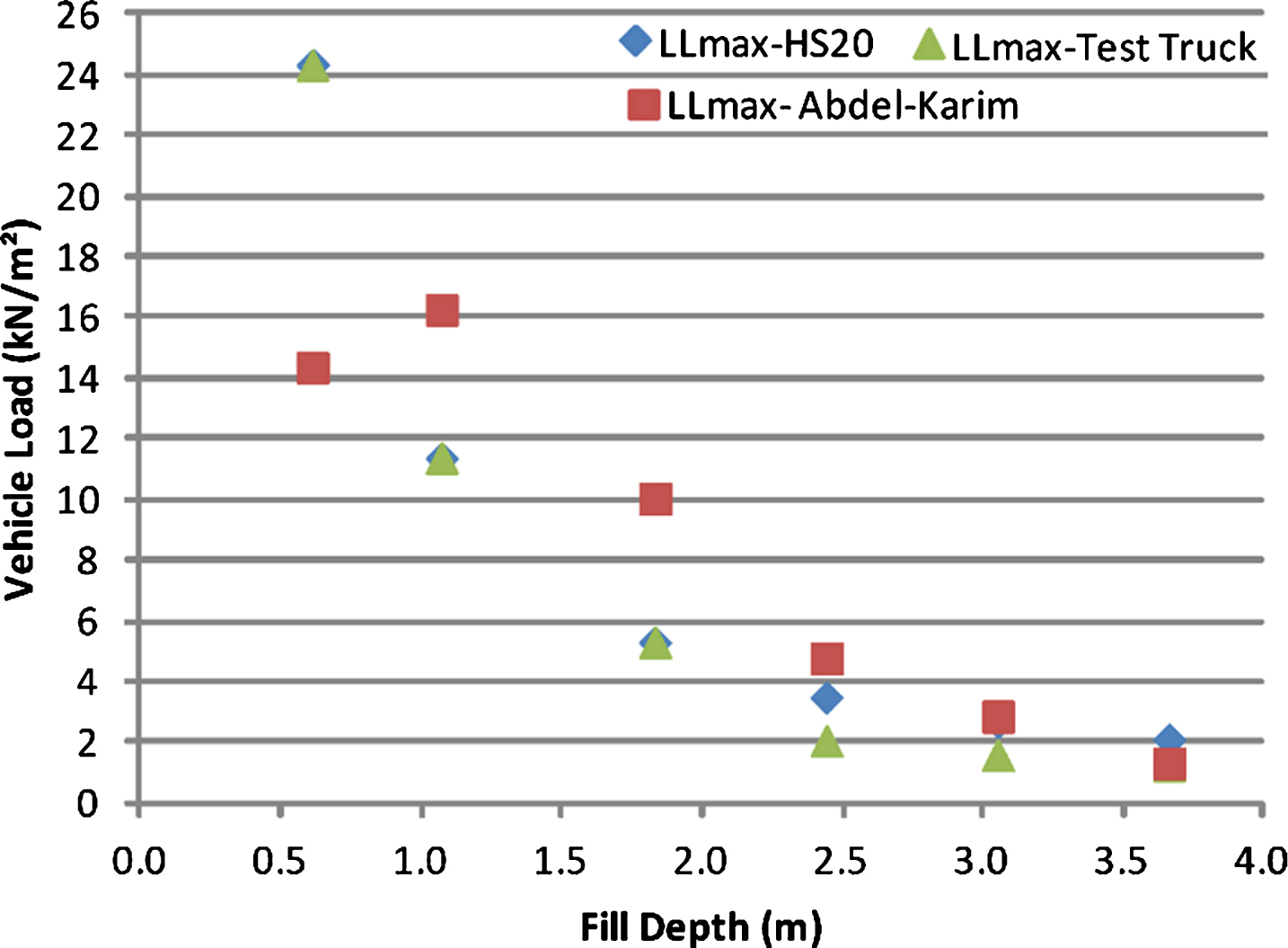
Comparison of vehicle load based on field data and calculated values.

There was a sharp decline in vehicle loads as fill depth was increased except for 0.61 m (2 ft.) fill depth as Abdel-Karim et al. [3] pointed out. In their opinion, this reduction in vehicle load reading was due to a misplacing of rear axles according to measurement instrument. The calculated vehicle loads were generally smaller than the test results. It is important to note that test results represent peak vehicle load values occurred over top slab, in spite of that calculated vehicle loads represent a single uniformly distributed load value for each fill depth level. Therefore, this difference between peak test load values and calculated load values can be expected.

In the second study, Orton et al. [7] placed 12 reusable strain transducers and 12 linear variable displacement transducers under top slabs of 10 existing reinforced concrete box culverts. They compared test results with RS3 software, The AASHTO (2002) Load Factor Design (LFD) and The 2012 AASHTO LRFD bridge design specifications. A test truck which had two rear axles and one front axle and had approximately 40 kN rear wheel loads was used for the tests. The rear axles were spaced 1.20 m on center [7]. Detailed data and results for the study were taken from report which Orton et al. [10] prepared for Missouri Department of Transportation [10].

The test truck wasn’t an AASHTO HS20 truck in this study, too. The front axle was assumed to be located approximately 4.25 m ahead the nearest rear axle. The distance of the farthest axles of the truck was assumed to be 5.45 m (1.2+4.25). Therefore, 0.254+1.75*Z+1.2 equation was used as distribution width and (4*P_max)/(E*L) was used as wheel load equation when the fill depth values were below the 2.28 m or span width not exceeding 5.45 m. After the 2.28 m fill depth and when the span width values were exceeding 5.45 m, 0.254+1.75*Z+5.45 equation was used as distribution width and (4*P_max+2*P_min)/(E*L) was used as wheel load equation. Although researchers didn’t use front wheel load for vehicle load calculations, it is necessary to use P_min values for predicting more accurate results. Thus it was assumed that the front wheel load was the one quarter of the rear wheel load and calculated as P_min = 10 kN. Modifying vehicle load distribution length equations wasn’t required, since the truck had the same wheel spacing (1.8 m) with HS20 truck. Test results of the study and calculated vehicle load values by using Table 2 formulas are shown in Table 4 and Fig. 8. Modified distribution width values are named as E-Test Truck. In the results, LLmax-strain and LLmax-displacement represent calculated vehicle load values from strain instrument and displacement instrument, respectively.

Fig.8

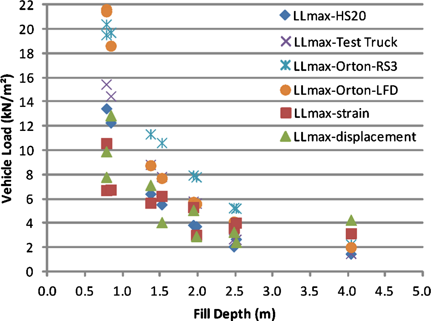
Comparison of vehicle load based on RS3, LFD, field data and calculated values.

Table 4

Vehicle load results based on RS3, LFD, field data and calculated values

Culvert	S	t	Fill Depth (Z)	E	E-Test Test Truck	Ls	L	LLmax-HS20	LLmax-Test Truck	LLmax-Orton-RS3	LLmax-Orton-LFD	LLmax-strain strain	LLmax-displacement
Name	m	m	m	m	m	m	m	kN/m²	kN/m²	kN/m²	kN/m²	kN/m²	kN/m²
A6330	13.70	0.20	0.78	1.619	2.819	3.419	3.673	13.45	15.45	20.40	21.64	6.70	7.80
N0793	9.26	0.22	0.78	1.619	2.819	3.419	3.673	13.45	15.45	19.54	21.45	10.58	9.91
L0525	8.07	0.29	0.84	1.724	2.924	3.524	3.778	12.28	14.48	19.73	18.63	6.75	12.88
N0502	14.60	0.20	1.37	2.652	3.852	4.452	4.706	6.41	8.83	11.35	8.76	5.65	7.13
N0936	7.80	0.20	1.52	2.914	4.114	4.714	4.968	5.53	7.83	10.63	7.71	6.22	4.07
X0749	7.89	0.23	1.94	3.649	4.849	5.449	5.703	3.84	5.79	7.95	5.75	5.31	5.08
A2869	7.52	0.24	1.98	3.719	4.919	5.519	5.773	3.73	5.63	7.80	5.60	3.02	2.92
R0015	8.72	0.24	2.48	13.094	10.044	6.648	6.648	2.07	2.70	5.27	4.12	3.59	3.26
N0059	6.57	0.19	2.51	8.897	10.097	6.701	6.701	2.68	2.66	5.22	4.07	4.02	2.44
P0622	7.95	0.25	4.04	11.574	12.774	9.378	9.378	1.47	1.50	2.25	2.01	3.16	4.26

In the study, the design results were close to the RS3 results, while the loads calculated from the field measurements were considerably smaller than both the RS3 and design values, especially at shallower fill depths. It was seen that load values calculated for the test truck from vehicle load formulas presented in the current study were closer to the loads from field data for much cases. Four LLmax-Test Truck result values were greater than the results of LFD method from the study, but the difference between these four results were ranged from 0.5% to 1.6%. Interestingly, HS20 truck results gave almost the same results with the load results from field data. This was owing to the fact that the test truck formulas contains 4*P_max for all cases while the HS20 truck formulas contains wheel loads ranging from 1*P_max to 4*P_max. Thus the HS20 truck formulas created smaller values than LLmax-Test Truck results.

It is also important to note that in the first study, Abdel-Karim et al. [3] placed pressure sensors on the top of the culvert while in the second study Orton et al. [7] placed strain transducers and linear variable displacement transducers under the top slabs of the culverts. Placing measurement instruments under the top slabs can cause obtaining more distributed values than placing measurement instruments on the top of culverts. Since concrete slab would distribute vehicle loads, reading exact peak values is not possible from measurement instruments under the top slabs. Therefore, because of this distribution effect, some low values can be expected from measurement instruments under the top slabs. In conclusion, formulas generated in the current study for the test trucks were consistent with the test results of both studies.

3.2.3 Impact factor for vehicle load

AASHTO SSHB also specifies an impact factor for live loads acting on span to consider dynamic, vibratory and impact effects in Article 3.8.2.3 [2]. Impact factor values for culverts are listed in Table 5.

Table 5
Impact factor table [2]

Fill Depth Interval Impact Factor I

Z ≤ 0.3 m 1.3

0.3 m <Z ≤ 0.6 m 1.2

0.6 m <Z ≤ 0.9 m 1.1

0.9 m <Z 1

Fill Depth Interval	Impact Factor I
Z ≤ 0.3 m	1.3
0.3 m <Z ≤ 0.6 m	1.2
0.6 m <Z ≤ 0.9 m	1.1
0.9 m <Z	1

3.2.4 Lateral surcharge load

According to the AASHTO SSHB Article 3.20.3, minimum 0.6 m (2 ft.) lateral earth pressure shall be applied to exterior walls of the culvert, when traffic can come from a distance equal to one half of the culvert height [2]. Live load surcharge was not considered for depth of fill values greater than 2.44 m (8 ft.) as stated in the ASTM C890-13 Article 5.5.2 [9]. Live surcharge load was calculated from the following equation as stated in the AASHTO SSHB Article 5.5.2: [2] $LS = K_{0} γ 0.6 ({kN / m}^{2})$ (29)

3.3 Load combinations

The following load combinations were used in the analysis of culvert models to evaluate maximum internal forces: $1.30 \times (DL + EP + 1.67 \times LS + 1.67 \times I \times LL)$ (30)

$\begin{matrix} 1.30 \times (DL + 0.5 \times EP + 1.67 \times LS + 1.67 \\ \times I \times LL) \end{matrix}$ (31) $DL + EP + LS + I \times LL$ (32)

The first two combinations are listed in the AASHTO SSHB Table 5.22.1A [2]. No load factors were used in the third combination except the impact factor.

4 Finite element modeling and analysis

The modelling process was automated by developing a Microsoft Excel sheet by using VBA and Computers and Structures Inc. Application Programming Interface [11]. 2D structural-frame finite element analysis method has high precision and accuracy for predicting moment values at the top exterior wall corners and the top midspans of culverts [6]. Thus, 2D structural-frame linear finite element analysis method was used in this study to analyze large quantities of culvert models efficiently. Springs that were used to model base soil were placed with 25 cm or lesser spacing and this spacing value was calculated as one fifteen of span width (S/15 ≤ 25). Vehicle loads were moved step by step and distributed vehicle loads were moved each step by a value equals to spring spacing. Locations of distributed vehicle loads were checked at each step and only portion of distributed vehicle load that was in the range of the span was considered for loading. An example vehicle loading step is shown in Fig. 9.

Fig.9

Wheel load projections and equivalent distributed vehicle loads.

After typing material properties and section properties in the Excel sheet, loads and 2D finite element structural-frame model were automatically created in SAP2000 version 17.2.0 [12]. With the completion of analysis, results were transferred from SAP2000 to the Excel sheet. Maximum and critical internal forces and soil stress were gathered in a table and base soil stress diagram was drawn automatically.

5 Analysis results

An example moment diagram, which was produced for a double cell RCBC by SAP2000, is shown in Fig. 10. As it can be seen in this figure, while positive moment occurrence was clear at base and top slabs, positive moment did not occur for much cases at wall sections.

Fig.10

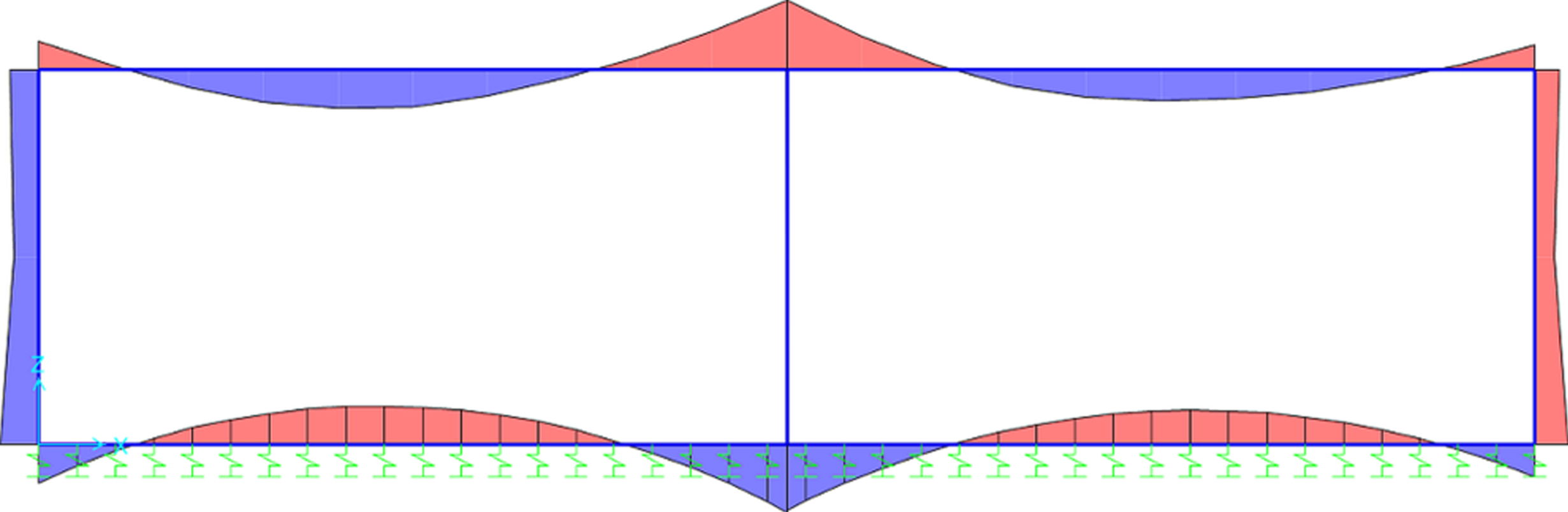
Moment diagram for a double cell RCBC.

Table 6 shows the analysis results of box culvert models. Maximum and critical internal forces and soil stress are shown in this table where Mt, Mw, and Mb are the maximum moment results of top slab, walls and base slab, respectively. Vt, Vw, and Vb are maximum shear force results of top slab, walls and base slab. qs shows maximum base soil stress results. Negative moment was considered for walls and base slab, positive moment was considered for top slab in Table 6 and in figures that show moment graphs. Moments that produce tension in the bottom fibers of slabs and in the inner fibers of walls were taken into account as positive moment.

Table 6

Analysis results of RCBC models

Group	Case	No	Mt	Mw	Mb	Vt	Vw	Vb	qs
			kNm	kNm	kNm	kN	kN	kN	kN/m²
1. Group	WIDTH CASE I Z = 0.5 m	1	–1.420	14.608	0.953	50.466	45.450	58.132	117.066
		2	13.057	18.451	17.627	97.955	45.585	102.394	100.573
		3	43.406	29.832	34.311	142.774	44.460	138.712	124.119
		4	75.538	53.327	43.368	171.394	43.242	157.171	137.207
		5	110.012	82.165	58.497	193.371	47.584	179.697	130.876
		6	107.701	102.956	84.104	217.455	51.002	211.769	120.398
		7	230.061	227.271	139.876	297.339	65.541	297.498	135.995
		8	388.147	468.162	203.355	392.583	104.734	402.786	148.256
	WIDTH CASE II Z = 0.7 m	9	–4.917	15.041	4.435	27.016	48.261	36.253	82.891
		10	3.825	16.307	7.075	53.580	48.428	61.125	67.078
		11	23.515	22.157	21.020	84.673	47.940	87.744	76.676
		12	45.869	36.863	28.939	108.478	46.877	104.564	92.511
		13	71.683	57.823	41.672	129.105	47.640	125.770	95.864
		14	77.381	77.376	61.999	151.123	50.791	153.203	95.071
		15	168.874	171.443	105.037	214.530	56.924	222.326	111.409
		16	300.855	359.509	159.990	296.030	84.910	313.190	126.008
	WIDTH CASE III Z = 1.5 m	17	–7.612	18.499	7.124	20.105	59.494	29.812	79.078
		18	–0.339	18.444	2.531	40.209	59.678	48.737	64.166
		19	16.443	23.826	17.789	66.651	59.872	72.911	62.719
		20	39.625	36.776	31.615	97.624	57.509	97.263	88.067
		21	68.731	62.472	48.284	128.944	54.793	127.134	103.164
		22	101.275	96.622	68.902	159.654	56.889	160.986	111.442
		23	189.555	202.174	118.534	229.274	71.786	236.598	127.730
		24	347.715	424.742	181.856	328.713	106.694	344.064	148.177
	WIDTH CASE IV Z = 3.0 m	25	–5.466	20.892	4.983	27.909	66.485	37.099	103.631
		26	3.719	21.336	7.042	55.818	66.663	63.289	88.501
		27	26.322	29.063	26.909	93.030	66.718	97.150	92.020
		28	59.538	50.117	46.242	139.545	63.158	133.944	135.974
		29	103.000	89.528	74.448	188.296	62.121	179.309	156.375
		30	154.943	144.762	104.441	236.815	69.655	229.769	170.007
		31	284.780	304.264	168.935	334.908	92.873	333.083	190.449
		32	504.907	609.748	257.642	463.445	140.563	470.205	210.509
2. Group	HEIGHT CASE I Z = 0.5 m	33	11.860	9.097	12.103	82.404	7.439	79.717	90.882
		34	13.074	8.326	13.561	82.404	13.677	81.526	94.042
		35	13.110	9.242	13.902	82.404	23.239	83.804	97.666
		36	11.719	12.287	12.754	82.404	34.813	86.104	100.889
		37	8.931	17.720	10.072	82.404	48.415	88.427	103.932
		38	4.687	25.885	5.728	82.404	64.052	90.777	108.291
		39	–1.111	37.172	0.448	82.404	81.728	93.157	113.139
		40	–8.579	51.988	8.644	82.404	101.445	95.572	118.359
	HEIGHT CASE II Z = 0.7 m	41	6.366	5.241	6.654	44.793	8.209	44.652	57.457
		42	6.764	5.324	7.302	44.793	14.887	46.469	60.501
		43	6.090	7.029	6.944	44.793	25.020	48.756	64.008
		44	4.154	10.747	5.257	44.793	37.172	51.062	67.260
		45	0.892	16.826	2.108	44.793	51.355	53.391	71.413
		46	–3.799	25.661	2.677	44.793	67.574	55.748	76.000
		47	–10.041	37.662	9.293	44.793	85.833	58.135	80.920
		48	–17.969	53.254	17.942	44.793	106.133	60.557	86.221
	HEIGHT CASE III Z = 1.5 m	49	4.669	4.182	4.971	33.508	11.038	34.132	53.769
		50	4.690	4.785	5.245	33.508	19.581	35.954	56.737
		51	3.497	7.342	4.372	33.508	32.050	38.249	60.085
		52	0.923	12.214	2.052	33.508	46.540	40.567	63.784
		53	–3.129	19.786	1.880	33.508	63.063	42.911	68.247
		54	–8.778	30.472	7.616	33.508	81.622	45.285	73.037
		55	–16.156	44.695	15.357	33.508	102.220	47.694	78.202
		56	–25.401	62.884	25.313	33.508	124.861	50.142	83.791
	HEIGHT CASE IV Z = 3.0 m	57	6.598	5.590	6.884	46.515	12.763	46.260	78.565
		58	6.978	6.100	7.515	46.515	22.481	48.081	81.535
		59	6.211	8.856	7.063	46.515	36.413	50.377	84.774
		60	4.104	14.224	5.206	46.515	52.363	52.700	88.168
		61	0.597	22.569	1.814	46.515	70.344	55.051	92.793
		62	–4.414	34.290	3.289	46.515	90.361	57.436	97.799
		63	–11.049	49.804	10.294	46.515	112.417	59.857	103.231
		64	–19.442	69.536	19.405	46.515	136.515	62.320	109.137
3. Group	ONE CELL Z is 0 to 5 m	65	346.979	417.881	185.218	357.609	90.293	369.995	130.769
		66	388.147	468.162	203.355	392.583	104.734	402.786	148.256
		67	300.855	359.509	159.990	296.030	84.910	313.190	126.008
		68	305.225	370.583	161.634	294.686	91.034	312.104	130.761
		69	399.853	486.841	206.404	371.334	122.665	384.021	168.026
		70	504.907	609.748	257.642	463.445	140.563	470.205	210.509
		71	634.153	766.792	319.089	582.508	180.120	581.462	260.764
		72	772.045	934.226	384.640	709.502	221.398	700.125	313.731
	DOUBLE CELL Z is 0 to 5 m	73	116.161	121.187	110.779	219.152	67.085	215.025	82.218
		74	122.920	127.821	118.288	237.396	72.936	228.744	89.156
		75	88.465	102.332	89.889	177.247	72.655	180.260	74.834
		76	83.053	97.510	87.802	173.701	71.610	183.413	75.007
		77	94.892	108.352	103.550	210.942	80.390	231.257	88.698
		78	117.963	126.431	125.229	263.036	81.006	283.676	106.611
		79	147.835	152.592	153.973	329.396	94.694	350.036	128.977
		80	179.734	180.312	184.659	400.207	108.361	420.847	152.546
	TRIPPLE CELL Z is 0 to 5 m	81	68.705	75.525	62.144	157.228	64.881	165.506	80.213
		82	71.011	78.106	65.454	168.468	70.864	172.696	86.379
		83	50.577	64.159	48.524	119.212	70.655	133.488	72.717
		84	44.125	58.329	47.159	123.770	69.404	125.973	72.654
		85	46.054	60.027	53.635	142.897	78.861	146.899	84.595
		86	57.949	67.555	64.637	176.738	79.569	177.516	100.689
		87	72.469	80.050	79.007	220.528	93.583	217.820	120.955
		88	88.003	93.168	94.376	267.280	107.597	260.849	142.307

5.1 Effect of span width

Figure 11 shows the variation of maximum moment and shear force, which were occurred at top slab and maximum base soil stress with respect to span width. As expected internal forces were increasing as span width was increasing. Internal forces of Case II had lowest values at over 4 m span width. Although fill depth was 3 m for Case IV and 0.5 m for Case I, internal forces of Case IV were lesser than internal forces of Case I at 0.6 m to 4 m span width range. This was due to the fact that Case I had a greater distributed vehicle loads. After 4 m span width value, while Case I had limited vehicle load distribution width (E1 <2.13 m), Case IV vehicle loads were distributed over whole span width. Thus, Case IV internal forces overtook internal forces of Case I after 4 m span width with contribution of 3 m fill depth.

Fig.11

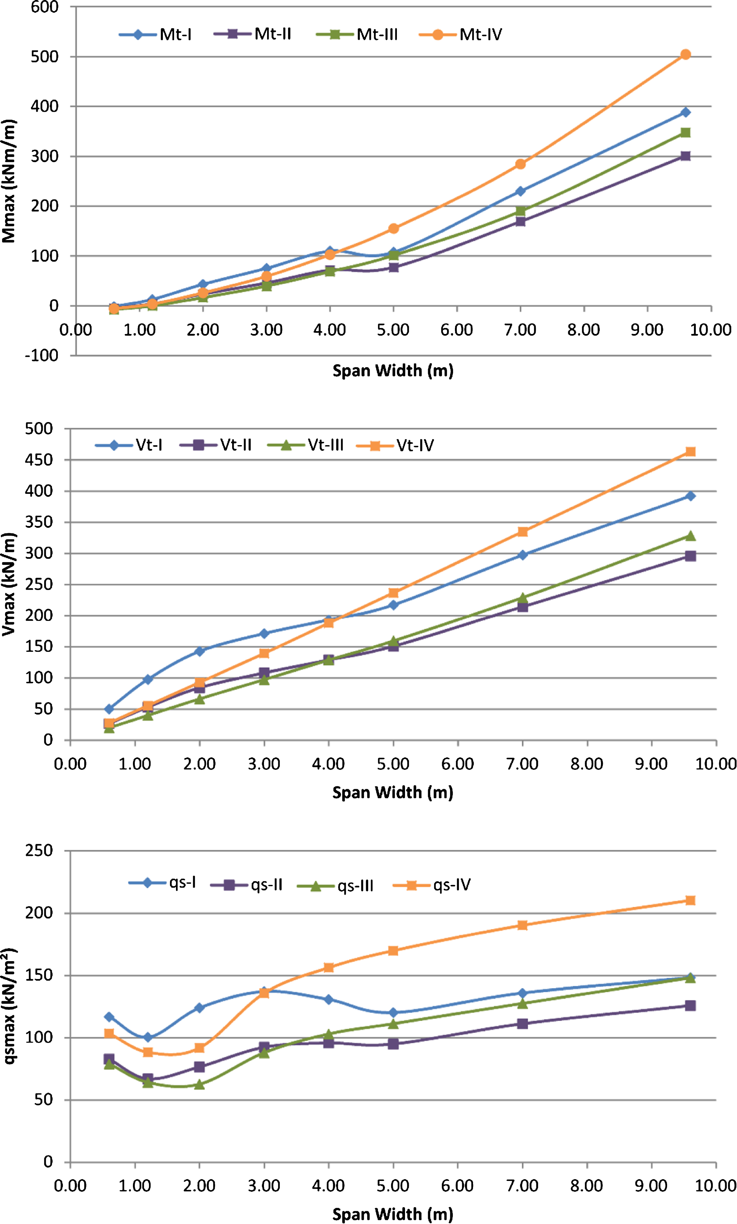
Internal forces and base soil stress with respect to span width.

The same trend is valid for base soil stress graph, but slope of this graph is increasing more slowly than internal forces. Increasing base area of the culvert as span width increasing caused to limited increase in base soil stress. As base soil stress is inversely correlated with base area of structures. After 3 m span width value, base soil stress of Case IV overtook base soil stress of Case I.

5.2 Effect of culvert height

Figure 12 shows the variation of maximum moment and shear force which were occurred at exterior walls and maximum base soil stress with respect to culvert height. Since increment at culvert height caused lateral earth pressure to increase according to Equation 6, internal forces at exterior walls were increasing, too. Similar to Fig. 11, moments of Case IV were lesser than moments of Case I at 0.6 m to 2 m culvert height range. This is due to the fact that Case I had a greater distributed vehicle loads and moment continuity between top slab and walls increased moment values at walls. Besides, soil pressures of Case IV were lesser than soil pressures of Case I at all culvert height values. In contrast to these trends, shear force values of Case IV were greater than other cases, because shear forces at walls were affected directly by the lateral earth pressure.

Fig.12

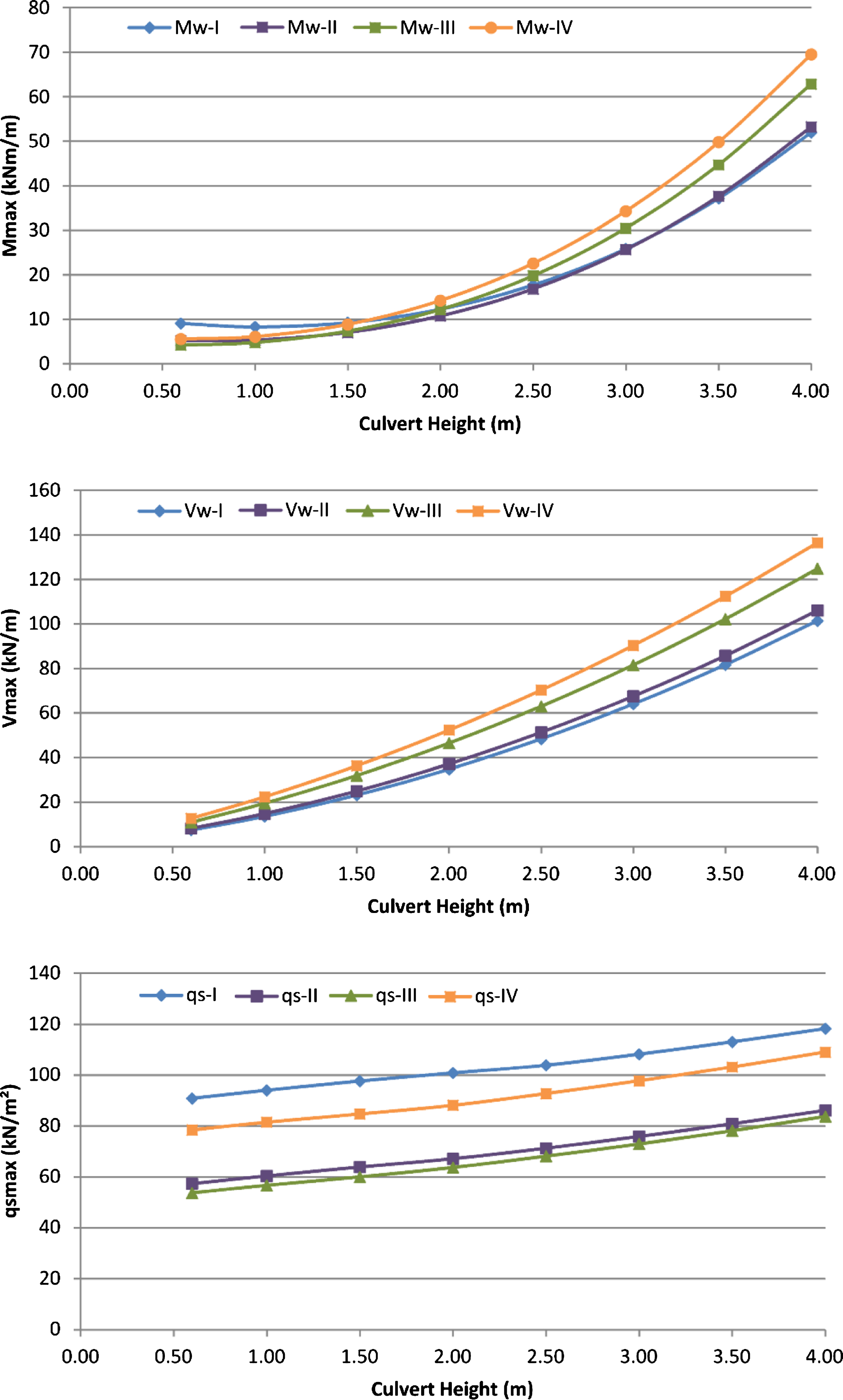
Internal forces and base soil stress with respect to culvert height.

5.3 Effect of fill depth

Variation of maximum moment, shear force and base soil stress with respect to fill depth is shown in Fig. 13. Internal forces were increasing generally with the increment of fill depth for one cell, double cell and triple cell culvert models. Internal forces were decreasing after 0.60 m fill depth since distributed vehicle load starts to decrease sharply at this fill depth as shown in Fig. 13. Internal forces and base soil pressures reached their minimum values at 0.70–1.0 m fill depth range. After 1 m of fill depth, as vertical earth load was overtaking vehicle load, internal forces were starting to increase again. Double and triple cell culvert models had close results while one cell culvert models had greater internal forces. Slopes of internal force graphs for one cell culverts were much greater than slopes of internal force graphs for double and triple cell culverts.

Fig.13

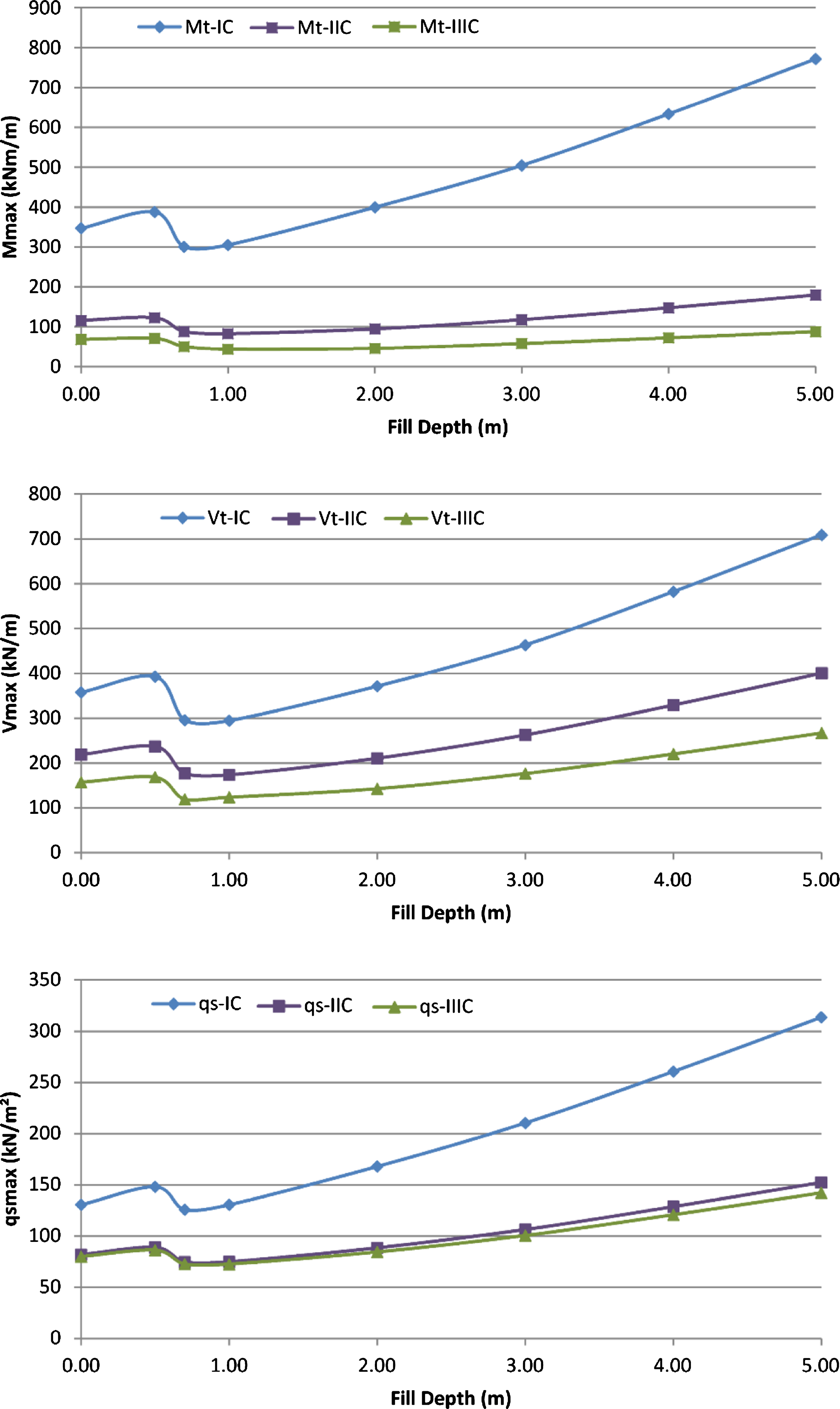
Internal forces and base soil stress with respect to fill depth.

6 Conclusions and recommendations

In this study, derivation of vehicle load distribution formulas are explained in detail and verified by comparison with experimental studies. Analysis and design procedures of RCBC were explained. 88 finite element culvert models were created by using SAP2000. A Microsoft Excel sheet was developed by using VBA and CSI API to create SAP2000 models automatically. Effects of span width, culvert height and fill depth on RCBC design were investigated.

It was observed that span width is an important parameter for RCBC as it dramatically increased internal forces and base soil pressures of culvert models in the first model group.

It can be concluded that culvert height is an effective parameter for internal forces of wall members from the second model group results. However, it is not effective for base soil pressures, since it did not affect base soil pressures significantly. Therefore, it can be observed that culvert height is not an important parameter unlike span width or fill depth for culvert design.

The third model group results indicated that fill depth has an important effect on both internal forces and base soil pressures. The results for the third model group showed that vehicle load has a significant effect on the internal forces of culverts especially at lower fill depth values and while vehicle load was predominant for fills that did not have a depth value greater than 1 m, vertical earth load was predominant beyond 1 m fill depth. Since minimum values of internal forces and base soil pressures occurred at 0.70–1.0 m fill depth range, it can be concluded that designing RCBC with a fill depth value in the range of 0.70–1.00 m is preferred for more economical and reliable designing.

Adding interior walls to wider single cell culvert models for obtaining multiple cell culverts greatly decreased internal forces and base soil pressures. Even analysis results of double cell culverts were much smaller than the results of single cell culverts. Since moment results of multiple cell RCBC were lower, multiple cell RCBC need lesser reinforcement area. It must also be noted that equal section thicknesses were used to create same conditions for single, double and triple cell culvert models in the third model group. However, section thickness can be reduced for multiple cell culverts in practice since their actual effective span width values are smaller than single cell culverts. Besides, single cell RCBC can need base soil improvements due to higher base soil pressures. Therefore, using multiple cell culverts instead of using wider span width in single cell culverts is a more reliable choice because of lesser reinforcement area, smaller section thickness and lower base soil pressure.

References

Culvert Materials Chapter in Drainage Manual [Internet]. Connecticut Department of Transportation; 2000. Available from: http://www.ct.gov/dot/cwp/view.asp?a=1385&Q=260090

Standard Specifications for Highway Bridges (17th ed.). Washington, DC: American Association of State Highway and Transportation Officials; 2002.

Abdel-Karim

, Tadros

, Benak

. Live load distribution on concrete box culverts. Transportation Research Record. 1990;(1288):136–51.

Chen

, Zheng

, Han

. Experimental Study and Numerical Simulation on Concrete Box Culverts in Trenches. Journal of Performance of Constructed Facilities. 2010;24:223–34. doi:10.1061/(ASCE)CF.1943-5509.0000098

Pimentel

, Costa

, Félix

, Figueiras

. Behavior of reinforced concrete box culverts under high embankments. Journal of Structural Engineering. 2009;135:366–75. doi:10.1061/(ASCE)0733-9445(2009)135:4(366)

Wood

, Lawson

, Jayawickrama

, Newhouse

. Evaluation of production models for load rating reinforced concrete box culverts. Journal of Bridge Engineering. 2015;20. doi: 10.1061/(ASCE)BE.1943-5592.0000638

Orton

, Loehr

, Boeckmann

, Havens

. Live-load effect in reinforced concrete box culverts under soil fill. Journal of Bridge Engineering. 2015;20:04015003. doi:10.1061/(ASCE)BE.1943-5592.0000745

Jaky

. The coefficient of earth pressure at rest. Journal of the Society of Hungarian Architects and Engineers. 1944;78(22):355–8.

Standard Practice for Minimum Structural Design Loading for Monolithic or Sectional Precast Concrete Water and Wastewater Structures. C890-13. West Conshohocken, PA: American Society for Testing and Materials; 2013.

10.