
Abstract
Rail-structure interaction (RSI) analysis and vehicle-track-structure-interaction (VTSI) analysis are often required during bridge design. For example, the California High-Speed Train Project requires RSI analysis for final design of all structures, as well as VTSI analysis, with the level of interaction to be modeled determined by the complexity of a structure. The goal of RSI analysis is to ensure that superstructure deformations and rail stresses are within acceptable limits. VTSI analysis is a dynamic analysis that takes into account influence of actual trainsets. VTSI Level 1 analysis includes train loads as a series of moving loads. This analysis allows evaluation of dynamic impact effects from trainsets and vertical accelerations of the deck. For complex high-speed railway bridges, VTSI Level 2 might be required, accounting for full dynamic interaction between the trainset and the bridge. To represent this interaction, the trainset is modeled as a multibody system consisting of rigid bodies, springs, and dashpots. The interaction between wheels and rails is accounted for through kinematic constraints and Lagrange multipliers. This paper presents modeling, RSI, and VTSI analyses of a railway bridge in the LARSA 4D software package. The track and superstructure are modeled in an expedited way using a macro that generates the track, approach, and bridge geometries. Fasteners are modeled as hysteretic springs and automatically positioned along the curved geometry of the track using a LARSA 4D’s bridge path coordinate system definition. RSI analysis is performed accounting for temperature differentials between rails and the deck, vertical train loads, acceleration and braking forces. Break in the rail is introduced using stage construction analysis, followed by progressive collapse analysis (with adapting increments and arc-length control) or nonlinear dynamic analysis. Finally, VTSI Level 1 and 2 analyses are performed and the results are compared. Car body accelerations are compared to limit values to ensure passenger comfort.
Keywords
Introduction
The interaction between a track and a structure became an important part of designing railway structures due to the introduction of continuously welded rails (CWR). Such rails lack joints and, therefore, temperature variations can generate excessive stresses in rails, which in turn cause additional deformations in structures. The goal of rail-structure interaction (RSI) analysis is to limit structure deformations at expansion joints and limit axial rail stresses. Track-structure interaction requirements for bridges depend on the type of railway track. For example, while the United States does not have a national design code for light-rail transit bridges, many local codes were developed that specify the requirements for RSI analysis of such structures (see Okelo et al. [1]). A comparison of such codes was performed by Ahlbeck et al. [2]. They found out that different organizations took substantially different engineering approaches in designing railway structures with CWR. At high train speeds, the response of the bridge can be amplified due to the reciprocal influence of the structure and the trainset on each other, which may lead to resonance. The trainset applies a load on the bridge, and bridge deformation acts as support excitation for the trainset, in turn affecting the load. Therefore, not only RSI but also vehicle-track-structure-interaction (VTSI) should be taken into account. As an example of a design code for high-speed railway tracks, the California High-Speed Train Project (CHSTP) developed a technical memorandum TM 2.10.10: Track-Structure Interaction [3]. The requirements outlined in this code limit bridge deformations and accelerations to avoid excessive rail stresses, derailments, and passenger discomfort. In Europe, Eurocode EN 1991-2 [4] sets standards for both RSI and VTSI analyses, and UIC Code 774-3 [5] provides recommendations for calculations for RSI analysis. In Japan, “Design Standards for Railway Structures and Commentary” for concrete [6] and steel-concrete [7] structures are used.
The present work is focused on modeling and analysis methods that apply to RSI and VTSI analyses. This paper aims to give an overview of the practical implementation of these analyses in standard structural analysis software.
Modeling
Description of the model
The two-track bridge used in this study consists of 6 spans of 40 m (see Fig. 1). The first three spans are straight, while the last three spans are curved with a radius of 274 m. The superstructure consists of a box girder. The rails are continuous over the structure and approaches. Expansion bearings are used at Pier 3 and abutments.
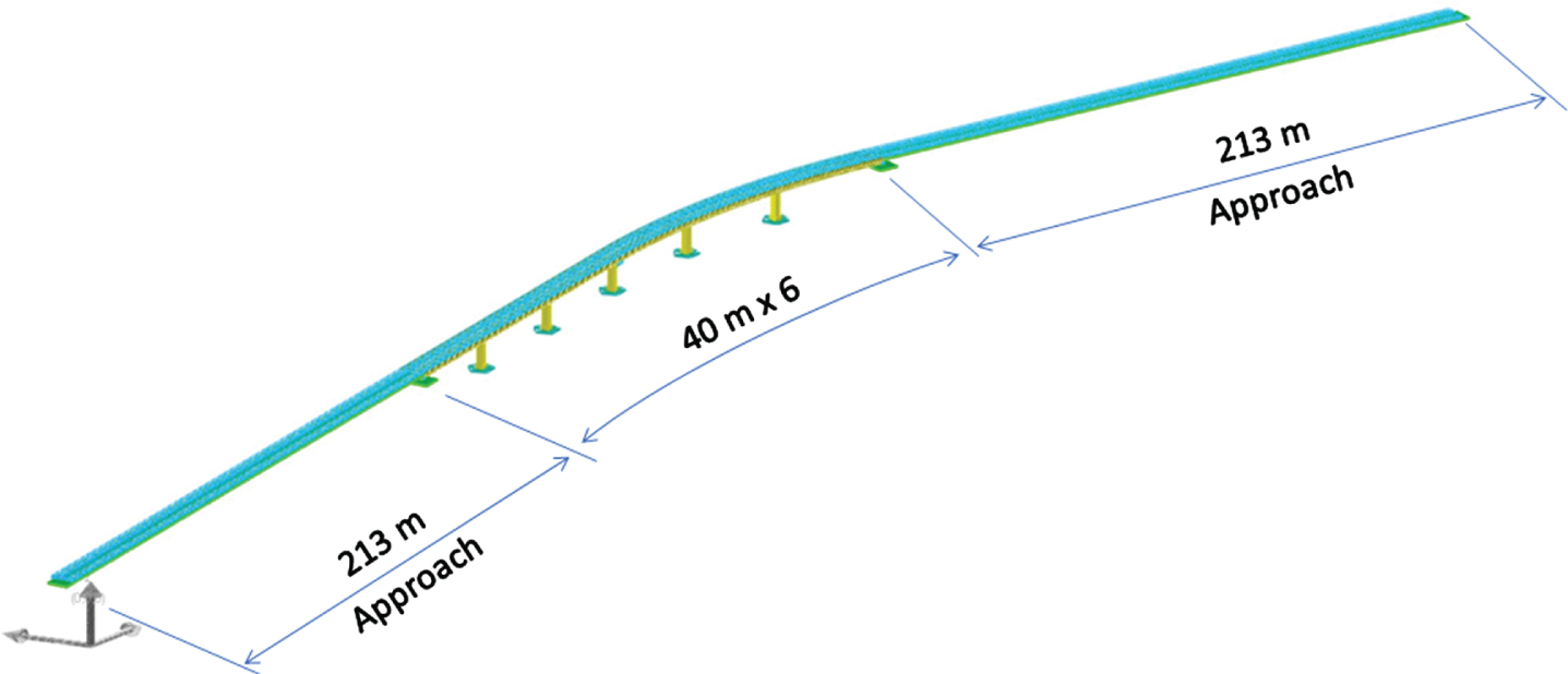
Model of a 6-span bridge with approaches.
It is specified in TM 2.10.10 [3] that the rails should be extended beyond the structure for at least (0.1Lavg+99) m = 103 m, where Lavg is an average span length. At the same time, elastic-perfectly plastic springs should be used at the ends of approaches to model boundaries (see Section 2.3 for spring properties). The yielding of these springs should be checked throughout the analysis and, if they yield at any point, the length of approaches should be increased. Calcada et al. [8] performed analyses on a similar type of bridge and noted that a necessary length of a modeled approach should be at least 198 m. In this model, the track is extended 213 m beyond the bridge on each side.
For the purposes of VTSI analysis in this paper, in Sections 4 and 5 the bridge model is assumed to be straight.
The bridge is modeled in the structural analysis software package LARSA 4D. The model is created in an expedited way using a macro that generates track, approach, and bridge geometries. The macro was developed in MS Excel to streamline the generation of rail-structure interaction models that typically contain a large number of repeating elements, such as springs representing fasteners and ballast, as well as rigid links, which are used to position rail members with respect to the deck (see Fig. 2).
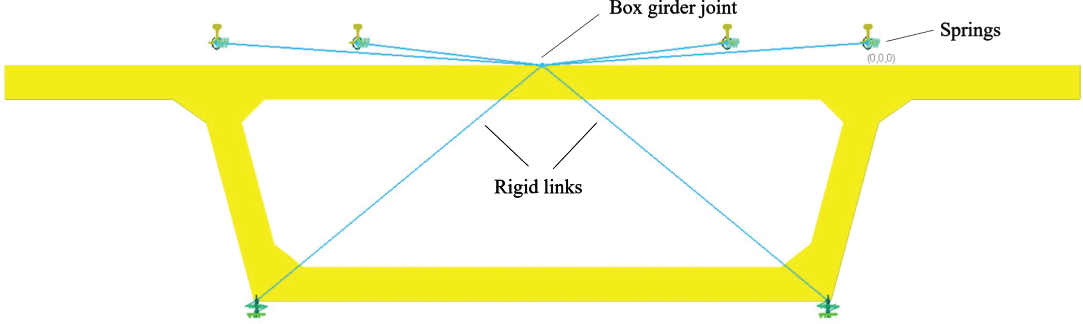
The connection between the superstructure and the rails.
The macro takes as inputs the length of the bridge and approaches, the number of tracks, the distance between the tracks, the distance between the rails of a track, the longitudinal distance between fasteners, and the relative height of the rails with respect to the deck. The deck and rails are then generated. At the position of the rail, two repeated nodes are generated for each fastener. Horizontal springs are generated between these nodes to model fasteners. Similarly, vertical springs can be generated to model the vertical stiffness of fasteners or ballast in the case of ballasted tracks. Using the LARSA Section Composer tool, the box girder section is created, and its centroid is offset from the reference axis (the axis connecting member’s joints). Rigid links are then used to connect girder joints to springs’ joints. The bridge path coordinate system is then created to generate the curved alignment of the bridge.
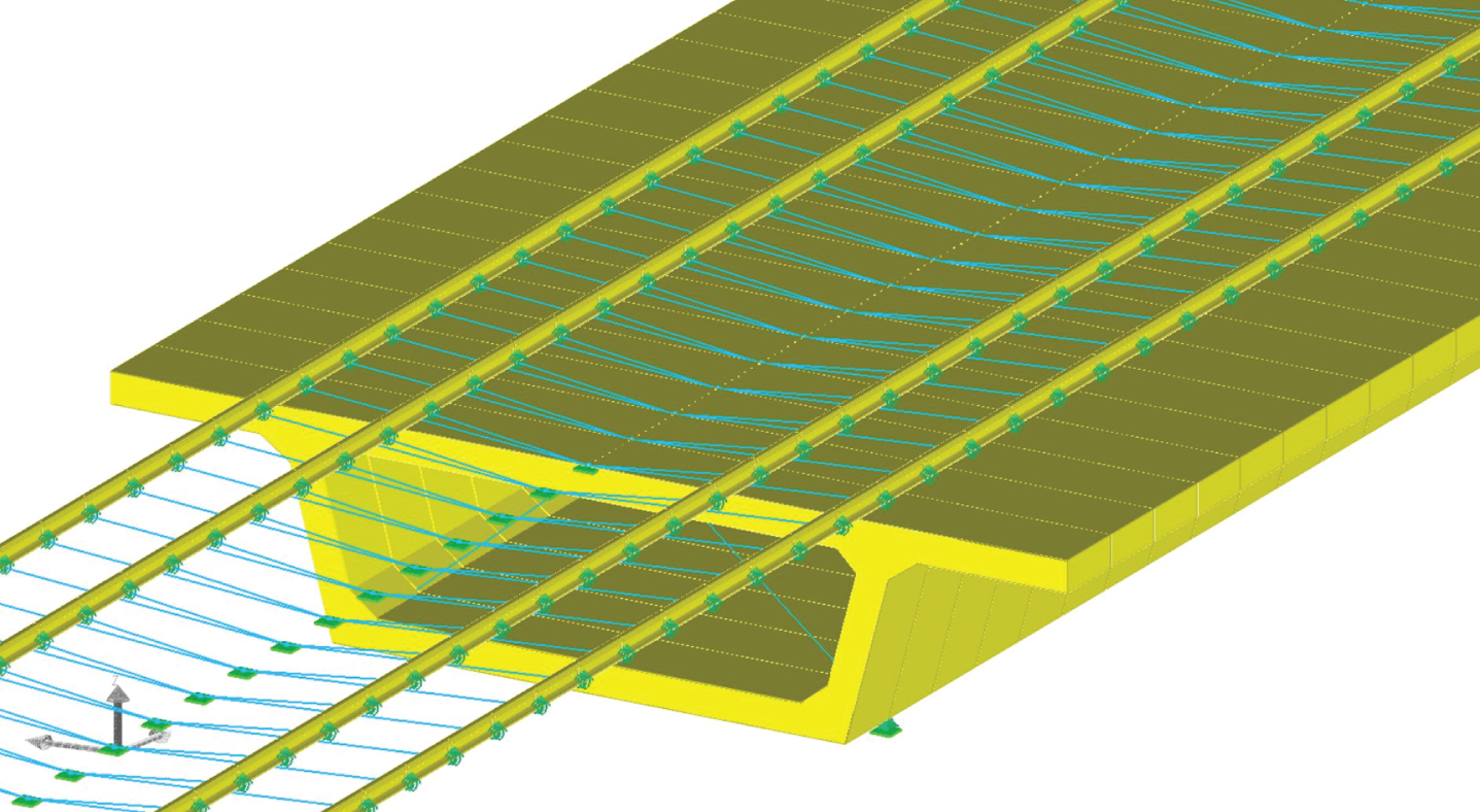
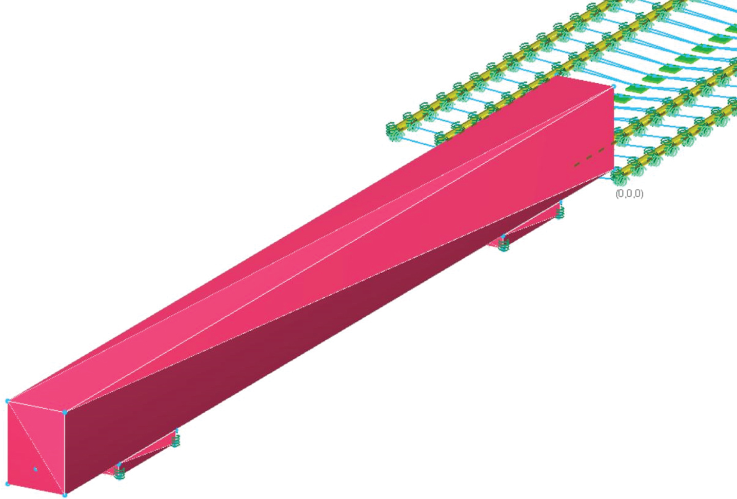
Isometric view of two tracks over the approach and bridge.
Material and section properties are presented in Tables 1 and 2 correspondingly. Section properties are calculated automatically based on the geometry defined in the Section Composer tool. The first frequency of the bridge is 1.87 Hz.
Material properties
Material properties
Section properties
The properties of rail fasteners are selected per CHSTP TM 2.10.10 [3]. The track-deck connection force-displacement behavior in the longitudinal direction is approximated using a bilinear function. The yield displacement for this function is 0.51 mm for the non-ballasted track on the bridge and 2.03 mm for ballasted track on approaches. The stiffness of the track’s longitudinal restraint depends on the level of vertical load. Since we account for the vertical train loads, we assume that the track is loaded and use the corresponding value for the longitudinal restraint, which equals 39.4 kN per meter of track. The track-deck connection in the longitudinal direction is modeled with discrete hysteretic (inelastic) springs positioned at 0.76 m. Therefore, the yield force of each longitudinal spring is 15 kN. The spring properties are presented in Figs. 4 and 5.
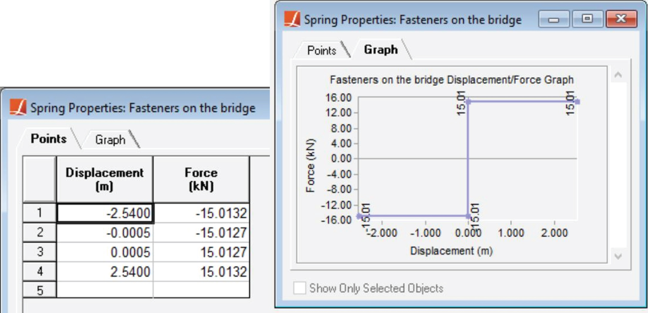
Properties of a hysteretic spring representing the longitudinal stiffness of fasteners located over the bridge.
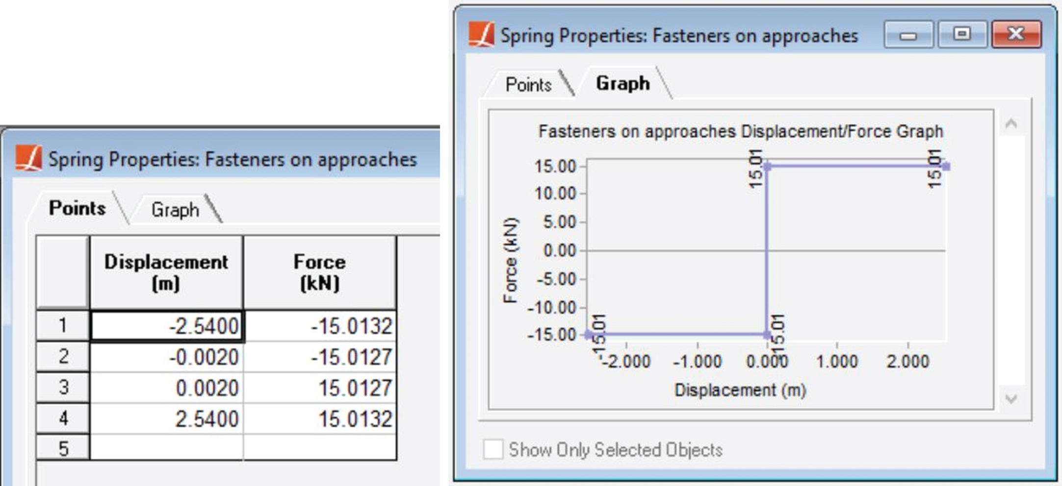
Properties of a hysteretic spring representing the longitudinal stiffness of fasteners located over the approaches.
Boundary springs should be used at the model boundaries (at the ends of approaches), according to TM 2.10.10 [3]. These springs represent an infinite number of fasteners. Spring properties are selected according to the design code and presented in Fig. 6.
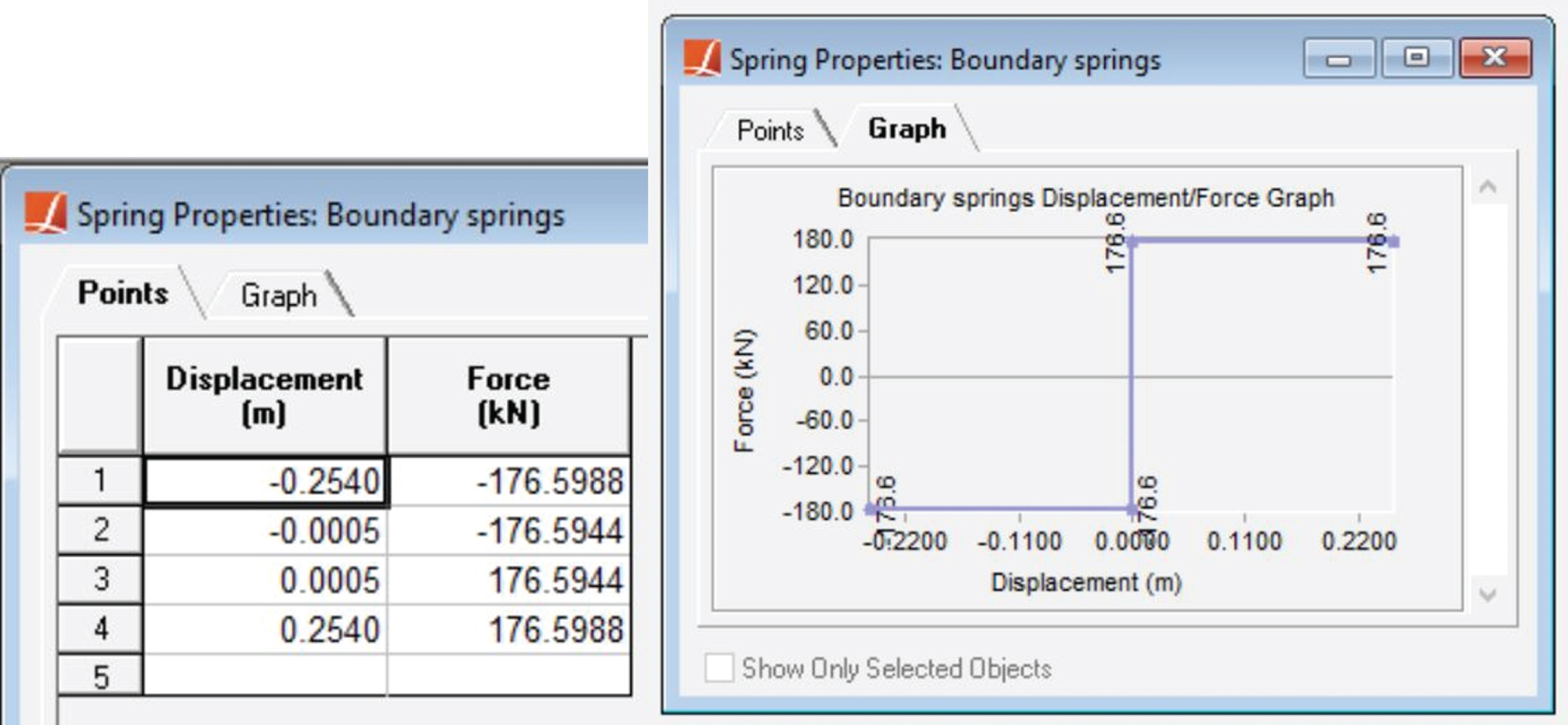
Properties of a boundary spring.
According to CHSTP TM 2.10.10 [3], constant vertical stiffness should be used to model fastener compression and tension. Therefore, linear springs are used to represent the vertical stiffness of fasteners. The spring stiffness is equal to 196 MN/m per meter of track (74.7 MN/m per fastener) for the non-ballasted track over the bridge and 100 MN/m per meter of track (38.7 MN/m per fastener) for the ballasted track over the approaches. The lateral stiffness of fasteners is modeled with a linear spring as well and is equal to 20 MN/m per meter of track (7.7 MN/m per fastener) over the whole length of the tracks.
Loading
In this study, we are following the requirements of CHSTP TM 2.10.10 [3]. The model is analyzed for one of the two required RSI load cases. Namely, the load case Group 4, which consists of the following loads: (LLRM + I)2 + LF2±TD, where
(LLRM + I)2 = two tracks of Modified Cooper E-50 (LLRM) (see Fig. 7) plus vertical impact effect I from LLRR (Maintenance and construction train live load);
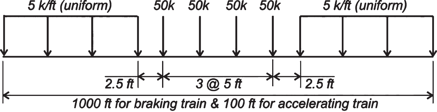
Modified Cooper E-50 loading (CHSTP TM 2.10.10 [3]).
LF2 = braking and acceleration forces (applying braking to one track, acceleration to the other track) for LLV (Actual high-speed train) loading;
TD = temperature differential of ± 22.2°C between rails and deck, applied to the superstructure.
The vertical impact effect I from LLRR (Maintenance and construction train live load) is computed according to TM 2.3.2: Structure Design Loads [9]. For spans over 38 m, the impact factor I is equal to 20%. The applied vertical load is increased by that factor accordingly.
Braking and acceleration forces from high-speed trains are computed per TM 2.3.2 as well. Acceleration force is taken to be 32.98 L (kN), where L is the length in meters of a portion of the bridge under consideration. The braking force is equal to 19.99 L (kN). We assume L to be equal to the length of the train. The loads should be distributed over the length of the train. The load pattern of Modified Cooper E-50 is used to generate these loads.
According to UIC Code 774-3, the influence of each component of interaction should be evaluated separately. The simple sum of the contributions (even though the analyses are nonlinear) is then compared to the overall effects. Therefore, we start by performing three separate analyses based on the loads described above. The stage construction analysis is then performed, where the results of each analysis are retained before applying additional loads and performing the subsequent analysis.
The Modified Cooper E-50 loading and braking and acceleration loads are applied in two separate Moving Load Analyses. In both cases, lanes corresponding to each rail are created to define paths for the loads. The load patterns are then generated based on loading in Fig. 7. Finally, the load cases are created taking into account the direction of loading, initial positions of trains, and forward increments. The moving load analysis then automatically generates all the load cases for train positions along the track and performs linear static analysis on each generated case. It should be noted that since the analysis is linear, all the nonlinear elements, such as hysteretic springs, are treated as linear elements during this analysis. Since RSI is inherently nonlinear, once the most critical position of the vehicle is obtained through the moving load analysis, a nonlinear analysis should be performed on the most critical case. The third analysis is a nonlinear static analysis that evaluates the effect of a temperature drop of – 22.2°C in the superstructure. The load is applied in eight increments of – 2.78°C using the stage construction analysis.
Results
Relative longitudinal displacements at expansion joints should be limited to avoid excessive rail stresses. The obtained displacements are listed in Table 3. As described in the previous section, we first perform linear moving load analyses to determine the most critical position of the vehicle loading. Vehicle loads are then applied to the structure according to the obtained position and nonlinear static analysis is performed. The superposition of the results of the three nonlinear cases is presented in Table 3. Finally, the stage construction analysis is performed to evaluate the overall effect of all the loads.
Relative longitudinal displacements at expansion joints
Relative longitudinal displacements at expansion joints
Axial rail stresses
TM 2.10.10 [3] provides the following limit value for non-ballasted track and Group 4 load case: (0.7+δTD,exp) in, where
δTD,exp =α(ΔT)LTU – expected relative longitudinal displacement due to temperature differential,
α= coefficient of thermal expansion for the superstructure,
ΔT = 22.2°C temperature,
LTU = length of structural thermal unit for a given expansion joint.
In our model, the length of the structural thermal unit is equal to the length of three spans 119 m, and the coefficient of thermal expansion is given in Table 1 and is equal to 9.9*10–6 (1/°C). Therefore, δTD,exp is equal to 26 mm and the limit value is 44 mm. The obtained displacements are below the limit.
Axial rail stresses should be limited to avoid rail fracture. The obtained values are listed in Table 4. As per TM 2.10.10 [3], for non-ballasted track and Group 4 load case, the permissible range of additional axial rail stresses is – 96.5 MN/m2≤σrail≤ +96.5 MN/m2. The axial rail stresses at Abutment 1 and Pier 3 are above the limit if the effects of the three load cases are superposed. However, the axial rail stresses obtained through the stage analysis are within the limits. The stresses in the stage analysis are lower since the loads from the three load cases are applied gradually one after another, and the effect of yielding of springs representing fasteners is taken into account along the way. By the time the vehicle loads are applied, some of the springs have yielded due to the effect of the thermal load being applied to the deck. This allows slippage of the rails with respect to the structure and overall reduction of axial rail stresses. As mentioned in Section 2.3, inelastic springs are used to model fasteners. The yielding is determined by the yield force defined in spring properties (see Figs. 4–6 for the force-displacement relationships assigned to springs). Once a spring has yielded, it stops carrying the load. In general, if the loading is reversed or removed, the spring might become “active” again.
A rail break may occur when a temperature drop causes excessive tensile forces in the rail. The most common location for a rail break is at expansion joints, where the axial rail stresses are the largest, as can be seen in Fig. 8. The goal of evaluating the severity of a rail break is to reduce the probability of a train derailment and limit the forces redistributed to the superstructure as a result of the break (see Ahlbeck et al. [2]).
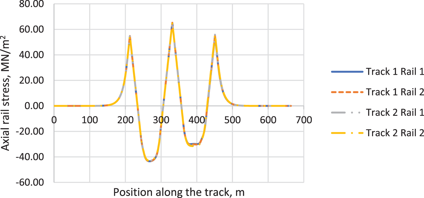
Axial rail stresses due to temperature differential –22.2°C applied to the superstructure.
Currently, there is no national code that would provide detailed guidance for rail break modeling and analysis. Similar to the RSI analysis in general, local agencies develop their codes based on their experience.
Stage construction analysis is used in this study to model the rail break and run the analysis. First, a temperature differential is applied to the model in increments. A rail member next to an expansion joint is then deconstructed (Fig. 9), and a progressive collapse analysis is performed. The progressive collapse analysis allows gradual redistribution of the released forces to the superstructure. The analysis employs adapting increments and arc-length control. An initial load factor of 0.01 is selected. The minimum and maximum load factors are 0.0001 and 1, correspondingly. Load factors are then automatically selected for each step to ensure analysis convergence. Figure 10 shows a relationship between the rail gap size and the load factor. An impact factor can be specified to account for the dynamic effects.
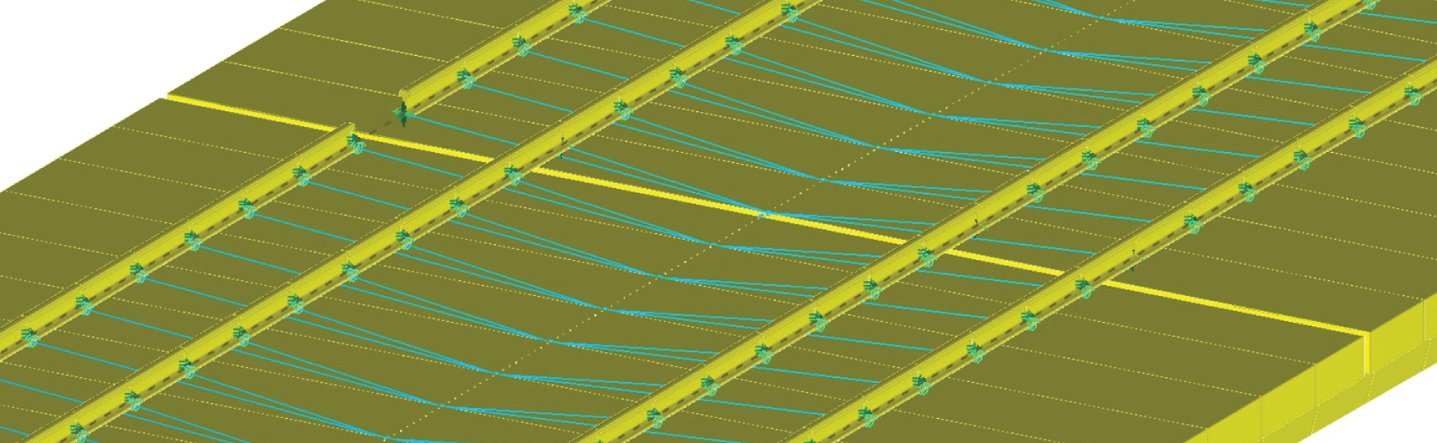
Rail break is simulated by deconstructing a rail member next to an expansion joint.
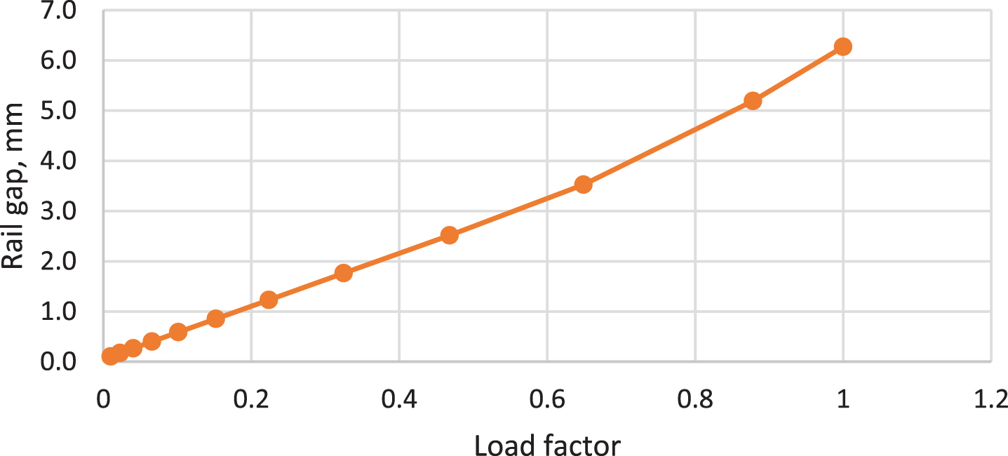
Rail gap after a thermal load of – 22.2°C is applied to the superstructure, and a break in Rail 2 of Track 2 is modeled. The relationship between rail gap and load factor.
The gap in the rail obtained through the collapse analysis is equal to 6.4 mm. Figure 11 shows the comparison of a static response obtained through the collapse analysis and a dynamic response obtained through nonlinear dynamic analysis. In order to perform a nonlinear dynamic analysis, fictitious zero loads are applied at the joints of a deconstructed member. These loads are assigned a fictitious variation in time with a zero magnitude. This approach allows running a nonlinear dynamic analysis without applying any additional loads and instead allows redistribution of forces from the deconstruction activity.
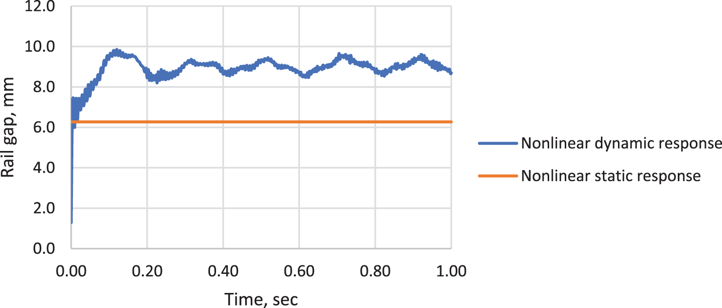
Rail gap after a thermal load of – 22.2°C is applied to the superstructure, and a break in Rail 2 of Track 2 is modeled.
The described method of modeling the rail break is easily implementable due to the use of the stage construction analysis capable of utilizing nonlinear elements.
Loading
Vehicle-track-structure-interaction (VTSI) analysis Level 1 (or Rolling Stock analysis) is a linear dynamic analysis that allows the dynamic application of a series of vertical vehicle loads. As opposed to the VTSI Level 2 analysis (see Section 5), the mass of the vehicle and its suspension system are not considered in this case.
In Sections 4 and 5, we use a train model adapted from Yang [10]. The detailed properties of the train are listed in Section 5. The total weight of the vehicle is the sum of the weights of the car (410 kN), two bogies (30 kN), and four wheelsets (17.5 kN), which is equal to 540 kN. This weight is distributed between the four wheelsets to form the load pattern shown in Fig. 12. The load is then distributed again between the two rails of the track.
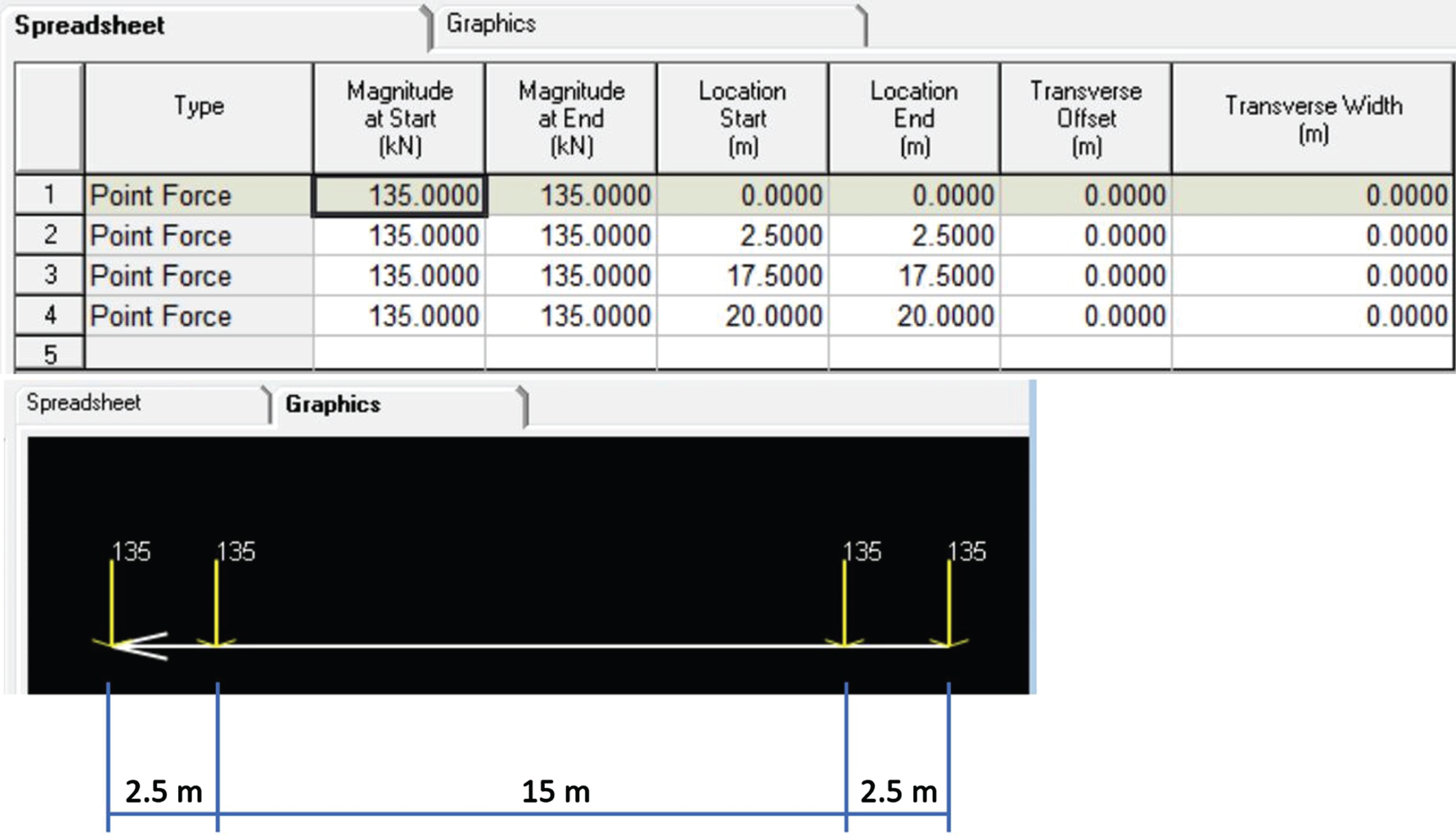
Load pattern for VTSI analysis Level 1.
One of the goals of dynamic VTSI analysis is to limit vertical deck accelerations. In order to evaluate deck accelerations under the vehicle traveling at various speeds, we utilize Stage Construction analysis to create 24 load steps. Each step contains a VTSI Level 1 load case with speeds varying from 40 to 110 m/sec as per TM 2.10.10 [3]. The maximum obtained accelerations are presented in Fig. 13. According to TM 2.10.10 [3], the maximum deck acceleration should be limited to 4.9 m/sec2. The obtained values are well below the limit for all the vehicle speeds.
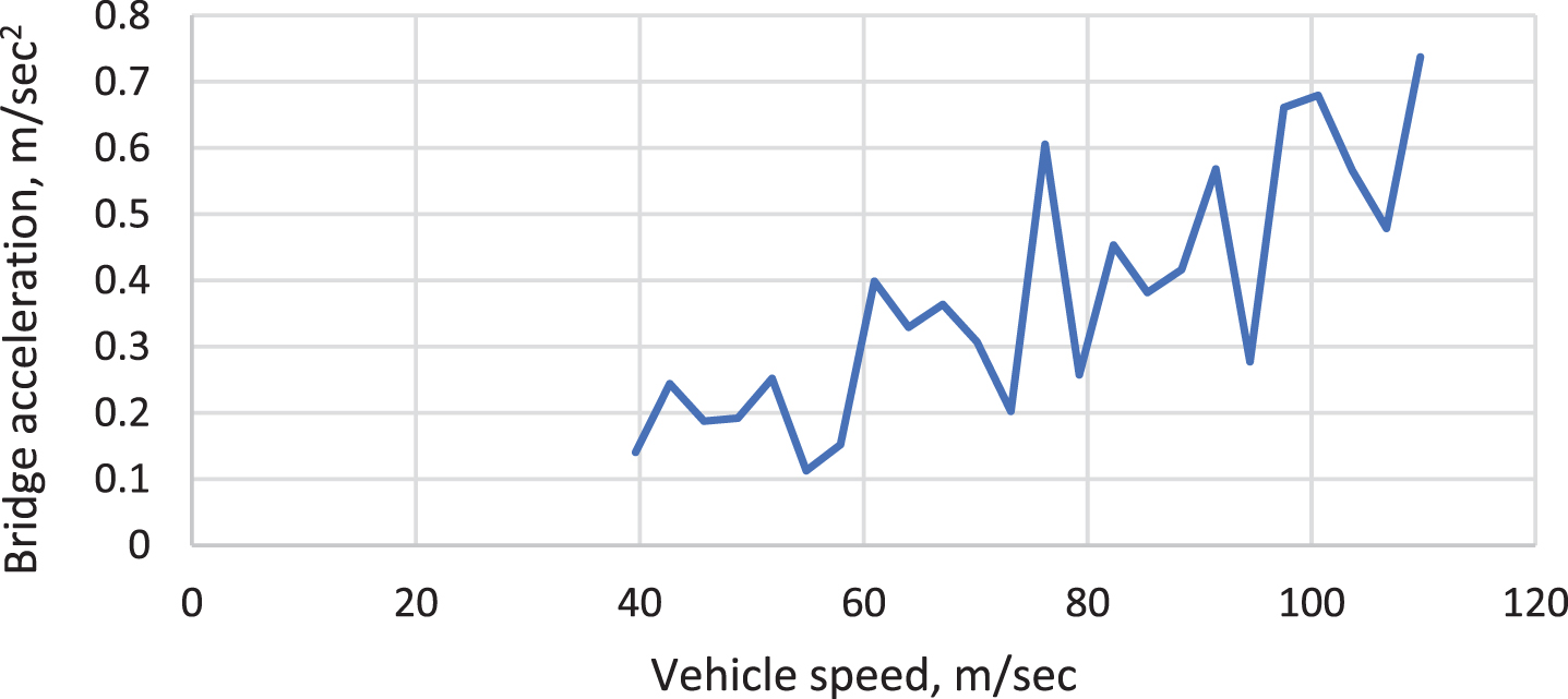
Peak vertical bridge acceleration in the middle of the second span with respect to vehicle speed.
Analysis methodology
The LARSA 4D VTSI analysis Level 2 is based on combining the three systems of equations of motion (for the vehicle, track, and structure) with constraint conditions. This approach has many advantages over the use of specialized VTSI software that models and analyzes the complete vehicle-structure system monolithically but may limit the types of structures that can be analyzed, or iterative procedures that solve the vehicle and structure systems separately, which may require significant computational resources since the convergence of the solution can be slow. For a detailed description of the analysis, see Fedorova and Sivaselvan [11].
For this analysis, the structure can be modeled using standard finite elements. Currently, the analysis is limited to straight bridges. The vehicle is modeled as a sequence of cars with user-defined properties. Each car is represented as a multibody system composed of rigid bodies, springs, and dashpots. The train and the track are coupled together using kinematic constraints.
Vehicle properties
The vehicle consists of a single car, two bogies, and four wheelsets (two per bogie), see Fig. 14. A wheelset consists of two rigidly connected wheels, one of which is positioned on the left rail and another on the right rail. The vehicle properties are as follows: car weight is 410 kN, mass moment of inertia of car body around the Y axis is entered as 2080 ton-m2, the longitudinal distance between two bogies is 17.5 m, the weight of the bogie is 30 kN, bogie mass moment of inertia around X and Y axes are 1.58 ton-m2 and 3.93 ton-m2, correspondingly, stiffness and damping of the secondary suspension are 265 kN/m and 45.1 kN-s/m, wheelset width is 1.5 m and equal to the gauge of the rails, wheel diameter is 0.91 m, wheelset weight is 17.5 kN, the longitudinal distance between two wheelsets is 2.5 m, wheelset mass moment of inertia around the X axis is 1.14 ton-m2, stiffness and damping of the primary suspension are 590 kN/m and 19.6 kN-s/m correspondingly.
Multibody vehicle model for VTSI analysis Level 2.
In this section, the results of VTSI analyses Level 1 and 2 are compared. The vehicle speed of 97.5 m/sec was chosen for the analysis.
The comparisons of bridge displacements and accelerations are presented in Figs. 15 and 16. It can be noted that the results of the two VTSI analyses match quite well. This can be explained by the fact that only one car per vehicle was modeled. With trains consisting of a larger number of cars, each passing car amplifies the response of the bridge, and the influence of car parts dynamics on the bridge response is expected to be more pronounced (see Section 6).
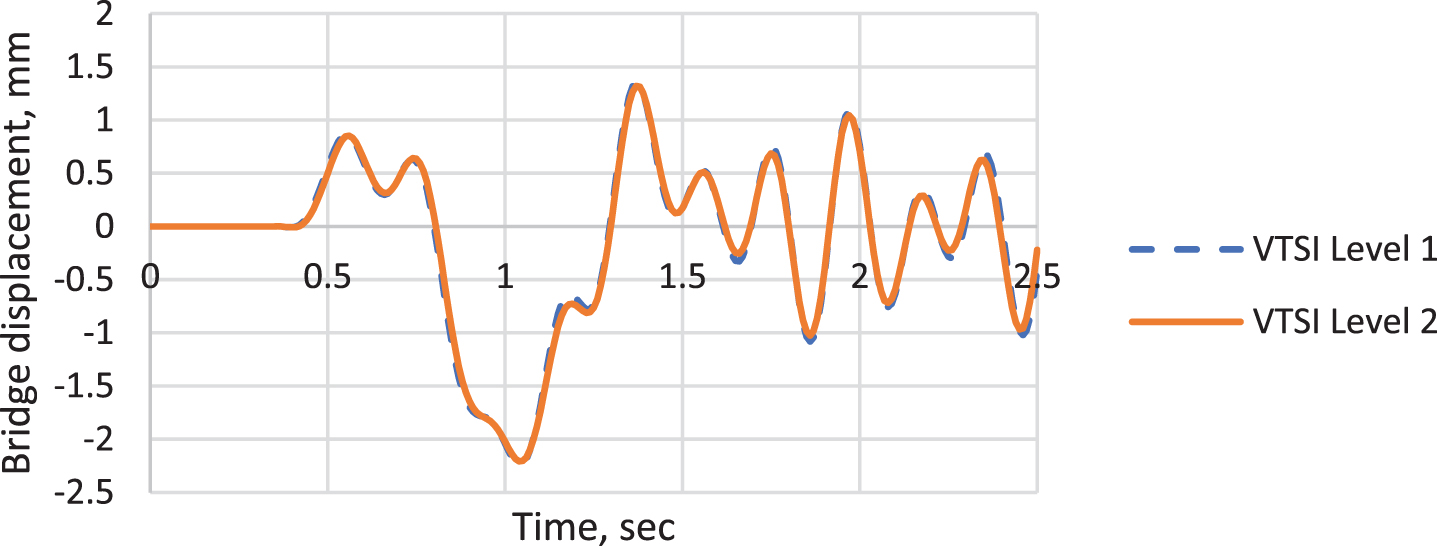
Vertical bridge displacement in the middle of the second span.
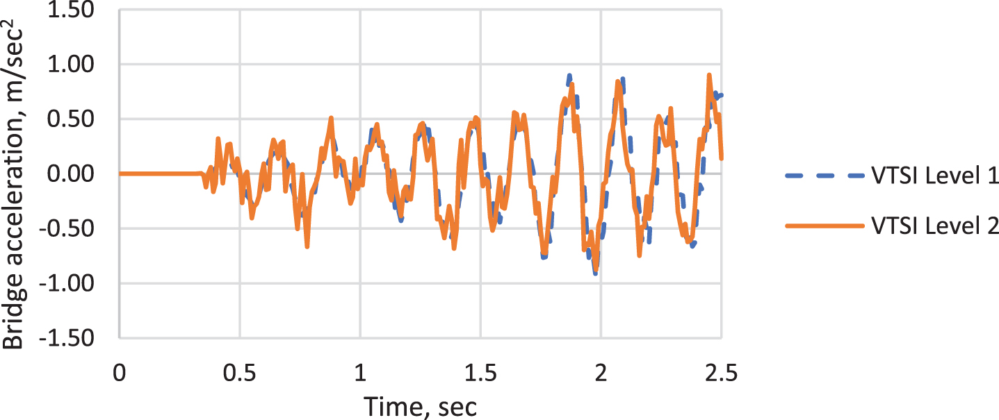
Vertical bridge acceleration in the middle of the second span.
Acceleration of the vehicle car body is obtained through the VTSI level 2 analysis and presented in Fig. 17. According to TM 2.10.10 [3], the maximum vertical acceleration within the car body is limited to 0.44 m/sec2. The obtained acceleration is well within this limit.
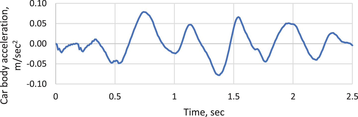
Vertical vehicle car body acceleration.
This section investigates the effect of train properties and speed variations on the bridge response.
Model description
The structure consists of a one-span simply supported straight bridge and track. The properties are listed in Section 2.3. The length of the span is 18 m. The first frequency of the bridge is 11.9 Hz.
Influence of vehicle speed on the impact factor
Impact factors obtained from code equations can be used to approximate a dynamic response of a structure when a static response is known. At the same time, impact factors can be calculated based on the results of a dynamic analysis with or without vehicle-structure interaction. For an example of a study on impact factors obtained from vehicle-structure interaction analysis, see Li [12]. Kimmle et al. [13] considered the effect of incorporating the train-structure interaction into the dynamic analysis of bridges under high-speed trains. One of the conclusions of that study is that accounting for the interaction allows, in some cases, for a significant reduction of the impact factors, compared to dynamic analysis without the train-structure interaction considered. As opposed to some known studies (Zeng [14], Frýba [15]), in this study, we include the track into the model while performing both types of analyses: with (VTSI Level 2) and without (VTSI Level 1) interaction.
In this subsection, a train is composed of 5 cars. Vehicle properties are listed in Section 5.2. First, we analytically determine the speeds at which the train moves in resonance with the structure. The phenomenon of resonance in structures under high-speed trains was extensively studied; for example, see Yang [10] and Li [16]. According to Yang [10], the resonant speed can be calculated as v res = f L/k, where f is the bridge frequency and L is the length of a car (k = 1, 2, 3, …). The first three resonant speeds can then be found as 297.4 m/s, 148.7, and 99.2 m/s.
In order to obtain the static response of the bridge, a moving load analysis was performed. This analysis utilizes the same series of loads as VTSI analysis Level 1 (see Fig. 12 for a load pattern of a single car). However, the dynamic effects are not considered. The deflection impact factor can then be calculated as (u dyn /u stat – 1), where u dyn is the maximum dynamic deflection in the middle of the span, obtained through either VTSI Level 1 or Level 2 analysis, u stat is the maximum static deflection at the same location, obtained through moving load analysis. We perform a series of analyses at train speeds ranging from 45 m/s to 106 m/s at 7.625 m/s intervals.
Figure 18 shows midspan bridge displacements obtained at a resonant speed of 99.2 m/s. It can be observed that the response of the bridge amplifies with each passing car. Figures 19 and 20 include the impact factor and maximum bridge displacements at the midspan, correspondingly. The resonant speed of 99.2 m/s can be observed. At this speed, VTSI Level 2 produces a higher impact factor than VTSI Level 1. However, at some other speeds, the response from VTSI analysis Level 1 is more significant. The following subsection shows that the impact factor is influenced by the number of cars.
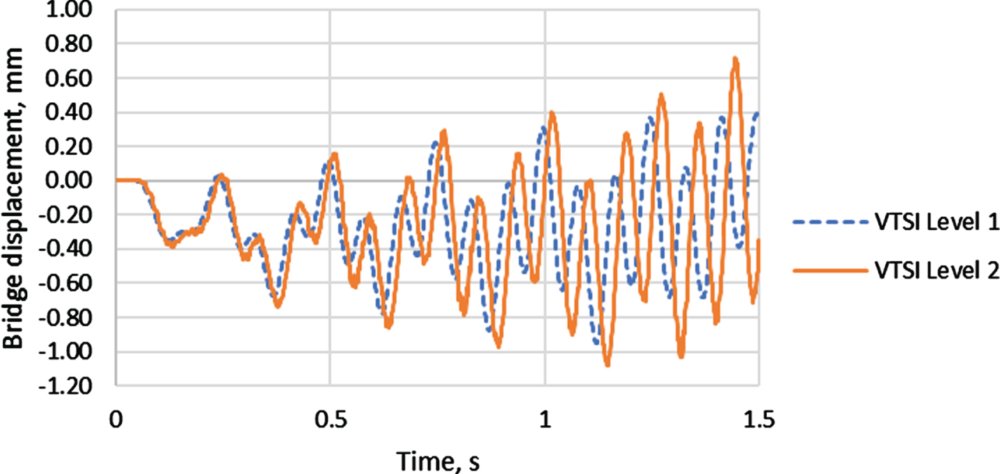
Vertical bridge displacements in the middle of the span.
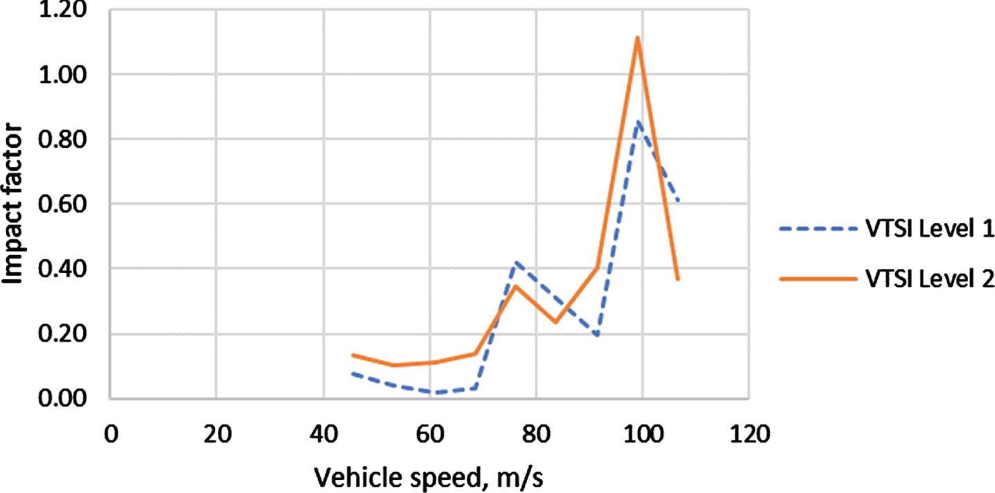
Deflection impact factors.
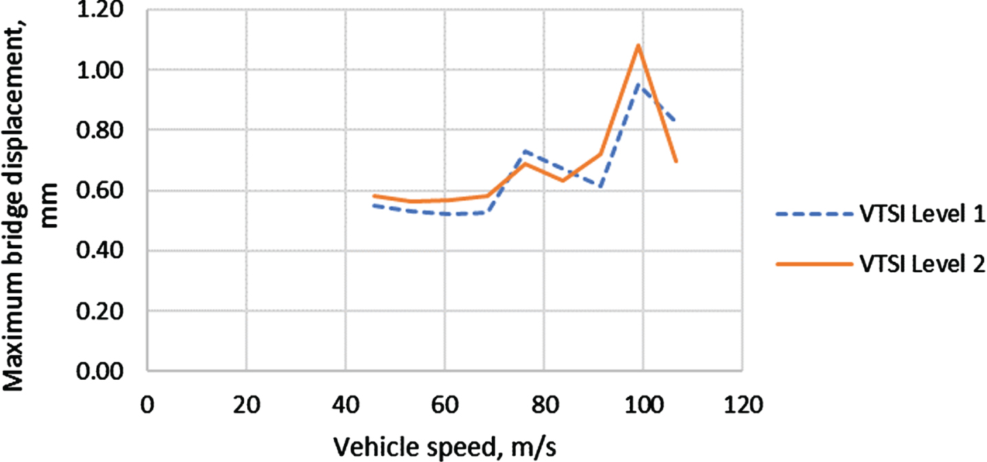
Maximum vertical bridge displacements in the middle of the span.
In this section, we consider four cases listed in Table 5. The cases present variations in train suspension parameters. While Case 1 contains realistic suspension properties (the same as in Section 5.2), Case 3 has artificially high suspension stiffness. Cases 2 and 4 correspond to Cases 1 and 3 but with damping values equal to zero. In this section, a single-car vehicle is used.
Four cases to study the effect of train suspension parameters on the impact factor
Four cases to study the effect of train suspension parameters on the impact factor
As expected, the lack of suspension damping produces higher impact factors. The stiffer suspension increases the impact factors as well. It can be noted that there is no well-defined resonant speed in Fig. 21, since only one car crosses the bridge.
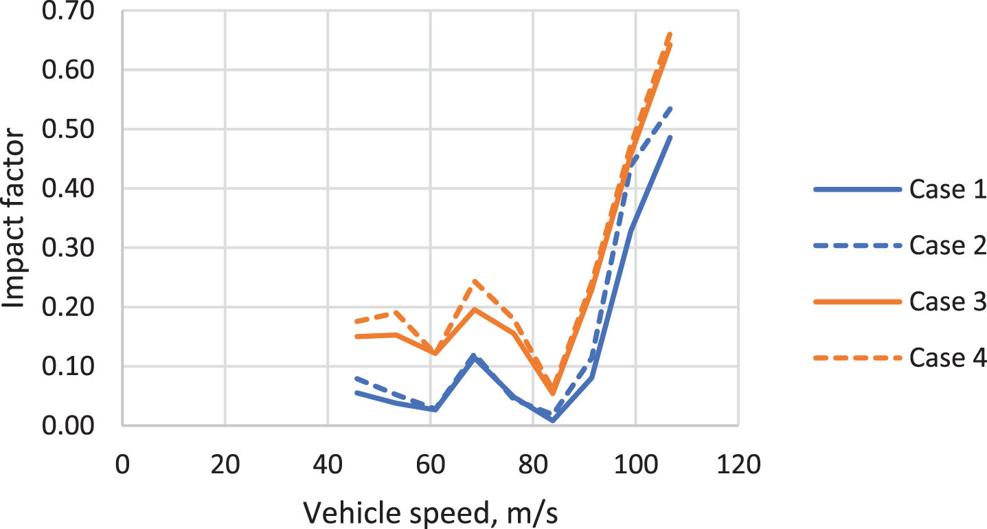
Influence of train parameters on the deflection impact factor.
Ultimately, as can be seen from this subsection and the previous one, the impact factor varies with the number of cars and train parameters.
In this paper, we have given an overview of two analysis types (RSI and VTSI) required in the design of railroad structures. The generation of a track-structure model was described in detail, as well as the ways to expedite the model generation. RSI analysis of an example structure was performed under vertical, longitudinal, and thermal loads. The results were compared to limit values provided by the technical memorandum CHSTP TM 2.10.10 [3]. The applications of two analysis types to simulate a rail break were then discussed. The stage construction analysis capable of incorporating inelastic elements was utilized. A part of the rail was deconstructed, followed by a progressive collapse or nonlinear time history analysis. While no national design code provides detailed guidance on performing this type of analysis, the described approach allows for straightforward modeling and analysis of the rail break using a standard RSI model. The following sections presented examples of VTSI analyses Level 1 and 2. VTSI analysis Level 1 includes a series of moving loads and may be sufficient if a structure under consideration meets code requirements and the response of vehicle components is not required. On the other hand, if a critical structure cannot meet track serviceability, RSI, or VTSI requirements outlined in TM 2.10.10 [3], the VTSI analysis Level 2 is required. Specifically, if the limit values of vertical displacements, rail stresses, and bridge accelerations given in Sections 3.3 and 4.2 are exceeded. In this case, the vehicle model should be considered a multibody system with wheels, bogies, car bodies, and suspensions. It was shown that when only a single train car was considered, the results obtained from the two analyses were comparable. However, once a larger number of cars was introduced, the differences in the bridge response were observed. For example, for the studied structure, the impact factor obtained from VTSI analysis Level 2 was higher than from Level 1 when the vehicle moved at a resonant speed. The effects of variations in train parameters and speed on the bridge response were studied by introducing four study cases with various primary and secondary suspension parameters. It was shown that the impact factors were affected by the choice of train parameters. This observation reinforces the conclusion that standard impact factors obtained from design codes might not accurately represent dynamic impacts from trains passing at high speeds.