On characterizations of randomized computation using plain Kolmogorov complexity 1

Abstract

Allender, Friedman, and Gasarch recently proved an upper bound of $PSPACE$ for the class ${DTTR}_{K}$ of decidable languages that are polynomial-time truth-table reducible to the set of prefix-free Kolmogorov-random strings regardless of the universal machine used in the definition of Kolmogorov complexity. It is conjectured that ${DTTR}_{K}$ in fact lies closer to $BPP$ , a lower bound established earlier by Buhrman, Fortnow, Koucký, and Loff. It is also conjectured that we have similar bounds for the analogous class ${DTTR}_{C}$ defined by plain Kolmogorov randomness. In this paper, we provide further evidence for these conjectures. First, we show that the time-bounded analogue of ${DTTR}_{C}$ sits between $BPP$ and $PSPACE \cap P / poly$ . Next, we show that the class ${DTTR}_{C, α}$ obtained from ${DTTR}_{C}$ by imposing a super-constant minimum query length restriction on the reduction lies between $BPP$ and $PSPACE$ . Finally, we show that the class $P / R_{C^{t}}^{= log}$ obtained by further restricting the reduction to ask queries of logarithmic length lies between $BPP$ and $Σ_{2}^{p} \cap P / poly$ .

Keywords

Kolmogorov complexity randomness truth-table reductions

1. Introduction

The word “randomness” is used in at least two different contexts in computation theory: One is in the theory of Kolmogorov complexity, which measures randomness of a finite string in terms of incompressibility. The other randomness refers to coin flips used for efficient computation, and gives rise to (among others) the complexity class $BPP$ . Despite the remote origins of these two notions of randomness, some interesting links between them have been found in recent work by Allender et al. [2–5]: they conjectured, and gave some evidence, that $BPP$ is characterized as the class of languages truth-table reducible to the set of Kolmogorov random strings, that is, those decidable in deterministic polynomial time by asking the oracle non-adaptively whether a string is random. Our aim is to strengthen this connection between Kolmogorov randomness and $BPP$ .

Let $C_{U} (x)$ denote the Kolmogorov complexity of a string $x \in {0, 1}^{*}$ , i.e., the length of the shortest description of x when a fixed universal machine U is used as a decoder (see Section 2.1). Depending on whether or not the machine is required to be prefix-free, this complexity is called the prefix-free or plain complexity, and for the former it is customary to write $K_{U}$ instead of $C_{U}$ . We consider the set $R_{C_{U}}$ (or $R_{K_{U}}$ ) of random strings, i.e., those that have no description shorter than themselves: $R_{f} = {x \in {0, 1}^{*} ∣ f (x) ⩾ | x |}$ .

Buhrman, Fortnow, Koucký, and Loff [7] showed that every language in $BPP$ reduces to the set of random strings via polynomial-time truth-table reducibility (denoted $⩽_{tt}^{p}$ in the following theorem, see Definition 2.1), regardless of whether the machine defining the random strings is plain universal or prefix-free universal:

Theorem 1.1 ([7]).

For every language $L \in BPP$ , we have $L ⩽_{tt}^{p} R_{C_{U}}$ for any universal machine U, and $L ⩽_{tt}^{p} R_{K_{U}}$ for any prefix-free universal machine U.

Theorem 1.1 gives a lower bound of $BPP$ for the class of languages that reduce to $R_{C_{U}}$ or $R_{K_{U}}$ , but this bound is obviously not “tight,” as the sets $R_{C_{U}}$ and $R_{K_{U}}$ are undecidable [10]. However, we obtain an interesting upper bound if we take the intersection over all universal machines U. That is, let ${DTTR}_{K}$ be the class of languages L such that $L ⩽_{tt}^{p} R_{K_{U}}$ for all universal prefix-free machines U. Surprisingly, Cai, Downey, Epstein, Lempp and Miller [8] showed that every language in ${DTTR}_{K}$ is decidable, and moreover Allender, Friedman, and Gasarch [5] showed:

Theorem 1.2 ([5]).

${DTTR}_{K} \subseteq PSPACE$ .

Combining Theorems 1.1 and 1.2, we have $BPP \subseteq {DTTR}_{K} \subseteq PSPACE$ . The question then arises: to which does ${DTTR}_{K}$ sit closer, $BPP$ or $PSPACE$ ? Allender [1] has conjectured the following:

Conjecture 1.3 ([1]).

$BPP = {DTTR}_{K}$ .

The conjecture is more plausible when we consider time-bounded prefix-free Kolmogorov complexity. Allender, Buhrman, Friedman, and Loff [2] defined the classes called ${TTRT}_{K}$ and ${TTRT}_{K}^{'}$ , which are time-bounded versions of ${DTTR}_{K}$ , and showed the following (“ $/ α$ ” means advice strings of length α [6, Definition 6.16]):

Theorem 1.4 ([2]).

$BPP \subseteq {TTRT}_{K} \subseteq PSPACE / α \cap P / poly$ for any nondecreasing unbounded computable function $α : N \to N$ .

$BPP \subseteq {TTRT}_{K}^{'} \subseteq PSPACE \cap P / poly$ .

Less is known about the analogous classes ${DTTR}_{C}$ , ${TTRT}_{C}$ , ${TTRT}_{C}^{'}$ for plain Kolmogorov complexity (see Definitions 4.4 and 3.1). We know that these classes all contain $BPP$ by Theorem 1.1 or by a similar argument. For the upper bound, Allender et al. [5] conjecture that ${DTTR}_{C} \subseteq PSPACE$ (similarly to Theorem 1.2), but in reality we do not even know whether ${DTTR}_{C}$ equals all decidable languages. The techniques used by Allender et al. [2,5] to prove Theorems 1.2 and 1.4 make use of the coding theorem and thus cannot be directly applied to $C_{U}$ (see the discussion in [5, Section 5]).

In Section 3, we prove the same inclusions for ${TTRT}_{C}$ and ${TTRT}_{C}^{'}$ as Theorem 1.4 states for prefix-free complexity.

In Section 4, we consider a weaker reduction $⩽_{{tt}_{α}}^{p}$ (see Definition 4.1) in which we cannot query a string of length less than $α (n)$ , where n is the input length. We prove that for the corresponding classes ${TTRT}_{C, α}$ and ${DTTR}_{C, α}$ , the upper bound can be improved to $PSPACE$ (while the $BPP$ lower bound remains true).

In Section 5, we restrict the reduction further, allowing only queries of exactly logarithmic length. This defines the subclass $P / R_{C^{t}}^{= log} \subseteq {TTRT}_{C, log}$ , which still contains $BPP$ . We prove that $P / R_{C^{t}}^{= log} \subseteq Σ_{2}^{p} \cap P / poly$ . The upper bound of $Σ_{2}^{p}$ comes from a 1-round game played between two players. Together with the $BPP$ lower bound, this gives an alternative explanation of the well-known inclusion $BPP \subseteq Σ_{2}^{p}$ .

In view of this upper bound of $Σ_{2}^{p} \cap P / poly$ , we believe that the following characterization of $BPP$ is quite likely, and propose this as a step towards Conjecture 1.3.

Conjecture 1.5.
$BPP = P / R_{C^{t}}^{= log}$ .

2. Preliminaries and notations

We regard the set of strings ${0, 1}^{*}$ as equipped with the length-increasing lexicographical order. For a set of strings $A \subseteq {0, 1}^{*}$ and a natural number $n \in N$ , $A^{= n}$ , $A^{⩽ n}$ , and $A^{< n}$ are defined as $A \cap {0, 1}^{n}$ , $⋃_{m ⩽ n} A^{= m}$ , and $⋃_{m < n} A^{= m}$ , respectively. We abbreviate ${({0, 1}^{*})}^{⩽ n}$ as ${0, 1}^{⩽ n}$ . For a set A, $\overline{A}$ denotes the complement of A.

For functions $s, t : N \to N$ , we write $s ⩽ t$ if $s (n) ⩽ t (n)$ for all $n \in N$ . A nondecreasing and time-constructible function $t : N \to N$ is called a time bound. For a nondecreasing and unbounded function $t : N \to N$ , define $t^{- 1}$ as $t^{- 1} (n) = min {m \in N ∣ t (m) > n}$ . Then ${(t^{- 1})}^{- 1} ⩽ t$ holds because ${(t^{- 1})}^{- 1} (n) = min {m ∣ t^{- 1} (m) > n}$ and $t^{- 1} (t (n)) = min {m ∣ t (m) > t (n)} > n$ .

We assume that the reader is familiar with basics of complexity theory [6].

In this paper, we mainly discuss truth-table (i.e., non-adaptive) reductions to the set of random strings.

Definition 2.1.
For languages $A, B \subseteq {0, 1}^{*}$ , we write $A ⩽_{tt}^{p} B$ if there exists a polynomial time Turing machine M that, on input x, outputs an encoding of a circuit λ and a list of queries $q_{1}, \dots, q_{m}$ so that $A (x) = λ (B (q_{1}), \dots, B (q_{m}))$ .

2.1. Kolmogorov complexity

We review some basic definitions and facts about Kolmogorov complexity. For details, see Li and Vitányi [10].

The Kolmogorov complexity of a string x on a Turing machine U is defined as the length $C_{U} (x) = min {| d | ∣ U (d) = x} \in N \cup {\infty}$ of the shortest description d of x when using U as a decoder. We also consider the time-bounded version: for a time bound t, we write $C_{U}^{t} (x)$ for the length of the shortest input d that causes U to outputs x in at most $t (| x |)$ time steps (note that time is measured in terms of the output length).

As mentioned at the beginning, it is sometimes required that the domain of U is prefix-free, i.e., if $U (d)$ is defined, then $U (d^{'})$ is undefined for any proper prefix $d^{'}$ of d. In this case, it is customary to write $K_{U}$ instead of $C_{U}$ (and call it prefix-free complexity).

We will be interested in the set $R_{f} = {x \in {0, 1}^{*} ∣ f (x) ⩾ | x |}$ of random (or incompressible) strings where $f = C_{U}$ , $C_{U}^{t}$ , etc.

Of course, Kolmogorov complexity, and hence the set of random strings, depend on U. It is therefore important to use the “best” machine U in the following sense:

Definition 2.2.
A Turing machine U is said to be universal if for each Turing machine M, there exists $c_{M}$ such that for any $x \in {0, 1}^{}$ , $C_{U} (x) ⩽ C_{M} (x) + c_{M}$ .

It is known that there exists a Turing machine U which simulates every Turing machine M (see [6]), and it is not hard to see that U is universal. Thus, we usually fix one such machine U and discuss complexity with respect to it.

For prefix-free Kolmogorov complexity, the Turing machines U and M in Definition 2.2 are required to be a prefix-free machine.

For time-bounded Kolmogorov complexity, some slowdown is needed when a universal Turing machine U simulates each machine M. Therefore, we introduce a parameter $f : N \to N$ , which means that U must simulate M within $f (s)$ steps if M halts within s steps. This is the notion of f-efficient universality*:
Definition 2.3 ([2]).

For a time bound $f : N \to N$ , a Turing machine U is said to be f-efficient universal if U is universal, and there exists a constant $c_{M}$ for each Turing machine M, such that for any time bounds t and $t^{'}$ , for all but finitely many x, $t (| x |) ⩾ f (t^{'} (| x |))$ implies $C_{U}^{t} (x) ⩽ C_{M}^{t^{'}} (x) + c_{M}$ . We say that U is time-efficient universal if it is p-efficient universal for some polynomial p.

Time-efficient universality means that the machine U is allowed to simulate each machine with a polynomial slowdown.

3. Bounds for time-bounded Kolmogorov complexity

Our goal for this section is to prove an analogue of Theorem 1.4 for plain Kolmogorov complexity. First, let us define the classes ${TTRT}_{C}$ and ${TTRT}_{C}^{'}$ by using time-efficient universality and f-efficient universality, respectively.

Definition 3.1 ([2]).

${TTRT}_{C}$ contains all the languages L such that for all sufficiently large t and for any time-efficient universal Turing machine U, $L ⩽_{tt}^{p} R_{C_{U}^{t}}$ . In short, ${TTRT}_{C} = {L \subseteq {0, 1}^{*} ∣ \exists t_{0}, \forall t ⩾ t_{0}, \forall U, L ⩽_{tt}^{p} R_{C_{U}^{t}}}$ .

${TTRT}_{C}^{'}$ contains all the languages L such that for each computable function f, there exists $t_{0}$ such that for all $t ⩾ t_{0}$ and any f-efficient universal Turing machine U, $L ⩽_{tt}^{p} R_{C_{U}^{t}}$ .

It is easy to see that ${TTRT}_{C}^{'} \subseteq {TTRT}_{C}$ by letting $f (n) = 2^{n}$ . It should be noted that the motivation of [2] for allowing such a slow prefix-free universal machine comes from the fact that it is not clear how to define time-efficient coding schemes for prefix-free Kolmogorov complexity (see [2, Section 5]). Here we adapted their definitions to the case of plain Kolmogorov complexity, and show the following:

Theorem 3.2.

$BPP \subseteq {TTRT}_{C} \subseteq PSPACE / α \cap P / poly$ for any nondecreasing unbounded computable function $α : N \to N$ .

$BPP \subseteq {TTRT}_{C}^{'} \subseteq PSPACE \cap P / poly$ .

Proof of Part 1 of Theorem 3.2.
We have $BPP \subseteq {TTRT}_{C}^{'} \subseteq {TTRT}_{C} \subseteq P / poly$ because this was proved in [2,7] regardless of whether the Kolmogorov complexity defining the classes is plain or prefix-free. All we have to show is that ${TTRT}_{C} \subseteq PSPACE / α$ .

For simplicity, we show that ${TTRT}_{C} \subseteq PSPACE / 2^{α}$ for any function α that satisfies the stated property. Assume, by way of contradiction, that $L \in {TTRT}_{C} ∖ PSPACE / 2^{α}$ . Then $L ⩽_{tt}^{p} R_{C_{U}^{t_{0}}}$ holds for some time bound $t_{0}$ and some Turing machine U. Since $R_{C_{U}^{t_{0}}}$ is decidable, L is also decidable. Let $t_{L}$ denote a time bound such that it is decidable whether $x \in L$ or not in time $t_{L} (| x |)$ .

Given any time bound $t_{0}$ , we will show that there exist a time-efficient universal Turing machine U and a time bound $t^{} ⩾ t_{0}$ such that $L ≰_{tt}^{p} R_{C_{U}^{t^{}}}$ . This means that $L \notin {TTRT}_{C}$ , which contradicts the assumption. In order to show it, a time-efficient universal Turing machine U is constructed by combining two Turing machines, $U_{0}$ and M. The following lemma states that if $U_{0}$ is time-efficient universal, then U is. Lemma 3.3.
Let $U_{0}$ be a time-efficient universal Turing machine. Suppose that for a time bound t, M is a Turing machine such that, for all but finitely many x, M either halts in $t {(| x |)}^{2}$ steps or does not halt. Then there exists a Turing machine U such that for some $t^{} = Θ (t^{2})$ , $C_{U}^{t^{}} (x) = min {C_{U_{0}}^{t} (x) + 2, C_{M}^{t^{2}} (x) + 1}$ for all large $| x |$ . Moreover, U is again a time-efficient universal Turing machine.
Proof.
Define U as follows: On input $00 d$ , U runs $U_{0}$ on input d. Suppose that $U_{0}$ outputs x after s steps. Then U outputs x after it waits $s^{2}$ steps. On input $1 d$ , U outputs $M (d)$ . Otherwise U does not halt. Note that the steps to calculate $U_{0} (d)$ can be counted by adding some tapes to U.

Let $p (s)$ be the number of steps2
²
One may think of p as $p (s) = s^{2}$ by carefully constructing U so that U halts in exactly $s^{2}$ steps when $U_{0}$ halts in s steps. Here we avoided such a technical argument that depends on computational models.

it takes for U to halt on input $00 d$ , where s denotes the number of steps to calculate $U_{0} (d)$ . Note that $p (s)$ includes the steps it takes to run $U_{0}$ , to compute $s^{2}$ , and so on. We can assume that $p (s) ⩾ s^{2}$ and $p (s)$ does not depend on d, and that $t^{} (n) : = p (t (n)) = Θ (t {(n)}^{2})$ is again a time bound.

Then $U (00 d) = x$ in at most $t^{} (| x |)$ steps if and only if $U_{0} (d) = x$ in at most $t (| x |)$ steps for any time bound t. One can verify that the lemma follows by this property. □

Fix a standard time-efficient universal Turing machine $U_{0}$ for reference. A Turing machine M will be defined later. Let U be the time-efficient universal machine defined in Lemma 3.3 for some time bound t fixed later in Claim 2. In order to derive a contradiction, M is constructed by a diagonalization argument so that it fools each Turing machine that computes a truth-table reduction $⩽_{tt}^{p}$ . It should be noted that, in Lemma 3.3, M is allowed to run in $t^{2}$ steps whereas $U_{0}$ runs in at most t steps; hence, the output of M can be defined depending on the output of $U_{0}$ for a fixed output length. In the course of computation of M, M holds an approximation of $R_{C_{U}^{t^{}}}$ denoted by R. More precisely, R is first set to be ${0, 1}^{}$ , always $R \supseteq R_{C_{U}^{t^{}}}$ holds, and $max {k \in N ∣ R^{< k} = R_{C_{U}^{t^{}}}^{< k}}$ increases as calculation proceeds. Since $\overline{R}$ is finite, we can store it. Note that, by the property of Lemma 3.3, $R_{C_{U}^{t^{}}} = R_{C_{U_{0}}^{t} + 2} \cap R_{C_{M}^{t^{2}} + 1}$ except for finitely many strings.

Let us efficiently enumerate all polynomial-time Turing machines that compute polynomial-time truth-table reductions, namely $γ_{1}, γ_{2}, \dots$ . This can be done by putting a clock of $n^{e} + e$ on $γ_{e}$ and by regarding the output of $γ_{e} (x)$ as a circuit $λ_{e, x}$ and queries $q_{1}, \dots, q_{k}$ (see Definition 2.1). Since $U_{0}$ is out of our control, we will play a game against $U_{0}$ in order to make the output of the circuit $λ_{e, x}$ differ from $L (x)$ . As we will show, we can always do so for some x; otherwise L is equal to a winning side, and thus $L \in PSPACE$ , which contradicts the assumption. This idea is originally due to Allender et al. [5]. Now let us precisely define the game $G_{e, x}$ for some $γ_{e}$ and some x.

Description of the game.* The game $G_{e, x}$ is played between two players, the YES player and the NO player. At the start of the game, randomness of the strings of length less than $α (| x |)$ is fixed and each player does not disturb $R^{< α (| x |)}$ anymore. (More formally, compute $R_{C_{U_{0}}^{t} + 2}^{< α (| x |)}$ and let $R : = R \cap R_{C_{U_{0}}^{t} + 2}^{< α (| x |)}$ .) During the game, R is going to be altered by moves of the players. The current value of the game, denoted by $val (R)$ , is defined as $λ_{e, x} (R (q_{1}), \dots, R (q_{k}))$ . Note that $val (R)$ is equal to the value of $γ_{e} (x)$ regarded as a truth-table reduction to R.

Let $l : = max {l, | q_{1} |, \dots, | q_{k} |}$ , where l denotes a variable of the algorithm of M. The game has rounds from $α (| x |)$ to l. In the rth round, where $α (| x |) ⩽ r ⩽ l$ , the YES player first decides $Z_{1} \subseteq {0, 1}^{r}$ such that $| Z_{1} | ⩽ 2^{r - 2}$ . This means that the YES player declares that each element of $Z_{1}$ is not random. Next, the NO player decides $Z_{0} \subseteq {0, 1}^{r}$ such that $| Z_{0} | ⩽ 2^{r - 2}$ . Then let $R : = R ∖ (Z_{0} \cup Z_{1})$ at the end of the round. After all the rounds end, the YES player wins if $val (R) = 1$ and the NO player wins otherwise. Since the game is finite and deterministic, exactly one of the players has a winning strategy. Let ${WIN}_{e, x} \in {0, 1}$ denote which player is going to win the game $G_{e, x}$ .

The ${WIN}_{e, x}$ side plays the game optimally according to a winning strategy against $U_{0}$ . Suppose that the player of the ${WIN}_{e, x}$ side chooses $Z \subseteq {0, 1}^{r}$ in the rth round and $| d | = r - 2$ , where d is the input of M. Let $Z = {z_{1} < z_{2} < \dots < z_{k}}$ , where $k ⩽ 2^{r - 2}$ . If, for $i ⩽ k$ , the input d is the ith string in ${0, 1}^{r - 2}$ in the lexicographical order, then M outputs $z_{i}$ and halts. This makes $z_{i}$ not random since $M (d) = z_{i}$ and $| d | < | z_{i} | - 1$ . If not, M does not halt, and continues computation.

On the other hand, $U_{0}$ plays the role of the opponent of the ${WIN}_{e, x}$ side. The opponent always moves $Z = {(\overline{R_{C_{U_{0}}^{t} + 2}})}^{= r}$ in the rth round. Note that $| Z | = | {(\overline{R_{C_{U_{0}}^{t} + 2}})}^{= r} | ⩽ 2^{r - 2}$ holds (see [10, Definition 2.2.1 and Theorem 2.2.1]).

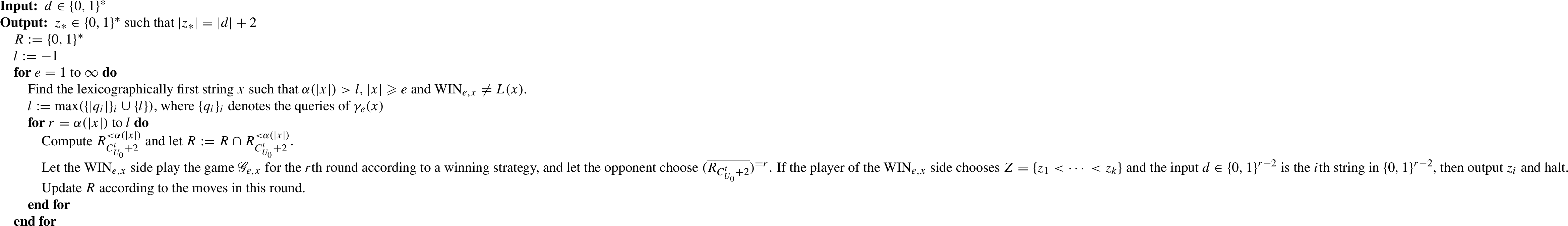
The overall algorithm of M is shown in Algorithm 1. Note that what M outputs is determined by a move of the player who has a winning strategy.

Algorithm 1
Algorithm of M

Analysis. Let us move on to analysis of the algorithm. We first claim that there always exists a “witness” $x \in {0, 1}^{}$ such that ${WIN}_{e, x} \neq L (x)$ . Claim 1.
M can always find a string x such that* $α (| x |) > l$ and ${WIN}_{e, x} \neq L (x)$ .
Proof.
Suppose that M fails to find such a string x at some point, which implies that ${WIN}_{e, x} = L (x)$ for all x with $| x | ⩾ α^{- 1} (l)$ . We present an algorithm to decide the language ${WIN}_{e, } = {x \in {0, 1}^{} ∣ {WIN}_{e, x} = 1}$ in $PSPACE / 2^{α}$ . On input x, let the advice give the truth-table of $R_{C_{U_{0}}^{t} + 2}^{< α (| x |)}$ . This can be encoded with $2^{α (| x |)} - 1$ bits. We know the value $α (| x |)$ by the length of the advice. Thus, this advice enables us to construct the game $G_{e, x}$ . Then the winning side, ${WIN}_{e, x}$ , can be computed by the standard minimax algorithm. Note that there exist at most exponentially many moves since a move Z is meaningful only if $Z \subseteq {q_{1}, \dots, q_{k}}$ , where k is bounded by a polynomial in $| x |$ .

Since ${WIN}_{e, x} = L (x)$ for all sufficiently large x, we can conclude that $L \in PSPACE / 2^{α}$ . This, however, contradicts the assumption. □

Next, we fix a fast-growing time bound t so that M halts within $t^{2}$ steps. Claim 2.
There exists a time bound t such that M halts within $t {(| z |)}^{2}$ steps for all large $| z |$ if M outputs z.
Proof.
Suppose that M halts at the rth round of the game $G_{e, x}$ . Note that $| d | + 2 = | z | = r ⩾ α (| x |)$ . M has computed $R_{C_{U_{0}}^{t} + 2}^{⩽ r}$ so far. It takes $O (\sum_{r^{'} ⩽ r} t (r^{'}) 2^{r^{'}})$ time steps. M has also calculated ${WIN}_{e, y}$ and $L (y)$ for each $y ⩽ x$ . It takes $2^{| x |^{O (e)}} + O (2^{| x | + 1} t_{L} (| x |)) ⩽ 2^{| x |^{O (| x |)}} t_{L} (| x |)$ time since we chose x so that $| x | ⩾ e$ in Algorithm 1. M needs to compute $α (m)$ for each $m ⩽ | x |$ . Let $t_{α} (m)$ denote the number of steps to compute $α (m)$ .

The length of x is bounded by $α^{- 1} (r)$ since $α (| x |) ⩽ r$ . Then the number of overall time steps is roughly less than $\begin{matrix} (1) & 2^{α^{- 1} {(r)}^{O (α^{- 1} (r))}} t_{L} (α^{- 1} (r)) + \sum_{0 ⩽ r^{'} ⩽ r} t (r^{'}) 2^{r^{'}} + \sum_{0 ⩽ m ⩽ α^{- 1} (r)} t_{α} (m) . \end{matrix}$ The second term is linear in $t (r)$ , and the other terms do not depend on t. Thus t can be defined as a sufficiently fast growing function $⩾ t_{0}$ so that (1) is less than $t {(r)}^{2}$ for all large r. □

Claim 2 ensures that R converges to $R_{C_{U}^{t^{}}}$ as time passes. Finally, we claim that each Turing machine is indeed fooled. Claim 3.
$L ≰_{tt}^{p} R_{C_{U}^{t^{}}}$ .
Proof.
After the game $G_{e, x}$ has been played out, since the ${WIN}_{e, x}$ side wins, $val (R) = {WIN}_{e, x} \neq L (x)$ holds at this point. Let $l_{e}$ denote the value of l in the eth outer loop before the inner loop in Algorithm 1. Then, in the later game $G_{e^{'}, x^{'}}$ for $e^{'} > e$ , we have $| q_{i} | ⩽ l_{e} ⩽ l_{e^{'}} < α (| x^{'} |)$ , which implies that the later computation does not disturb the value $R (q_{i})$ . Therefore, $R^{⩽ l}$ is actually equal to $R_{C_{U}^{t^{}}}^{⩽ l}$ after $G_{e, x}$ ends. It follows that $γ_{e}$ does not compute a truth-table reduction to $R_{C_{U}^{t^{}}}$ since the answer of the truth-table reduction on input x is equal to $val (R)$ , which is not equal to $L (x)$ . □

Claim 3 contradicts the assumption that $L \in {TTRT}_{C}$ . □

Let us review why the slight nonuniformity α is needed: To determine a time bound to calculate M, $| x |$ is bounded by the inequality $α (| x |) ⩽ r$ in Claim 2. The inequality is derived from fixing randomness of strings whose length is less than $α (| x |)$ . If α is slow enough, then the initial segment $R_{C_{U_{0}}^{t} + 2}^{< α (| x |)}$ is decidable in $PSPACE$ . However, since the definition of ${TTRT}_{C}$ uses time-efficient universality, M must run in at most polynomial time in t. This time limit prevents α from growing slowly because $| x |$ becomes huge as α becomes slow.

In the case of ${TTRT}_{C}^{'}$ , since a f-efficient universal Turing machine U is allowed to run longer than a time-efficient one, the Turing machine M can also run long enough to calculate the initial segment $R_{C_{U_{0}}^{t} + 2}^{< α (| x |)}$ . Therefore, we can eliminate the slight nonuniformity as stated in Part 2 of Theorem 3.2.
Proof of Part 2 of Theorem 3.2.
The proof is similar to that of Theorem 3.2.1. We prove only the inclusion ${TTRT}_{C}^{'} \subseteq PSPACE$ .

Suppose that $L \in {TTRT}_{C}^{'} ∖ PSPACE$ . Let $t_{L}$ be a time bound to compute L, and let h be a fast growing time bound such that for any constant d and for all large n, $2^{n^{d}} t_{L} (n) ⩽ h (n)$ .

Fix a p-efficient universal Turing machine $U_{0}$ for some time bound p. For a time bound t, let $α = t^{- 1}$ . We construct M in exactly the same way with the proof of Theorem 3.2.1, using $U_{0}$ , t and α. Let r denote the length of output of M. The running time of M is bounded by $2^{t {(r)}^{O (1)}} t_{L} (t (r))$ because the second and third terms of (1) in the proof of Claim 2 are bounded by the first term for all large r. Thus if M outputs x, then M halts in at most $h (t (| x |))$ steps.

This time, α is so slow that $t (| z |) ⩽ | x |$ if and only if $| z | < α (| x |)$ . The query $z \overset{?}{\in} R_{C_{U_{0}}^{t} + 2}^{< α (| x |)}$ is decidable in roughly $2^{| z |} t (| z |) ⩽ | x |^{2}$ steps for all large t. Thus Claim 1 still holds because ${WIN}_{e, }$ is computable in $PSPACE$ .

Define U to be a Turing machine so that $U (1 d) = M (d)$ , and on input $00 d$ , U outputs $U_{0} (d)$ in $g (s)$ steps overall if $U_{0} (d)$ halts in s steps. We can assume that $g > h$ and g is a time bound. Let $f = g \circ p$ and $t^{} = g \circ t$ . Note that f depends only on $U_{0}$ . Claim 4 (Revised Lemma 3.3).

For all but finitely many x, $C_{U}^{t^{*}} (x) = min {C_{U_{0}}^{t} (x) + 2, C_{M}^{h \circ t} (x) + 1}$ , and U is f-efficient.

Proof.
The former follows because $U_{0} (d) = x$ in $t (| x |)$ steps if and only if $U (00 d) = x$ in $t^{} (| x |)$ steps, and because $t^{} > h \circ t$ . The latter follows because $C_{U}^{f \circ t} (x) ⩽ C_{U_{0}}^{p \circ t} (x) + 2 ⩽ C_{N}^{t} (x) + O (1)$ for any Turing machine N and any t. □

For such a time bound f, there exists $t_{0}$ as in Definition 3.1.2. Let t be a large time bound so that $t^{*} ⩾ t_{0}$ . Then Claim 3 contradicts the assumption. □
4. A restricted reduction

Our crucial observation is that we do not use the initial segment $R_{C_{U}}^{< α (n)}$ to prove Theorem 1.1: Its proof relies on the hardness versus randomness framework of Impagliazzo and Wigderson [9]. That is, the set of random strings of length $Θ (log n)$ is highly complex, and therefore hard enough to construct the pseudorandom generator that can derandomize $BPP$ completely. Nevertheless, as discussed in Section 3, the initial segment $R_{C_{U}}^{< α (n)}$ is the very obstacle to proving Theorem 3.2.1 without the slight nonuniformity α.

For the purpose of characterizing $BPP$ using Kolmogorov complexity, we should not allow reductions to query any short string of length less than $α (n)$ . This motivates the notion of α-restricted truth-table reductions:

Definition 4.1.
For languages $A, B \subseteq {0, 1}^{}$ , we write $A ⩽_{{tt}_{α}}^{p} B$ if there exists a polynomial time Turing machine M that, on input x, outputs an encoding of a circuit λ and a list of queries $q_{1}, \dots, q_{m}$ , where $| q_{i} | ⩾ α (| x |)$ , so that $A (x) = λ (B (q_{1}), \dots, B (q_{m}))$ .

Then let us restrict ${TTRT}_{C}$ to ${TTRT}_{C, α}$ by imposing the α-restriction:
Definition 4.2.
${TTRT}_{C, α}$ is the class of all languages L such that for all large t and for any time-efficient universal Turing machine U, $L ⩽_{{tt}_{α}}^{p} R_{C_{U}^{t}}$ .

At a glance, our requirement, which bounds the query lengths from below by a unbounded function (that could be very slow-growing), may seem to be an atypical, and perhaps rather weak, restriction. Nevertheless, this restriction allows us to eliminate the slight nonuniformity in the upper bound:
Theorem 4.3.
$BPP \subseteq {TTRT}_{C, α} \subseteq PSPACE \cap P / poly$ for any nondecreasing unbounded computable function* $α (n) = O (log n)$ .
Proof.
As discussed above, we still have $BPP \subseteq {TTRT}_{C, α}$ even if the reduction is restricted. Thus we present only a proof of the inclusion ${TTRT}_{C, α} \subseteq PSPACE$ . Note that the proof is almost the same with that of Theorem 3.2.

We change a polynomial-time truth-table reduction into an α-restricted one. Thus, enumerate all polynomial-time Turing machines $γ_{1}, γ_{2}, \dots$ and regard them as α-restricted polynomial-time truth-table reductions. That is, whenever $γ_{e} (x)$ queries a string of length less than $α (| x |)$ , we ignore the Turing machine $γ_{e}$ because it turns out to be not an α-restricted reduction. More precisely, when M seeks a “witness” x in Algorithm 1, if $γ_{e}$ has turned out to be not an α-restricted reduction, then M goes to the next e. Claim 5 (Revised Claim 1).

M can find a string x such that $α (| x |) > l$ and ${WIN}_{e, x} \neq L (x)$ , or $γ_{e}$ turns out to be not an α-restricted reduction.

Proof.
We can assume that on input x, $γ_{e}$ does not query a string of length less than $α (| x |)$ because otherwise $γ_{e}$ turns out not an α-restricted reduction. Then, in order to compute ${WIN}_{e, }$ , the initial segment $R_{C_{U}^{t^{}}}^{< α (| x |)}$ is not needed. Thus ${WIN}_{e, *} \in PSPACE$ . □
Claim 6 (Revised Claim 3).

$L ≰_{{tt}_{α}}^{p} R_{C_{U}^{t^{*}}}$ .

Proof.
All α-restricted reductions are enumerated. Thus, in the same way with Claim 3, it follows that any Turing machine $γ_{e}$ does not compute $L ⩽_{{tt}_{α}}^{p} R_{C_{U}^{t^{}}}$ . □
□

In fact, we have another application of α-restriction to ordinary Kolmogorov complexity. Let us define a limited class of ${DTTR}_{C}$ :
Definition 4.4.
For a function $α : N \to N$ , ${DTTR}_{C, α}$ contains all the decidable languages L such that for any universal Turing machine, $L ⩽_{{tt}_{α}}^{p} R_{C_{U}}$ . Let ${DTTR}_{C}$ denote ${DTTR}_{C, 0}$ .

Although we failed to prove any upper bound for ${DTTR}_{C}$ , we show that ${DTTR}_{C, α}$ sits within $PSPACE$ for any slow-growing function α.
Theorem 4.5.
$BPP \subseteq {DTTR}_{C, α} \subseteq PSPACE$ for any nondecreasing unbounded computable function* $α (n) = O (log n)$ .
Proof.
We still have $BPP \subseteq {DTTR}_{C, α}$ in the same way with Theorem 4.3. We show the inclusion ${DTTR}_{C, α} \subseteq PSPACE$ .

The inclusion is equivalent to saying that for any decidable language L, if $L ⩽_{{tt}_{α}}^{p} R_{C_{U}}$ for all universal Turing machine U, then $L \in PSPACE$ . By taking its contraposition, it is sufficient to show that for any decidable language $L \notin PSPACE$ , there exists a universal Turing machine U such that $L ≰_{{tt}_{α}}^{p} R_{C_{U}}$ . Let L be an arbitrary decidable language such that $L \notin PSPACE$ .

Fix a universal Turing machine $U_{0}$ . Another Turing machine M is constructed later. Define U so that $U (00 x) = U_{0} (x), U (1 x) = M (x)$ , and $U (01 x) = ⊥$ . Then $C_{U} (x) = min {C_{U_{0}} (x) + 2, C_{M} (x) + 1}$ , and $R_{C_{U}} = R_{C_{U_{0}} + 2} \cap R_{C_{M} + 1}$ . In particular, $C_{U} (x) ⩽ C_{U_{0}} (x) + 2$ ensures that U is universal.

Enumerate all the polynomial-time Turing machines $γ_{1}, γ_{2}, \dots$ . All that remains is to construct M so that for each e, $γ_{e}$ does not compute $L ⩽_{{tt}_{α}}^{p} R_{C_{U}}$ . In order to fool $γ_{e}$ , a game $G_{e, x}$ is constructed for some input $x \in {0, 1}^{}$ .

Description of the game.* For a string x, the game $G_{e, x}$ is constructed by $γ_{e} (x)$ . Regard $γ_{e} (x)$ as a circuit $λ_{e, x}$ and queries $q_{1}, \dots, q_{k}$ . If $| q_{i} | < α (| x |)$ for some $i \in {1, \dots, k}$ , then $γ_{e} (x)$ does not compute α-restricted reduction, so $γ_{e}$ is ignored and omitted from the enumeration $γ_{1}, γ_{2}, \dots$ .

The game is played between the YES player and the NO player. Let R denote the current knowledge of $R_{C_{U}}$ . The current value $val (R)$ is defined as $λ_{e, x} (R (q_{1}), \dots, R (q_{k}))$ . Define S to be $R \cap {q_{1}, \dots, q_{k}}$ .

Each player has penalties $P_{n}$ for each length of $q_{i}$ . $P_{n}$ is first equal to 0. The players choose strings $Z \subseteq S$ in turn, declare that the elements of Z are not random, and let $R : = R ∖ Z$ . They are penalized as $P_{n} : = P_{n} + | Z^{= n} |$ for each n, and they must move so that $P_{n}$ does not exceed $2^{n - 2}$ .

Since the game is finite, the game ends at the point after which both of the two players always choose $Z = \emptyset$ . The YES player wins if $val (R) = 1$ when the game ends; otherwise the NO player wins.

Let ${WIN}_{e, x}$ denote the player that has a winning strategy. The player of the ${WIN}_{e, x}$ side plays the game according to a winning strategy. If the player declares that $z \in Z$ is not random, then let $M (d) = z$ for some string $d \in {0, 1}^{| z | - 2}$ . There always exists some unused description d because the game rule requires the penalty $P_{| z |}$ not to exceed $2^{| z | - 2}$ . Note that $P_{n}$ means the number of used descriptions of length $n - 2$ .

On the other hand, $U_{0}$ is regarded as the opponent of the ${WIN}_{e, x}$ side. Unlike the time-bounded case, nonrandom strings $\overline{R_{C_{U_{0}} + 2}}$ cannot be decided, but can be enumerated. Therefore, let $U_{0}$ enumerate all nonrandom strings $z \in \overline{R_{C_{U_{0}} + 2}}$ throughout the computation of M by calculating $U_{0} (d)$ for each string d in parallel. Suppose that some $z \in S$ turns out to be not random by the enumeration. Then the player of the $U_{0}$ side is considered to declare that z is nonrandom, i.e., choose $Z = {z}$ . The player obeys the penalty rule because there are at most $2^{n - 2}$ d’s such that $U_{0} (d) = z \in {0, 1}^{n}$ for $d \in {0, 1}^{< n - 2}$ .

Algorithm 2
Algorithm of M

It is unknown when $U_{0}$ stops to enumerate nonrandom strings. Thus we maintain the games $G_{e, x}$ in parallel. As a result, we must make sure that the games are “independent”: For example, if the player of a game $G_{e, x}$ uses a description $d \in {0, 1}^{n - 2}$ , then 1 should be added to $P_{n}$ of another game $G_{e^{'}, x^{'}}$ , which may destroy a winning strategy of a player of $G_{e^{'}, x^{'}}$ . For this reason, by using α-restriction, x is chosen so that the queries ${q_{i}}_{i}$ of $G_{e, x}$ and the queries ${q_{j}^{'}}_{j}$ of $G_{e^{'}, x^{'}}$ satisfy ${| q_{i} |}_{i} \cap {| q_{j}^{'} |}_{j} = \emptyset$ .

The whole algorithm of M is shown in Algorithm 2. In stage s, we construct a new game $G_{s, x_{s}}$ for some $x_{s}$ , and maintain the games $G_{e, x_{e}}$ for all $e \in {1, \dots, s}$ .

Analysis. Claim 7.
$U_{0}$ plays the games legally.
Proof.
Because $| \overline{R_{C_{U_{0}} + 2}} | ⩽ 2^{n - 2}$ , the penalties of $U_{0}$ do not exceed $2^{n - 2}$ . □
Claim 8.
The ${WIN}_{e, x}$ side can play a game according to a winning strategy. (That is, after the construction of the game, the winning strategy is not disturbed by the other games.)
Proof.
In order to declare that a string $z \in S^{= n}$ is not random in a game $G_{e, x_{e}}$ , some unused description $d \in {0, 1}^{n - 2}$ is needed. Because of l in the algorithm of M, the games are independent of each other, and hence a description of length $n - 2$ is not used by the other games. Thus, the number of overall needed descriptions of length $n - 2$ is at most $2^{n - 2}$ due to the penalty rule of $G_{e, x_{e}}$ . Therefore, there is some unused description of length $n - 2$ whenever a winning strategy suggests that $z \in S^{= n}$ is not random. □
Claim 9.
M can find a string $x_{e}$ such that $α (| x |) > l$ and ${WIN}_{e, x_{e}} \neq L (x_{e})$ , or $γ_{e}$ turns out to be not an α-restricted reduction.
Proof.
${WIN}_{e, *} \in PSPACE$ concludes the claim in the same way as Claim 5. □
Claim 10.
$L ≰_{{tt}_{α}}^{p} R_{C_{U}}$ .
Proof.
After the player of the ${WIN}_{e, x}$ side chooses some Z in the game $G_{e, x_{e}}$ , $val (R) = {WIN}_{e, x} \neq L (x_{e})$ holds since the player behaves optimally. Moreover, $val (R)$ is not changed by the other games because of independence of the games. Thus, after the game $G_{e, x_{e}}$ , $val (R) = val (R_{C_{U}})$ holds, and hence $γ_{e}$ does not compute $L ⩽_{{tt}_{α}}^{p} R_{C_{U}}$ . □
□
5. Using the set of short random strings as advice

As discussed in Section 4, all we need to show the lower bound of $BPP$ is the hardness of $R_{C_{U}^{t}}^{= c log n}$ , where the function log is regarded as $log : N \to N$ . Thus, even if we further restrict the α-restricted reduction into one that can query only strings of length $c log n$ , we still have the same lower bound. It appears natural to present a class defined by the restricted reduction as advice:

Definition 5.1.
A language L is in $P / R_{C^{t}}^{= log}$ if for some constant $c \in N$ , for all large time bounds t and each time-efficient universal Turing machine U, there exists a polynomial-time Turing machine M such that for any $n \in N$ , for all $x \in {0, 1}^{n}$ , $M (x, ⌞ R_{C_{U}^{t}}^{= c log n} ⌟) = L (x)$ , where $⌞ A^{= m} ⌟ \in {0, 1}^{2^{m}}$ denotes a standard encoding of $A^{= m} \subseteq {0, 1}^{m}$ .

The notation $P / R_{C^{t}}^{= log}$ gives some intuition, but does not express all. In particular, random strings in Definition 5.1 are defined by time-bounded Kolmogorov complexity.

The class $P / R_{C^{t}}^{= log}$ can be regarded as a limited class of ${TTRT}_{C, log}$ . Therefore, by Theorem 4.3, we have $P / R_{C^{t}}^{= log} \subseteq PSPACE \cap P / poly$ . In fact, we can get a better uniform upper bound:
Theorem 5.2.
$BPP \subseteq P / R_{C^{t}}^{= log} \subseteq Σ_{2}^{p} \cap P / poly$ .
Proof.
It is obvious that $P / R_{C^{t}}^{= log} \subseteq P / poly$ since the length of advice is at most polynomial in n. To prove $BPP \subseteq P / R_{C^{t}}^{= log}$ , one can show that, in order to construct a pseudorandom generator, the constant c in Definition 5.1 can be chosen so that it depends on neither a time-efficient universal machine U nor sufficiently large time bounds t (since the constant c depends on the running time of an algorithm that decides a language in $BPP$ ; see [7] for details).

The proof of the inclusion $P / R_{C^{t}}^{= log} \subseteq Σ_{2}^{p}$ is based on that of Theorem 4.3. Assume, by way of contradiction, that $L \in P / R_{C^{t}}^{= log} ∖ Σ_{2}^{p}$ . Then there exists a constant c given in Definition 5.1. Define α as $α (n) = c log n$ . The advice of random strings can be regarded as an α-restricted truth-table reduction to the set of random strings. Therefore, we can prove the upper bound in the same way with Theorem 4.3.

There is one change in the rule of the games. Recall that R denotes the current knowledge of $R_{C_{U}^{t^{*}}}$ . The current value of the game $G_{e, x}$ is equal to $γ_{e} (x, ⌞ R^{= α (n)} ⌟)$ , where $n = | x |$ . In the proof of Theorem 4.3, for $r \in {α (| x |), \dots, l}$ , there is the rth round, where r corresponds to the length of queries. Now that there are only queries of length $α (| x |)$ , there is only the $α (| x |)$ th round. Thus the player who has a winning strategy, ${WIN}_{e, x}$ , can be computed in $Σ_{2}^{p}$ as shown in the proof of the next claim. Claim 11 (Revised Claim 5).

M can find a string x such that $α (| x |) > l$ and ${WIN}_{e, x} \neq L (x)$ .

Proof.
First, the YES player decides a subset $Z_{1} \subseteq {0, 1}^{α (n)}$ , where $| Z_{1} | ⩽ 2^{α (n) - 2}$ . Next, the NO player decides a subset $Z_{0} \subseteq {0, 1}^{α (n)}$ , where $| Z_{0} | ⩽ 2^{α (n) - 2}$ . Then the winning player corresponds to $γ_{e} (x, ⌞ R^{= α (n)} ∖ (Z_{1} \cup Z_{0}) ⌟) = : v (Z_{1}, Z_{0})$ . Therefore, ${WIN}_{e, x} = 1$ if and only if $\exists Z_{1}$ , $\forall Z_{0}$ , $v (Z_{1}, Z_{0}) = 1$ , which is decidable in $Σ_{2}^{p}$ . If the claim is false, then $L (x) = {WIN}_{e, x}$ , and it is decidable in $Σ_{2}^{p}$ , which contradicts the assumption. □
Claim 12 (Revised Claim 6).

For any polynomial-time Turing machine $γ_{e}$ , there exists a string x such that $γ_{e} (x, ⌞ R_{C_{U}^{t^{*}}}^{= α (n)} ⌟) \neq L (x)$ .

Proof.

By Claim 11, M can find a string x such that ${WIN}_{e, x} \neq L (x)$ . Since the ${WIN}_{e, x}$ side plays the games according to a winning strategy, after the game, $γ_{e} (x, ⌞ R_{C_{U}^{t^{*}}}^{= α (n)} ⌟) = {WIN}_{e, x} \neq L (x)$ . □

The claim above shows that $L \notin P / R_{C^{t}}^{= log}$ , which contradicts the assumption that $L \in P / R_{C^{t}}^{= log}$ . □

Remark.

While we focused on the case of plain Kolmogorov complexity, one can show an analogue of Theorem 5.2 in the case of prefix-free complexity by combining our proof idea and that of [2].

Footnotes

Acknowledgements

The authors thank Eric Allender for introducing the second author to the relevant line of research and thank anonymous reviewers of Computability for helpful comments. They are also grateful for the advice and suggestions provided by Hiroshi Imai and the members of his group at the University of Tokyo. This work was supported in part by the Kayamori Foundation of Informational Science Advancement and the KAKENHI projects 24106002 and 26700001.

References

Allender, Curiouser and curiouser: The link between incompressibility and complexity, in: Proceedings of the 8th Turing Centenary Conference on Computability in Europe: How the World Computes, CiE’12, 2012, pp. 11–16.

Allender,

Buhrman,

Friedman and

Loff, Reductions to the set of random strings: The resource-bounded case, in: Proceedings of the 37th International Conference on Mathematical Foundations of Computer Science, MFCS’12, 2012, pp. 88–99.

Allender,

Buhrman and

Koucký, What can be efficiently reduced to the Kolmogorov-random strings?, Annals of Pure and Applied Logic 138 (2006), 2–19.

Allender,

Buhrman,

Koucký,

van Melkebeek and

Ronneburger, Power from random strings, SIAM J. Comput. 35(6) (2006), 1467–1493. doi:10.1137/050628994.

Allender,

Friedman and

Gasarch, Limits on the computational power of random strings, Information and Computation 222 (2013), 80–92. doi:10.1016/j.ic.2011.09.008.

Arora and

Barak, Computational Complexity: A Modern Approach, 1st edn, Cambridge University Press, 2009.

Buhrman,

Fortnow,

Koucký and

Loff, Derandomizing from random strings, in: Proceedings of the 25th Annual Conference on Computational Complexity, CCC ’10, 2010, pp. 58–63.

Cai,

R.G.

Downey,

Epstein,

Lempp and

J.S.

Miller, Random strings and tt-degrees of Turing complete C.E. sets, Logical Methods in Computer Science 10(3) (2014), Paper 15. doi:10.2168/LMCS-10(3:15)2014.

Impagliazzo and

Wigderson, P = BPP if E requires exponential circuits: Derandomizing the XOR lemma, in: Proceedings of the 29th Annual ACM Symposium on Theory of Computing, STOC ’97, 1997, pp. 220–229. doi:10.1145/258533.258590.

10.

Li and

Vitányi, An Introduction to Kolmogorov Complexity and Its Applications, 3rd edn, Springer Publishing Company, 2008.

On characterizations of randomized computation using plain Kolmogorov complexity 1

Abstract

Keywords

1. Introduction

Theorem 1.1 ([7]).

Theorem 1.2 ([5]).

Conjecture 1.3 ([1]).

Theorem 1.4 ([2]).

Conjecture 1.5. BPP = P / R C t = log . 2. Preliminaries and notations

3. Bounds for time-bounded Kolmogorov complexity

Definition 3.1 ([2]).

Footnotes

Acknowledgements

References

Conjecture 1.5.
$BPP = P / R_{C^{t}}^{= log}$ .

2. Preliminaries and notations