Dense computability,upper cones,and minimal pairs

Abstract

This paper concerns algorithms that give correct answers with (asymptotic) density 1. A dense description of a function $g : ω \to ω$ is a partial function f on ω such that ${n : f (n) = g (n)}$ has density 1. We define g to be densely computable if it has a partial computable dense description f. Several previous authors have studied the stronger notions of generic computability and coarse computability, which correspond respectively to requiring in addition that g and f agree on the domain of f, and to requiring that f be total. Strengthening these two notions, call a function g effectively densely computable if it has a partial computable dense description f such that the domain of f is a computable set and f and g agree on the domain of f. We compare these notions as well as asymptotic approximations to them that require for each $ε > 0$ the existence of an appropriate description that is correct on a set of lower density of at least $1 - ε$ . We show that certain implications hold among these various notions of approximate computability, and that no other implications between these notions hold, in the strong sense that any Boolean combination of these notions is satisfied by a c.e. set unless it is ruled out by the implications we describe. We define reducibilities corresponding to dense and effectively dense reducibility and show that their uniform and nonuniform versions are different. We show that there are natural embeddings of the Turing degrees into the corresponding degree structures, and that these embeddings are not surjective and indeed that sufficiently random sets have quasiminimal degree. We show that nontrivial upper cones in the generic, dense, and effective dense degrees are of measure 0 and use this fact to show that there are minimal pairs in the dense degrees.

Keywords

Asymptotic density dense computability coarse computability generic computability reducibilities quasiminimality

1. Introduction

Generic computability and coarse computability, which have played significant roles in several recent papers such as [1–3,5,6,8–11,13], both capture the idea of computing a function on “almost all” inputs, where “almost all” is defined in terms of asymptotic density. The difference between the two notions is that generic computability permits errors of omission (i.e., divergent computations), while coarse computability permits errors of commission (i.e., incorrect answers). In this paper, we introduce and begin the study of a notion of asymptotic computability in which both forms of error may be present, and reintroduce another, briefly studied in the 1970’s but apparently since forgotten, which requires that our computations emit a signal whenever an error might be possible. In particular, we study reducibilities and degree structures arising from these notions. We assume familiarity with basic notions from computability theory and algorithmic randomness, as can be found for instance in [4].

We begin by defining the four notions of asymptotic computation we will study, followed by some historical remarks, definitions of computability bounds corresponding to these notions, and a brief outline of the paper.

Definition 1.1.
Let $A \subseteq ω$ . The density of A below n, denoted by $ρ_{n} (A)$ , is $\frac{| A ↾ n |}{n}$ .

The upper (asymptotic) density $\overline{ρ} (A)$ of A is ${lim sup}_{n} ρ_{n} (A)$ .

The lower (asymptotic) density $\underline{ρ} (A)$ of A is ${lim inf}_{n} ρ_{n} (A)$ .

If $\overline{ρ} (A) = \underline{ρ} (A)$ then we call this quantity the (asymptotic) density of A, and denote it by $ρ (A)$ .

As mentioned above, the following two notions have begun to be widely studied. (We define our notions of asymptotic computability for functions, but as usual we identify a set with its characteristic function.)
Definition 1.2.
Let $g : ω \to ω$ . A partial description of g is a partial function $f : ω \to ω$ such that $f (n) = g (n)$ whenever $f (n)$ is defined. A generic description of g is a partial description of g with domain of density 1. A function is generically computable if it has a partial computable generic description.

A coarse description of a function $g : ω \to ω$ is a (total) function $f : ω \to ω$ such that $f (n) = g (n)$ on a set of density 1. A function is coarsely computable if it has a computable coarse description.

When considering sets rather than functions, it is usual to assume that coarse descriptions are themselves sets, but this assumption makes no difference in the definition of coarse computability and related notions. In a few places below, we will mention effective (Cohen) genericity, and in particular 1-genericity. The collision in nomenclature between generic computation and effective genericity is unfortunate, particularly in results that connect these notions, but both sets of terminology seem too well-established to change, and it should be clear below what meaning the word “generic” has in each context.

A weaker way to obtain a notion of asymptotic computability is to place no restrictions on how a description may fail to agree with the function described, and require only that these failures be restricted to a negligible set of inputs.
Definition 1.3.
A dense description of a (total) function $g : ω \to ω$ is a partial function $f : ω \to ω$ such that $f (n) = g (n)$ on a set of density 1. A function is densely computable if it has a partial computable dense description.

Notice that a dense description of g is the same as a generic description of some coarse description of g. Of course, any function that is either generically or coarsely computable must be densely computable, as all generic or coarse descriptions are dense descriptions.

At the other extreme, we have descriptions that are required to either answer correctly or halt with a signal that they will not give any answer. We denote this signal by the symbol □.
Definition 1.4.
For a function $f : ω \to ω \cup {□}$ , the strong domain of f is $f^{- 1} (ω)$ . Let $g : ω \to ω$ . A strong partial description of g is a (total) function $f : ω \to ω \cup {□}$ such that $f (n) = g (n)$ on the strong domain of f. An effective dense description of g is a strong partial description of g with strong domain of density 1. A function is effectively densely computable if it has a computable effective dense description.

Note that a function is effectively densely computable if and only if it has a partial computable generic description $f : ω \to ω$ such that the domain of f is computable. However, it is more convenient for the purposes of relativization to work with total functions when possible. Furthermore, as we will see, the totality of effective dense descriptions causes them to behave more like coarse descriptions than like generic ones in many ways.

Any function that is effectively densely computable is both generically and coarsely computable, since we can modify an effective dense description f into either a generic description $f_{0}$ (by having $f_{0} (n) ↑$ whenever $f (n) = □$ ) or a coarse description $f_{1}$ (by defining $f_{1} (n) = 0$ whenever $f (n) = □$ ). We can think of a computable effective dense description for a function g as an algorithm that, for each n, either correctly computes $g (n)$ or announces that it cannot do so, such that the set on which the algorithm fails to give an answer is negligible. Such algorithms arise for instance in the case of problems that have computably bounded generic-case complexity, in the sense of [14].

In addition to defining generic-case complexity, Kapovich, Myasnikov, Schupp, and Shpilrain [14] introduced the notion of generic computability. Jockusch and Schupp [13] then began to study it from a computability-theoretic viewpoint. They also defined coarse computability, although unbeknownst to them, that notion had already been considered by Terwijn [18, Section 3.3]. He was studying the extent to which an incomplete set can resemble a complete one. As he noted, versions of this question were also the focus of a much earlier paper by Lynch [15] in which she answered a question of Meyer [16]. In these two early works, the relevant notion was what we call effective dense computability. Indeed, Meyer began by saying that, “The set of valid sentences of first-order predicate calculus is not recursive, but the hope for general approaches to mechanical theorem proving is that a reasonable fraction of the “interesting” sentences are effectively decidable. Ignoring the qualification that sentences [be] “interesting,” we ask what fraction of the sentences can be classified effectively as valid or invalid.” He then gives the following definition to formulate his question in “purely recursion-theoretic terms”: A set C is approximable to within ε if there exist computable sets $A \subseteq C$ and $B \subseteq \overline{C}$ such that ${lim sup}_{n} \frac{| [0, n - 1] ∖ (A \cup B) |}{n} ⩽ ε$ . It is easy to see that an effectively densely computable set is, in his terminology, one that is approximable to within 0. As far as we know, there has been no further work on effective dense computability since Lynch’s paper, and dense computability has not been defined prior to this paper (although it is mentioned by Cholak and Igusa [3] in a simultaneously-written paper).

As suggested by Meyer’s definition, we can generalize each of our notions to sets of lower density and define computability bounds as follows. For generic computation, this was done by Downey, Jockusch, and Schupp [5, Definition 6.9]. They used the terms “computable at density r” and “asymptotic computability bound”, but since we are considering several notions of asymptotic computation, we adopt the terminology used by Hirschfeldt, Jockusch, McNicholl, and Schupp [9, Section 1], who also gave the corresponding definitions for coarse computability.
Definition 1.5.
We say that a function $g : ω \to ω$ is partially computable at density r if there is a partial computable partial description f of g such that $\underline{ρ} (dom f) ⩾ r$ . The partial computability bound of g is $\begin{matrix} α (g) : = sup {r : g is partially computable at density r} . \end{matrix}$

We say that g is coarsely computable at density r if there is a (total) computable function f such that $\underline{ρ} ({n : f (n) = g (n)}) ⩾ r$ . The coarse computability bound of g is $\begin{matrix} γ (g) : = sup {r : g is coarsely computable at density r} . \end{matrix}$

Notice that a function is generically computable if and only if it is partially computable at density 1, and coarsely computable if and only if it is coarsely computable at density 1. It was pointed out in [5, Observation 6.10] that every nonzero c.e. degree contains a c.e. set A such that $α (A) = 1$ but A is not generically computable, and in [9, Theorem 3.3(ii)] that every nonzero c.e. degree contains a c.e. set B such that $γ (B) = 1$ but B is not coarsely computable. It was also shown in [9, Lemma 1.7] that $α (g) ⩽ γ (g)$ for all g. (The proof was given for sets, but works in the setting of functions as well.)

For our other notions of asymptotic computation, we have the following analogous definitions.
Definition 1.6.
Let $g : ω \to ω$ . We say that g is weakly partially computable at density r if there is a partial computable function f such that $\underline{ρ} ({n : f (n) = g (n)}) ⩾ r$ . The weak partial computability bound of g is $\begin{matrix} δ (g) : = sup {r : g is weakly partially computable at density r} . \end{matrix}$

We say that g is strongly partially computable at density r if there is a computable strong partial description f of g such that the lower density of the strong domain of f is at least r. The strong partial computability bound of g is $\begin{matrix} β (g) : = sup {r : g is strongly partially computable at density r} . \end{matrix}$

A function is densely computable if and only if it is weakly partially computable at density 1, and effectively densely computable if and only if it is strongly partially computable at density 1. As we will see in the next section, the above computability bounds are not in fact new concepts, because $δ (g) = γ (g)$ and $β (g) = α (g)$ for all g. For a set A, being strongly partially computable at density r is the same as being approximable to within $1 - r$ , as defined by Meyer [16].

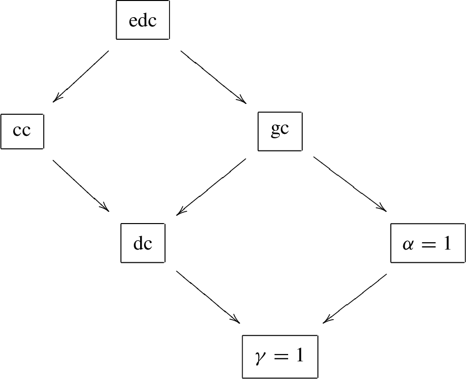
In Section 2 we discuss the relations among our four notions of asymptotic computation and their corresponding computability bounds, summarizing these in Fig. 1 and Theorem 2.5. In Section 3 we relativize our notions, and define corresponding reducibilities and degree structures. In Sections 4 and 5 we discuss natural embeddings of the Turing degrees into these degree structures and the resulting notion of quasiminimality, beginning by introducing some auxiliary notions related to the mod-finite and cofinite reducibilities of Dzhafarov and Igusa [6]. In Section 6 we study the sizes of upper cones and existence of minimal pairs in these structures. Hirschfeldt, Jockusch, Kuyper, and Schupp [8, Theorem 5.2] showed that nontrivial upper cones in the coarse degrees have measure 0, and used this fact to show the existence of minimal pairs in the coarse degrees. We show that nontrivial upper cones in the generic, dense, and effective dense degrees also have measure 0, and show the existence of minimal pairs in the dense degrees. Whether there are minimal pairs in the generic or effective dense degrees remains unknown. In Section 7, we gather several open questions.

In order to assist the reader in tracking the large number of notions defined in this paper, we collect summaries of the definitions in the Appendix.
2. Comparing notions of asymptotic computability

Our first order of business is to establish the relations between all four notions of asymptotic computability, including their corresponding computation bounds, which we summarize in Fig. 1.

Figure 1.

The graph of implications between notions of asymptotic computability, including computability bounds. All implications shown are strict, and all not shown are false. We have abbreviated coarse computability by “cc”, generic computability by “gc”, and (effective) dense computability by “(e)dc”.

We have already noted that effective dense computability implies both generic and coarse computability, which in turn both imply dense computability. Jockusch and Schupp [13, Proposition 2.15 and Theorem 2.26] showed that there are c.e. sets that are coarsely computable but not generically computable, and vice-versa, and hence that generic and coarse computability are incomparable. It follows that effective dense computability is strictly stronger than both generic and coarse computability, while dense computability is strictly weaker than both.

Turning to the bottom part of Fig. 1, we begin by showing that we do not need to add the computability bounds β and δ from Definition 1.6 to it.

Proposition 2.1.

Let $g : ω \to ω$ . Then $α (g) = β (g)$ and $γ (g) = δ (g)$ .

Proof.

Suppose g is partially computable at density d, as witnessed by the partial description f, and let $ε > 0$ . By Downey, Jockusch, and Schupp [5, Theorem 3.9], since $dom f$ is c.e., it has a computable subset B such that $\underline{ρ} (B) > \underline{ρ} (dom f) - ε$ . Let $h : ω \to ω \cup {□}$ be the total computable function defined by $\begin{matrix} h (n) = \{\begin{matrix} f (n) & if n \in B \\ □ & if n \notin B . \end{matrix} \end{matrix}$ Then h is a strong partial description of g with strong domain of lower density at least $d - ε$ . Since ε is arbitrary, we have $β (g) ⩾ α (g)$ . But clearly $α (g) ⩾ β (g)$ , so in fact $α (g) = β (g)$ .

Now suppose g is weakly partially computable at density d, as witnessed by the partial computable function f. Let $S = {n : f (n) = g (n)}$ and let $ε > 0$ . Again there is a computable $B \subseteq dom f$ such that $\underline{ρ} (B) > \underline{ρ} (dom f) - ε$ . Let h be the total computable function defined by $\begin{matrix} h (n) = \{\begin{matrix} f (n) & if n \in B \\ 0 & if n \notin B . \end{matrix} \end{matrix}$ Since $\underline{ρ} (S) ⩾ d$ and $S \subseteq dom f$ , we have $\underline{ρ} (S \cap B) ⩾ d - ε$ . Since $S \cap B \subseteq {n : h (n) = g (n)}$ , it follows that g is coarsely computable at density $d - ε$ . Since ε is arbitrary, we have $γ (g) ⩾ δ (g)$ . But clearly $δ (g) ⩾ γ (g)$ , so in fact $γ (g) = δ (g)$ . □

This result also provides the last remaining implication in Fig. 1.

Corollary 2.2.

If g is densely computable, then $γ (g) = 1$ .

To complete the justification of Fig. 1, it remains only to separate $α = 1$ from coarse and dense computability. As shown by Jockusch and Schupp [13, proof of Proposition 2.15], the usual construction of a simple set can be modified to yield a simple set A of density 0. Then A is coarsely computable but $α (A) = 0$ . Thus coarse computability does not imply $α = 1$ . We now separate $α = 1$ from dense computability.

Proposition 2.3.

There is a c.e. set A such that $α (A) = 1$ but A is not densely computable.

Proof.

Let A be defined as follows. For each $e, m \in ω$ such that $Φ_{e} (2^{e} k) = 0$ for at least half of the odd numbers $k < m$ , enumerate $2^{e} k$ into A for all odd numbers $k < m$ . Then, for each $e \in ω$ , either $2^{e} k \in A$ for all odd numbers k, or $2^{e} k \in A$ for only finitely many odd numbers k. From this fact it follows easily that $α (A) = 1$ .

Now fix $e \in ω$ . If there are infinitely many m such that $Φ_{e} (2^{e} k) = 0$ for at least half of the odd numbers $k < m$ , then for each such m, we have that $Φ_{e} (2^{e} k) = 0 \neq 1 = A (2^{e} k)$ for at least half of the odd numbers $k < m$ , and hence $Φ_{e}$ cannot be a dense description of A. Otherwise, for all sufficiently large m, for more than half of the odd numbers $k < m$ , we have that $Φ_{e} (2^{e} k)$ either diverges or converges to a number different from 0, while $A (2^{e} k) = 0$ . Again, $Φ_{e}$ cannot be a dense description of A. □

We thus have a full justification of the implications and nonimplications in Fig. 1, but we can actually say more. Jockusch and Schupp [13, Theorem 2.22] built a c.e. set of density 1 with no computable subset of density 1. Such a set is both generically and coarsely computable, but is not effectively densely computable. Thus effective dense computability is strictly stronger than the conjunction of generic and coarse computability. Paul Schupp [personal communication] showed that there is a c.e. set C such that C is densely computable but neither coarsely computable nor generically computable, which implies that dense computability is strictly weaker than the disjunction of generic and coarse computability. He obtained such a C as $A \oplus B$ , where A is coarsely computable but not generically computable and B is generically computable but not coarsely computable. This “join” method will be crucial in the proof of the more general Theorem 2.5 below. Subsequently but independently, Justin Miller [personal communication] showed that there is a set $C ⩽_{T} \emptyset^{'}$ such that C is densely computable but neither coarsely computable nor generically computable and, furthermore, $α (C) = 1$ .

In fact, we will show in Theorem 2.5 below that any Boolean combination of the properties in Fig. 1 is realizable by a c.e. set, provided it is not directly ruled out by the implications given in the figure. The following lemma, whose proof follows easily from the definitions, is basic to the proof.

Lemma 2.4.

Let P be any of the six properties in Fig. 1 . Then for any sets A and B, the property P holds of $A \oplus B$ if and only if P holds of both A and B.

Theorem 2.5.

Let V be the set of six vertices of the directed graph given in Fig. 1 . For $p, q \in V$ , define $q ⩽ p$ to mean that either $p = q$ or there is a directed path from p to q (so the property p implies the property q). Let P and Q be subsets of V. Then the following statements are equivalent:

There is a c.e. set that satisfies every $p \in P$ and no $q \in Q$ .

There is a set that satisfies every $p \in P$ and no $q \in Q$ .

There is a function that satisfies every $p \in P$ and no $q \in Q$ .

There do not exist $p \in P$ and $q \in Q$ such that $q ⩽ p$ .

Proof.

Clearly, (i) implies (ii), which in turn implies (iii), and it is immediate from the previous results of this section that (iii) implies (iv).

Now assume that (iv) holds in order to prove (i). Let M be the set of maximal elements of P under ⩽. Then P and M have the same downward closure under ⩽. It follows that the meaning of (iv) does not change if P is replaced by M. Also, the meaning of (i) does not change if P is replaced by M since, by the results of this section, the set of elements of V true of a given set C is closed downward and, again, P and M have the same downward closure. Thus, we assume without loss of generality that $P = M$ . Since M is an antichain and, by inspection of Fig. 1 all antichains have size at most 2, we have $| P | ⩽ 2$ . The result is easy if either P or Q is empty, so we may assume that $| P | \in {1, 2}$ .

Case 1. $| P | = 1$ . Let $P = {p}$ . For each $q \in Q$ , we do not have $q ⩽ p$ , so by the work of Jockusch and Schupp [13, Proposition 2.15 and its proof, and Theorem 2.26] discussed in the second paragraph of this section and in the paragraph before Proposition 2.3, together with Proposition 2.3 itself, there is a c.e. set $A_{q}$ that satisfies p but not q. Let $C = ⨁_{q \in Q} A_{q}$ . Then C witnesses (i), by Lemma 2.4.

Case 2. $| P | = 2$ . Since P is an antichain, it follows from inspection of Fig. 1 that P is one of the following three sets: ${c c, g c}$ , ${c c, α = 1}$ , and ${d c, α = 1}$ .

Case 2a. $P = {c c, g c}$ . Then, by (iv), $Q = {e d c}$ , so (i) asserts that there is a c.e. set C that is coarsely computable and generically computable but not effectively densely computable. The existence of such a set C follows from the discussion in the paragraph following Proposition 2.3, i.e., let C be a c.e. set of density 1 that has no computable subset of density 1.

Case 2b. $P = {c c, α = 1}$ . Then, by (iv), $Q \subseteq {e d c, g c}$ . Let B be a noncomputable c.e. set and let $C = {2^{n} k : n \in B \land k odd}$ . Then C is c.e., C is coarsely computable by Theorem 2.19 of [13], and $α (C) = 1$ as in the proof of Proposition 2.3. Also, since B is not computable, C is not generically computable by Observation 2.11 of [13]. Hence, C is also not effectively densely computable, and so witnesses that (i) holds.

Case 2c. $P = {d c, α = 1}$ . Then $Q \subseteq {c c, g c, e d c}$ by (iv). As shown in the previous case, there is a c.e. set A that is coarsely computable but not generically computable, and has $α (A) = 1$ . As mentioned above, Jockusch and Schupp [13, Theorem 2.26] showed that there is a c.e. set B that is generically computable but not coarsely computable. Note that both A and B are densely computable, and $α (B) = 1$ . Let $C = A \oplus B$ . By Lemma 2.4, C is densely computable but neither generically computable nor coarsely computable, and $α (C) = 1$ . It follows that C is also not effectively densely computable. So C witnesses that (i) holds.

Thus (i) holds in all cases and the proof is complete. □

3. Reducibilities related to asymptotic computation

Notions of asymptotic computability can be relativized. For instance, a function is coarsely computable relative to an oracle X if it has an X-computable coarse description. While this process does not yield transitive relations, we can also define transitive reducibilities based on our notions, capturing the idea of using partial information about a function to compute partial information about another. In each case, there are both a nonuniform and a uniform version, and there do not seem to be good reasons to prefer one over the other in general. For coarse and effective dense computability, the definitions are straightforward.

Definition 3.1.
We say that f is nonuniformly coarsely reducible to g, and write $f ⩽_{nc} g$ , if every coarse description of g computes a coarse description of f.

We say that f is uniformly coarsely reducible to g, and write $f ⩽_{uc} g$ , if there is a Turing functional Φ such that if d is a coarse description of g, then $Φ^{d}$ is a coarse description of f.

We say that f is nonuniformly effectively densely reducible to g, and write $f ⩽_{ned} g$ , if every effective dense description of g computes an effective dense description of f.

We say that f is uniformly effectively densely reducible to g, and write $f ⩽_{ued} g$ , if there is a Turing functional Φ such that if d is an effective dense description of g, then $Φ^{d}$ is an effective dense description of f.

Generic and dense descriptions are partial functions, so we cannot use them directly as oracles, but we can use their graphs. It would not make sense to use Turing functionals in defining generic and dense reducibility, however, because our reductions should not be able to use information about where partial functions are not defined. (For instance, from the graph of a dense description f of a set A, we can compute an effective dense description of A, since we can determine for any given n whether $f (n) ↓$ simply by checking whether $(n, 0) \in graph (f)$ or $(n, 1) \in graph (f)$ .) Thus we use enumeration operators, which can use only positive facts. Recall that an enumeration operator is a c.e. collection of pairs $(F, k)$ with each F finite. For an oracle X, let $W^{X} = {k : (\exists (F, k) \in W) F \subseteq X}$ . By definition, Y is enumeration reducible to X if there is an enumeration operator W such that $Y = W^{X}$ . For partial functions f and g, we say that f is enumeration reducible to g if $graph (f)$ is enumeration reducible to $graph (g)$ . Similarly, for partial functions f and g, if $W^{graph (g)} = graph (f)$ , we identify $W^{graph (g)}$ with f.
Definition 3.2.
We say that f is nonuniformly generically reducible to g, and write $f ⩽_{ng} g$ , if for every generic description d of g, there is a generic description e of f such that e is enumeration reducible to d.

We say that f is uniformly generically reducible to g, and write $f ⩽_{ug} g$ , if there is an enumeration operator W such that if d is a generic description of g, then $W^{graph (d)}$ is a generic description of f.

We say that f is nonuniformly densely reducible to g, and write $f ⩽_{nd} g$ , if for every dense description d of g, there is a dense description e of f such that e is enumeration reducible to d.

We say that f is uniformly densely reducible to g, and write $f ⩽_{ud} g$ , if there is an enumeration operator W such that if d is a dense description of g, then $W^{graph (d)}$ is a dense description of f.

Each of the reducibilities above induces an equivalence relation on $ω^{ω}$ (or on $2^{ω}$ , if we wish to consider sets rather than functions), from which a degree structure arises as usual. We will be concerned with the degrees of sets, but it is worth noting that, unlike in the case of the Turing degrees, it is not clear that the degrees of functions coincide with those of sets. (See Open Question 7.1.)

We also note that while nonimplications between notions of asymptotic computability immediately yield nonimplications between the corresponding reducibilities, the same is not true of implications. Thus several of the relationships between these reducibilities remain open. (See Open Question 7.2.) In the coarse and generic cases, Dzhafarov and Igusa have shown that uniform reducibility is strictly stronger than nonuniform reducibility (see [8, Theorems 2.6 and 2.7]). In Section 5 we will see that this fact is also true in the dense and effective dense cases.

A different and often more convenient approach to the definition of generic reducibility, which has been used in several papers, is to use Turing functionals but replace partial descriptions with time-dependent representations known as partial oracles. The same can be done for dense reducibility.
Definition 3.3.
Let $g : ω \to ω$ . A partial oracle for g is a set P such that if $⟨ n, k, s ⟩ \in P$ then $g (n) = k$ . A coarse partial oracle for g is a set that is a partial oracle for some coarse description of g. The domain of a partial oracle P is the set of n such that $⟨ n, k, s ⟩$ is in P for some k and s.

A generic oracle for g is a partial oracle for g with domain of density 1. A dense oracle for g is a coarse partial oracle for g with domain of density 1.

It is sometimes technically convenient to add to the definition of a partial oracle P the condition that for each n and k there is at most one s with $⟨ n, k, s ⟩ \in P$ , as is done in [3], but this modification does not change any of the notions defined using partial oracles.

It is easy to see that if $h ⩽_{ug} g$ then there is a Turing functional Φ such that if P is a generic oracle for g, then $Φ^{P}$ is a generic oracle for h, and that the analogous facts hold for $⩽_{ng}$ , $⩽_{ud}$ , and $⩽_{nd}$ . Conversely, Igusa [10, Proposition 3.10] (see also Cholak and Igusa [3, Observation 2.9]) showed that if such a Φ exists then $h ⩽_{ug} g$ . (He stated this fact for generic descriptions of sets rather than functions, but the argument works just as well in the more general setting of functions.) We now show that the analogous fact in the nonuniform case, which was left open in the above papers, also holds.
Proposition 3.4.
For all functions g and h, we have $h ⩽_{ng} g$ if and only if every generic oracle for g computes a generic oracle for h.
Proof.
As mentioned above, the “only if” direction is clear. Suppose that every generic oracle for g computes a generic oracle for h and fix a generic description f of g.

Say that $σ \in 2^{< ω}$ is acceptable if $σ (⟨ n, i, s ⟩) = 1 \Rightarrow f (n) = i$ . We force over the acceptable strings ordered by extension. Let G be sufficiently generic for this notion of forcing. If $σ ≺ G$ then σ is acceptable, so if $⟨ n, i, s ⟩ \in G$ then $f (n) = i$ , and hence $g (n) = i$ . Thus G is a partial oracle for g. If $f (n) = i$ then the set of acceptable σ such that $σ (⟨ n, i, s ⟩) = 1$ for some s is dense, and hence $⟨ n, i, s ⟩ \in G$ for some s. Thus $dom G \supseteq dom f$ , and hence $ρ (dom G) = 1$ .

Since G is a generic oracle for g, there is a Turing functional Φ such that $Φ^{G}$ is a generic oracle for h. Consider the set of acceptable σ such that there exist m, j, and t with $Φ^{σ} (⟨ m, j, t ⟩) = 1$ and $h (m) \neq j$ . No initial segment of G can be in this set, so G must avoid this set. That is, there is a $τ ≺ G$ such that for all acceptable $σ ≻ τ$ , if $Φ^{σ} (⟨ m, j, t ⟩) = 1$ then $h (m) = j$ .

Now define an enumeration operator W as follows. For each finite $F \subset ω \times ω$ , if there is a $σ ≻ τ$ (with σ not necessarily acceptable) such that $σ (⟨ n, i, s ⟩) = 1 \Rightarrow (n, i) \in F$ , and $Φ^{σ} (⟨ m, j, t ⟩) = 1$ , then add the pair $(F, (m, j))$ to W. If $X \subseteq ω \times ω$ is arbitrary, $W^{X}$ is just a relation, but when $X = graph (f)$ , we will show that this relation is single-valued, and hence is the graph of a partial function.

Let $d = W^{graph (f)}$ . If $F \subset graph (f)$ is finite, then any σ as in the previous paragraph is acceptable, so by the choice of τ, if $(m, j) \in d$ then $h (m) = j$ . In particular, d is single-valued, and we identify it with the partial function of which it is the graph. Thus to show that d is a generic description of h, it suffices to show that $ρ (dom d) = 1$ . If $m \in dom Φ^{G}$ then there is a σ with $τ ≺ σ ≺ G$ such that $Φ^{σ} (⟨ m, j, t ⟩) = 1$ for some j, t. Since σ is acceptable, there is a finite $F \subset graph (f)$ such that $(F, (m, j)) \in W$ , so $m \in dom d$ . Thus $dom d \supseteq dom Φ^{G}$ , and hence $ρ (dom d) = 1$ . □

Thus in both the uniform and nonuniform cases, the two ways to define generic reducibility agree. The above proof can easily be adapted to certain other reducibilities, such as the infinite-information reducibility introduced by Dzhafarov and Igusa [6]. Unfortunately, this is not the case for dense reducibility, as there seems to be no good analog to the existence of τ in that proof. Indeed, the aforementioned proofs in [10] and [3] for the uniform case also seem to fail for dense reducibility. Thus we do not know whether defining dense reducibility using dense oracles and Turing functionals would yield the same notions. (See Open Question 7.7.) Fortunately, the results in this paper do not depend on which version of dense reducibility we choose.
4. Cofinite reducibilities

As shown by Jockusch and Schupp [13], Dzhafarov and Igusa [6], and Hirschfeldt, Jockusch, Kuyper, and Schupp [8], there are natural embeddings of the Turing degrees into the coarse and generic degrees. As we will see in the next section, the same process works for the dense and effective dense degrees as well, by arguments similar to the ones in these papers. We will follow the version in [6], which filters through the notions of cofinite and mod-finite reducibility. In our case, we need to introduce two variants on those notions.

Definition 4.1.
A cofinite description of a function g is a partial description of g with cofinite domain. A function h is cofinitely reducible to a function g, written as $h ⩽_{cf} g$ , if there is an enumeration operator W such that if f is a cofinite description of g then $W^{graph (f)}$ is the graph of a cofinite description of h.

A mod-finite description of a function g is a function f such that $f (n) = g (n)$ for almost all n. A function h is mod-finitely reducible to a function g, written as $h ⩽_{mf} g$ , if there is a Turing functional Φ such that if f is a mod-finite description of g then $Φ^{f}$ is a mod-finite description of h.

A weak cofinite description of a function g is a cofinite description of a mod-finite description of g, i.e., a partial function f such that $f (n) = g (n)$ for almost all n. A function h is weak-cofinitely reducible to a function g, written as $h ⩽_{wcf} g$ , if there is an enumeration operator W such that if f is a weak cofinite description of g then $W^{graph (f)}$ is the graph of a weak cofinite description of h.

A strong cofinite description of a function g is a strong partial description of g with cofinite strong domain. A function h is strong-cofinitely reducible to a function f, written as $h ⩽_{scf} g$ , if there is a Turing functional Φ such that if f is a strong cofinite description of g then $Φ^{f}$ is a strong cofinite description of g.

In [6], the definitions of mod-finite and cofinite reducibility also required that $Φ^{g} = h$ , but as shown in that paper, dropping this condition does not affect either definition. Notice that the nonuniform version of each of these reducibilities is just Turing reducibility. These reducibilities induce degree structures in the usual way.

A cofinite oracle for a function g is a partial oracle for g with cofinite domain. The original definition of cofinite reducibility in [6] is in terms of cofinite oracles and Turing functionals, but essentially the same argument that shows that uniform generic reducibility is equivalent to the version defined using generic oracles shows that $h ⩽_{cf} g$ if and only if there is a Turing functional Φ such that if P is a cofinite oracle for g then $Φ^{P}$ is a cofinite oracle for h. We do not know whether the analogous fact holds for weak cofinite reducibility, however. (See Open Question 7.7.)

Our main interest in wcf-reducibility and scf-reducibility here is as tools in the study of dense and effective dense reducibility, but it is of independent interest to consider how they fit into the picture of measures of robust information coding in [6]. To begin to answer this question, we define another notion introduced in [6].
Definition 4.2.
We say that h is use-bounded-from-below reducible to g, and write $h ⩽_{ubfb} g$ , if h is computable from g via a functional Φ such that the smallest value of g queried in the computation of $Φ^{g} (n)$ goes to infinity with n.

Dzhafarov and Igusa [6, Theorem 3.1] showed that, in Cantor space, mf-reducibility strictly implies ubfb-reducibility, which in turn strictly implies cf-reducibility. Their proofs work in Baire space as well, except for the implication between mf-reducibility and ubfb-reducibility. Indeed, we have the following fact.
Proposition 4.3.
There are a function g and a set B such that $B ⩽_{mf} g$ but $B ≰_{cf} g$ , and hence $B ≰_{ubfb} g$ .
Proof.
We will define a function g and let $B = {⟨ n, k ⟩ : g (n) = k}$ . Then it is easy to see that $B ⩽_{mf} g$ .

We define g by finite extensions as follows. Suppose we have defined g on $[0, n]$ and want to ensure that $B ≰_{cf} g$ via a given enumeration operator W. Let $C$ be the class of all partial functions with finite domain that agree with g on $[0, n]$ and are undefined at $n + 1$ .

Case 1. There are a $k \in ω$ , an $i < 2$ , and an $f \in C$ such that $(⟨ n + 1, k ⟩, i) \in W^{graph (f)}$ . Let $g (n) = f (n)$ on the domain of f. Also, if $i = 0$ then let $g (n + 1) = k$ , and otherwise let $g (n + 1) = k + 1$ . This definition is consistent since $n + 1$ is not in the domain of f, and it ensures that $B (⟨ n + 1, k ⟩) \neq i$ . Finally, extend the definition of g so that the current domain of g is a finite initial segment of the natural numbers. Then $W^{graph (g)}$ contains $(⟨ n + 1, k ⟩, i)$ and so is not of the form $graph (h)$ for any partial description h of B.

Case 2. Otherwise. Then we simply set $g (n + 1) = 0$ . If $g_{0}$ is the partial function obtained from (the final version of) g by omitting $n + 1$ from its domain, then $g_{0}$ is a cofinite description of g such that $W^{graph (g_{0})}$ contains no number of the form $(⟨ n + 1, k ⟩, i)$ for $i < 2$ . Thus if $W^{graph (g_{0})}$ is the graph of a partial function h, then h cannot be defined as either 0 or 1 on $⟨ n + 1, k ⟩$ for any k, and hence h cannot be a cofinite description of any set. □

We also have the following implications.
Proposition 4.4.
If $h ⩽_{scf} g$ then $h ⩽_{ubfb} g$ .
Proof.
Suppose that $h ⩽_{scf} g$ via Φ. By finitely modifying Φ if necessary, we may assume that $Φ^{g} = h$ . Let $g_{n}$ be defined by letting $g_{n} (m) = □$ for $m < n$ and $g_{n} (m) = g (m)$ for $m ⩾ n$ . Note that $Φ^{g_{n}} (k) ↓ \in {h (k), □}$ for all n and k. We can compute h from g as follows. On input k, find the largest $n ⩽ k$ such that $Φ^{g_{n}} (k) \neq □$ (which must exist, since $Φ^{g_{0}} = Φ^{g} = h$ ). Then $h (k) = Φ^{g_{n}} (k)$ . This computation can be performed without querying $g (m)$ for any $m < n$ . For each n, we have that $Φ^{g_{n}}$ is a strong cofinite description of h, so $Φ^{g_{n}} (k) \neq □$ for almost all k. Thus the above procedure has use bounded from below. □
Proposition 4.5.
If $h ⩽_{ubfb} g$ then $h ⩽_{wcf} g$ .
Proof.
Suppose that $h ⩽_{ubfb} g$ via Φ. Define an enumeration operator W as follows. For each finite $F \subset ω \times ω$ and each n, run the computation of Φ on input n, and each time this computation queries its oracle on an input m, check whether $(m, j) \in F$ for some j. If not, or if this is the case for more than one j, then do nothing. Otherwise, provide the answer j to Φ’s query, and continue the computation. If this computation ever halts with an output i, then enumerate the pair $(F, (n, i))$ into W.

Let f be a weak cofinite description of g. Then f is a cofinite description of some mod-finite description d of g. If $(F, (n, i)) \in W$ for some $F \subset graph (f)$ then $Φ^{d} (n) = i$ , so $W^{graph (f)}$ is the graph of a partial function. Since Φ has its use bounded from below on oracle g, if n is sufficiently large then there is a finite $F \subset graph (f)$ such that all answers provided to Φ during the simulation described above are the same as Φ would get from g, and hence $(n, h (n)) \in W^{graph (f)}$ . Thus $W^{graph (f)}$ is a weak cofinite description of h. □
Corollary 4.6.
For functions g and h, if $h ⩽_{scf} g$ , then $h ⩽_{cf} g$ and $h ⩽_{wcf} g$ . For sets A and B, if $B ⩽_{mf} A$ , then $B ⩽_{cf} A$ and $B ⩽_{wcf} A$ .

Notice also that both wcf-reducibility and scf-reducibility are implied by 1-reducibility (for sets) and imply Turing reducibility. We do not know whether either of the implications in the above propositions is strict, or what the relationships between mf-reducibility and scf-reducibility, and between cf-reducibility and wcf-reducibility are. (See Open Question 7.8.)
5. Embeddings of the Turing degrees and quasiminimality

We can now define embeddings of the Turing degrees into each of our asymptotic reducibilities. Since every function is Turing equivalent to a set, we can work in Cantor space without loss of generality. Let $\begin{matrix} R (A) = {2^{n} k : n \in A \land k odd} . \end{matrix}$ Taking $J_{n} = [2^{n}, 2^{n + 1})$ , define $\begin{matrix} \tilde{R} (A) = ⋃_{n \in A} J_{n} . \end{matrix}$ Finally, let $E (A) = \tilde{R} (R (A))$ .

Dzhafarov and Igusa [6, Proposition 3.3] showed that $R$ induces embeddings of the Turing degrees into both the mod-finite and the cofinite degrees, and that $\tilde{R}$ induces embeddings of the cofinite degrees into the uniform generic degrees and of the mod-finite degrees into the uniform coarse degrees. A similar but easier argument shows that the latter map also induces embeddings of the Turing degrees into both the nonuniform generic and the nonuniform coarse degrees, since $\tilde{R} (A) \equiv_{T} A$ , and any coarse description of $\tilde{R} (A)$ or dense oracle for $\tilde{R} (A)$ computes A. Since $R (A) \equiv_{T} A$ , it follows that $E$ also induces these embeddings.

Thus we see that $E$ induces embeddings of the Turing degrees into the uniform and nonuniform generic and coarse degrees. (See [8, Proposition 2.2] for a proof that these embeddings are the unique ones with certain natural properties.) We now show that this is also the case for the uniform and nonuniform dense and effective dense degrees, by adapting the arguments in [6].

Lemma 5.1.

From the graph of a weak cofinite description of A we can uniformly enumerate the graph of a dense description of $\tilde{R} (A)$ , and vice-versa.

From a strong cofinite description of A we can uniformly compute an effective dense description of $\tilde{R} (A)$ , and vice-versa.

Proof.
Part 1: Suppose f is a weak cofinite description of A and define g by letting $g (m) = f (n)$ for $m \in J_{n}$ . The graph of g can be uniformly enumerated from the graph of f, and if $f (n) = A (n)$ then $g (m) = \tilde{R} (A) (m)$ for all $m \in J_{n}$ , so g is a weak cofinite description, and hence a dense description, of $\tilde{R} (A)$ .

Now suppose g is a dense description of $\tilde{R} (A)$ and define f as follows. For each n, if we see $g (m) = i$ for more than half of the elements of $J_{n}$ , then let $f (n) = i$ . The graph of f can be uniformly enumerated from the graph of g. If n is large enough, then $ρ_{2^{n + 1}} ({m : g (m) = \tilde{R} (A) (m)}) > \frac{3}{4}$ . Since $| J_{n} | = 2^{n}$ , it follows that $g (m) = A (n)$ for more than half of the elements of $J_{n}$ , and hence $f (n) = A (n)$ . Thus f is a weak cofinite description of A.

Part 2: Suppose f is a strong cofinite description of A and define g by letting $g (m) = f (n)$ for $m \in J_{n}$ . Then g can be uniformly computed from f, and if $f (n) = A (n)$ then $g (m) = \tilde{R} (A) (m)$ for all $m \in J_{n}$ , so g is a strong cofinite description, and hence an effective dense description, of $\tilde{R} (A)$ .

Now suppose g is an effective dense description of $\tilde{R} (A)$ and define the g-computable function f as follows. For each n, if $g (m) = i \neq □$ for some $m \in J_{n}$ then let $f (n) = i$ , and otherwise let $f (n) = □$ . (Notice that this definition makes sense, because if $m, m^{'} \in J_{n}$ and both $g (m) \neq □$ and $g (m^{'}) \neq □$ , then $g (m) = A (n) = g (m^{'})$ .) If $f (n) \neq □$ then $f (n) = \tilde{R} (A) (m)$ for some $m \in J_{n}$ , and hence $f (n) = A (n)$ . If n is large enough, then $ρ_{2^{n + 1}} ({m : g (m) = \tilde{R} (A) (m)}) > \frac{1}{2}$ . Since $| J_{n} | = 2^{n}$ , it follows that $g (m) = A (n)$ for some $m \in J_{n}$ , and hence $f (n) = A (n)$ . Thus f is a strong cofinite description of A. □
Proposition 5.2.

The map $\tilde{R}$ induces an embedding of the Turing degrees into the nonuniform dense degrees.

The map $\tilde{R}$ induces an embedding of the Turing degrees into the nonuniform effective dense degrees.

The map $\tilde{R}$ induces an embedding of the weak cofinite degrees into the uniform dense degrees.

The map $\tilde{R}$ induces an embedding of the strong cofinite degrees into the uniform effective dense degrees.

The map $R$ induces an embedding of the Turing degrees into the weak cofinite degrees, and hence $E$ induces an embedding of the Turing degrees into the uniform dense degrees.

The map $R$ induces an embedding of the Turing degrees into the strong cofinite degrees, and hence $E$ induces an embedding of the Turing degrees into the uniform effective dense degrees.

Proof.
Part 1: Suppose that $B ⩽_{T} A$ . From a dense description of $\tilde{R} (A)$ , we can (nonuniformly) recover A, and hence B, and hence $\tilde{R} (B)$ . Thus $\tilde{R} (B) ⩽_{nd} \tilde{R} (A)$ . Conversely, suppose that $\tilde{R} (B) ⩽_{nd} \tilde{R} (A)$ . From A we can compute $\tilde{R} (A)$ , and hence obtain a dense description of $\tilde{R} (B)$ , from which we can (nonuniformly) recover B. Thus $B ⩽_{T} A$ .

Part 2 follows by essentially the same argument.

Part 3: Suppose that $B ⩽_{wcf} A$ . By the first part of the lemma, given a dense description of $\tilde{R} (A)$ , we can uniformly recover a weak cofinite description of A, from which we can uniformly obtain a weak cofinite description of B, and hence, again by the first part of the lemma, uniformly obtain a dense description of $\tilde{R} (B)$ . The other direction is similar.

Part 4 follows by essentially the same argument, using the second part of the lemma.

Part 5: If $R (B) ⩽_{wcf} R (A)$ then $B \equiv_{T} R (B) ⩽_{T} R (A) \equiv_{T} A$ . Conversely, suppose that $Φ^{A} = B$ . Define the enumeration operator W as follows. For each finite $F \subset ω \times ω$ and each n and k, if there is a $σ \in 2^{< ω}$ such that $Φ^{σ} (n) ↓$ and for each $m < | σ |$ , we have $(2^{m} (2 (n + k) + 1), σ (m)) \in F$ , then enumerate the pair $(F, (2^{n} (2 k + 1), Φ^{σ} (n)))$ into W. Let f be a weak cofinite description of $R (A)$ . Then $W^{graph (f)}$ is the graph of a partial function g. If $n + k$ is sufficiently large, then $f (2^{m} (2 (n + k) + 1)) = A (m)$ for all m, and hence $g (2^{n} (2 k + 1)) = B (n)$ . Hence g is a weak cofinite description of $R (B)$ . Thus $R (B) ⩽_{wcf} R (A)$ .

Part 6 follows by a similar argument to part 5, using the fact that from a strong cofinite description of $R (A)$ , we can uniformly recover A. □

These embeddings can be used to separate the uniform and nonuniform versions of dense and effective dense reducibility. In the latter case, the proof is the same as the one for generic and coarse reducibility, due to Igusa (see [8, Theorems 2.6 and 2.7]) and based on results of Dzhafarov and Igusa [6]. Recall that a set X is autoreducible if there is a Turing functional Φ such that $Φ^{X ∖ {n}} (n) = X (n)$ for all n. Examples of sets that are not autoreducible include all 1-random sets (as shown by Figueira, Miller, and Nies [7, Proposition 8]) and all 1-generic sets (see [8, Proposition 2.5]).
Corollary 5.3.
There are sets A and B such that $A ⩽_{ned} B$ but $A ≰_{ued} B$ .
Proof.
Let X be a set that is not autoreducible, let $A = E (X)$ , and let $B = \tilde{R} (X)$ . By part 2 of Lemma 5.1, any effective dense description of B computes X, and hence computes A, so $A ⩽_{ned} B$ . Dzhafarov and Igusa [6, Proof of Proposition 4.6] showed that $R (X) ≰_{cf} X$ , so by Corollary 4.6, $R (X) ≰_{scf} X$ . Since $\tilde{R}$ induces an embedding of the scf-degrees into the ued-degrees, $A ≰_{ued} B$ . □

For dense reducibility, the analogous argument would filter through weak cofinite reducibility, and it is not clear that assuming that X is not autoreducible suffices to ensure that $R (X) ≰_{wcf} X$ . However, we can replace this assumption with a stronger one mentioned by Hirschfeldt, Jockusch, Kuyper, and Schupp [8, Section 2].
Definition 5.4.
A set X is jump-autoreducible if there is a Turing functional Φ such that $Φ^{{(X ∖ {n})}^{'}} (n) = X (n)$ for all n.

Not all sets are jump-autoreducible. Indeed, it was shown in an early version of [8] that 2-generic sets and 2-random sets are not jump-autoreducible. These proofs are not in the final version of that paper, as considering failures of jump-autoreducibility turned out not to be necessary in studying coarse and generic reducibility. Since we will use this concept in connection with dense reducibility, we include these proofs here.
Proposition 5.5 (Hirschfeldt, Jockusch, Kuyper, and Schupp).

If X is 2-generic, then X is not jump-autoreducible.

Proof.
Since X is 2-generic, X is 1-generic relative to $\emptyset^{'}$ . Hence, by the relativized version of the proof in [8, Proposition 2.5] that 1-generic sets are not autoreducible, X is not autoreducible relative to $\emptyset^{'}$ . However, the class of 1-generic sets is uniformly ${GL}_{1}$ , i.e., there exists a single Turing functional Ψ such that for every 1-generic X we have $Ψ^{X \oplus \emptyset^{'}} = X^{'}$ , as can be verified by looking at the usual proof that every 1-generic is ${GL}_{1}$ (see [12, Lemma 2.6]). Of course, if X is 1-generic, then $X ∖ {n}$ is also 1-generic for every n. Thus from an oracle for $(X ∖ {n}) \oplus \emptyset^{'}$ we can uniformly compute ${(X ∖ {n})}^{'}$ . Now, if X is jump-autoreducible, from ${(X ∖ {n})}^{'}$ we can uniformly compute $X (n)$ . Composing these reductions shows that $X (n)$ is uniformly computable from $(X ∖ {n}) \oplus \emptyset^{'}$ , which contradicts our previous remark that X is not autoreducible relative to $\emptyset^{'}$ . □

In the proof above we used the fact that the 2-generic sets are uniformly ${GL}_{1}$ . For 2-random sets this fact is almost true, as expressed by the following lemma. The proof is adapted from Monin [17, Proposition 4.2.5], where a generalization for higher levels of randomness is proved. Let $U_{0}, U_{1}, \dots$ be a fixed universal $\emptyset^{'}$ -Martin-Löf test, chosen so that from the index of any $\emptyset^{'}$ -Martin-Löf test $V_{0}, V_{1}, \dots$ and any n, we can compute an m such that $V_{m} \subseteq U_{n}$ . (The usual construction of a universal Martin-Löf test, as in [4, Theorem 6.2.5] for instance, yields such a test when relativized to $\emptyset^{'}$ .) The 2-randomness deficiency (with respect to $U_{0}, U_{1}, \dots$ ) of a 2-random X is the least c such that $X \notin U_{c}$ .
Lemma 5.6 (After Monin [17]).

There is a Turing functional Θ such that, for any 2-random X and any upper bound b on the 2-randomness deficiency of X, we have $Θ^{X \oplus \emptyset^{'}, b} = X^{'}$ .

Proof.
Let $V_{e} = {Z : e \in Z^{'}}$ . The $V_{e}$ are uniformly $Σ_{1}^{0}$ classes, so we can define a function $f ⩽_{T} \emptyset^{'}$ such that $μ (V_{e} ∖ V_{e} [f (e, i)]) < 2^{- i}$ for all e and i, where μ is Lebesgue measure on $2^{ω}$ . Then each sequence $V_{e} ∖ V_{e} [f (e, 0)]$ , $V_{e} ∖ V_{e} [f (e, 1)]$ , … is an $\emptyset^{'}$ -Martin Löf test, and from b we can compute a number m such that if X is 2-random and b bounds the 2-randomness deficiency of X, then $X \notin V_{e} ∖ V_{e} [f (e, m)]$ . Then $X \in V_{e}$ if and only if $X \in V_{e} [f (e, m)]$ , which we can verify $(X \oplus \emptyset^{'})$ -computably. □
Proposition 5.7 (Hirschfeldt, Jockusch, Kuyper, and Schupp).

If X is 2-random, then X is not jump-autoreducible.

Proof.
Let c be the 2-randomness deficiency of X. Because X is 2-random, it is not autoreducible relative to $\emptyset^{'}$ , as can be seen by relativizing the proof of Figueira, Miller, and Nies [7, Proposition 8] that no 1-random set is autoreducible. To obtain a contradiction, assume that X is jump-autoreducible via some functional Φ. Let $V_{e}^{n} = {X : X ∖ {n} \in U_{e + 1}}$ . It is easy to check that each $V_{0}^{n}, V_{1}^{n}, \dots$ is a $\emptyset^{'}$ -Martin-Löf test, and we can compute an index for this test from n. Thus there is a computable function f such that $V_{f (n) - 1}^{n} \subseteq U_{c}$ for all n. Then $X \notin V_{f (n) - 1}^{n}$ , so $X ∖ {n} \notin U_{f (n)}$ , and hence $f (n)$ bounds the 2-randomness deficiency of $X ∖ {n}$ . Now let $Ψ^{Y \oplus \emptyset^{'}} (n) = Φ^{Θ^{Y \oplus \emptyset^{'}, f (n)}} (n)$ , where Θ is as in Lemma 5.6. Then X is autoreducible relative to $\emptyset^{'}$ via Ψ, which is a contradiction. □
Corollary 5.8.
There are sets A and B such that $A ⩽_{nd} B$ but $A ≰_{ud} B$ .
Proof.
Let X be a set that is not jump-autoreducible, let $A = E (X)$ , and let $B = \tilde{R} (X)$ . Any dense description of B computes X, and hence computes A, so $A ⩽_{nd} B$ . It is now enough to show that $R (X) ≰_{wcf} X$ . Since $\tilde{R}$ induces an embedding of the wcf-degrees into the ud-degrees, it will then follow that $A ≰_{ud} B$ .

Assume for a contradiction that there is an enumeration operator W such that $W^{f}$ is a weak cofinite description of $R (X)$ for each weak cofinite description f of X. Given an oracle Y and an n, think of Y as a function and enumerate $W^{graph (Y)}$ . Let $g (n, s) = 0$ if at least half of the pairs $(2^{n} (2 k + 1), i)$ enumerated by stage s have $i = 0$ , and let $g (n, s) = 1$ otherwise. Let $g (n) = {lim}_{s} g (n, s)$ , or $g (n) ↑$ if this limit does not exist. We can uniformly compute the partial function g from $Y^{'}$ . If $Y = X ∖ {n}$ then Y is a weak cofinite description of X, so $W^{X}$ is a weak cofinite description of $R (X)$ , and hence $g (n) = X (n)$ . Thus we have a procedure for uniformly computing $X (n)$ from ${(X ∖ {n})}^{'}$ , contrary to hypothesis. □

Another issue that has attracted some attention recently is that of quasiminimality. For any of our asymptotic reducibilities r, an r-degree is quasiminimal if it is not zero and is not above any nonzero degree in the image of the embedding induced by $E$ . We expect the r-degrees of sufficiently random sets to be quasiminimal, because if X is not quasiminimal, then there is some noncomputable set that is computable from all partial versions of X (in whatever sense of partial version is appropriate to r), and it should not be possible to code a nontrivial amount of information into a random set in a sufficiently redundant way for such information recovery from partial versions to be possible. Indeed, Cholak and Igusa [3, Proposition 5.5] showed that every 1-random set has quasiminimal degree in both the uniform coarse and uniform generic degrees. Hirschfeldt, Jockusch, Kuyper, and Schupp [8, remarks after Corollary 3.3] showed that while this is not quite the case in general for the nonuniform coarse and generic degrees, every weakly 2-random set does have quasiminimal degree in the nonuniform coarse degrees. Cholak, Hirschfeldt, and Igusa (see [3, Theorem 6.3]) showed that this is also the case in the nonuniform generic degrees.

Hirschfeldt, Jockusch, Kuyper, and Schupp [8, Theorem 4.2] also showed that every 1-generic set has quasiminimal degree in both the uniform and nonuniform coarse degrees. Cholak and Igusa [3, Proposition 5.4] showed that this is also the case in the uniform generic degrees, and Cholak, Hirschfeldt, and Igusa (see [3, Proposition 6.9]) showed the same for the nonuniform generic degrees.

A special case of Corollary 3.14 in [8] is that if $X ⩽_{T} \emptyset^{'}$ is 1-random, then there is a promptly simple set A that is computable from every dense oracle for X. A similar proof to that of Proposition 3.4 then shows that for each dense description f of X, we have that $E (A)$ is enumeration reducible to f, which implies that $E (A) ⩽_{nd} X$ and $E (A) ⩽_{ned} X$ . Thus not every 1-random set has quasiminimal degree in the nonuniform dense or effective dense degrees. On the other hand, if $E (A) ⩽_{nd} X$ then A is computable from every dense oracle for X, and hence from every coarse description of X, which implies that $E (A) ⩽_{nc} X$ . Thus the fact that every weakly 2-random or 1-generic set has quasiminimal degree in the nonuniform coarse degrees implies that the same is true in the nonuniform dense degrees, and hence in the uniform dense degrees. Whether 1-randomness suffices to ensure quasiminimality in the uniform dense degrees remains open. (See Open Question 7.4.)

Cholak and Igusa [3, Propositions 5.4 and 5.5] showed that if a set is 1-random or 1-generic, then it is quasiminimal in the cofinite degrees (with respect to the embedding $R$ ). Since scf-reducibility implies cf-reducibility, such a set must also be quasiminimal in the strong-cofinite degrees, and hence in the uniform effective dense degrees.

As mentioned above, Cholak, Hirschfeldt, and Igusa (see [3]) showed that 1-generic sets are quasiminimal for nonuniform generic reducibility, as are weakly 2-random sets. By forcing an effective dense oracle in place of their generic oracle, their methods also apply to nonuniform effective dense reducibility. Thus we have the following theorem.
Theorem 5.9 (Including results of Hirschfeldt, Jockusch, Kuyper, and Schupp [8]; Cholak and Igusa [3]; and Cholak, Hirschfeldt, and Igusa (see [3])).

Every weakly 2-random or 1-generic set is quasiminimal in all of the asymptotic degree structures considered here. Every 1-random set is quasiminimal in the uniform generic, coarse, and effective dense degrees, but there are 1-random sets that are not quasiminimal in the nonuniform generic, coarse, dense, and effective dense degrees.

This theorem leaves open only the aforementioned question of whether there are 1-random sets that are not quasiminimal in the uniform dense degrees.

It should also be noted that, as shown by Igusa (see [8, Theorem 4.3]), if $γ (X) = 1$ (so in particular if X is densely computable) but X is not coarsely computable, then X has quasiminimal degree in both the uniform and nonuniform coarse degrees.

6. Measure, upper cones, and minimal pairs

We now consider the sizes of upper cones and existence of minimal pairs in settings arising from notions of asymptotic computability. A reason for studying these issues in conjunction is given by the work of Hirschfeldt, Jockusch, Kuyper, and Schupp [8]. They showed in [8, Theorem 5.2] that if $A \in 2^{ω}$ is not coarsely computable, then the class of $X \in 2^{ω}$ such that A is coarsely computable relative to X has measure 0, and indeed does not contain any set that is weakly 3-random relative to A. They then used this result to show that if X is not coarsely computable and Y is weakly 3-random relative to X, then any set that is coarsely computable relative both to X and to Y must be coarsely computable. In this case, we say that X and Y form a minimal pair for relative coarse computability (and similarly for our other notions of asymptotic computation). It follows that X and Y also form a minimal pair in the (uniform or nonuniform) coarse degrees of sets.

Earlier, Downey, Jockusch, and Schupp [5, Section 7] asked whether there are minimal pairs in the uniform generic degrees. This question is still open, in both the uniform and nonuniform cases (see Open Question 7.3), but a partial answer was given by Igusa [10, Theorem 2.1], who showed that there are no minimal pairs for relative generic computability.

In this section, we extend the upper cone result in [8, Theorem 5.2] to all of our notions of asymptotic computation. For dense computability (but not for generic or effective dense computability), we will then be able to adapt the method in [8] to prove the existence of minimal pairs, though at a higher level of randomness.

We begin with a technical result that provides a modified version of Fubini’s Theorem constraining the relation between asymptotic density and Lebesgue measure on Cantor space. For a sequence $S = {S_{n}}_{n \in ω}$ of Lebesgue-measurable subsets of $2^{ω}$ and a set $A \subseteq ω$ , let $S (A) = {n : A \in S_{n}}$ . Let μ denote Lebesgue measure on Cantor space.

Lemma 6.1.
Let a, b, q, and $S = {S_{n} \subseteq 2^{ω}}_{n \in ω}$ be such that $\begin{matrix} \overline{ρ} ({n : μ (S_{n}) < q}) > a \end{matrix}$ and $\begin{matrix} μ ({A : ρ (S (A)) = 1}) > b . \end{matrix}$ Then $(1 - q) a + b ⩽ 1$ .
Proof.
Fix $r < 1$ and let $\begin{matrix} X_{n} = {A : (\forall k > n) ρ_{k} (S (A)) > r} . \end{matrix}$ Since the union of these classes contains ${A : ρ (S (A)) = 1}$ , it must have measure greater than b; since the classes are nested, there must be some N such that $μ (X_{n}) > b$ for all $n > N$ .

As the set of j such that $μ (S_{j}) < q$ has upper density greater than a, there must be some $n > N$ such that $μ (S_{j}) < q$ for at least $n a$ many $j < n$ .

As integration commutes with finite sums, $\begin{matrix} (1) & \frac{1}{n} \sum_{j < n} \int_{2^{ω}} 1_{S_{j}} d μ = \int_{2^{ω}} \frac{1}{n} \sum_{j < n} 1_{S_{j}} d μ, \end{matrix}$ where $1_{S_{j}} : 2^{ω} \to {0, 1}$ is 1 on $S_{j}$ and 0 elsewhere. Furthermore, $\begin{matrix} \frac{1}{n} \sum_{j < n} \int_{2^{ω}} 1_{S_{j}} d μ = \frac{1}{n} \sum_{j < n} μ (S_{j}) . \end{matrix}$ By our choice of n, there are at least $n a$ many $j < n$ for which $μ (S_{j}) < q$ ; for the remaining $S_{j}$ , we can still bound their measure by $μ (S_{j}) ⩽ 1$ . Therefore, $\begin{matrix} \frac{1}{n} \sum_{j < n} μ (S_{j}) < \frac{1}{n} (1 (n - n a) + q (n a)) = (1 - a) + q a = 1 - (1 - q) a . \end{matrix}$ On the other hand, considering the right-hand side of equation (1), we have $\begin{matrix} \int_{2^{ω}} \frac{1}{n} \sum_{j < n} 1_{S_{j}} d μ = \int_{A \in 2^{ω}} ρ_{n} (S (A)) d μ ⩾ \int_{A \in X_{n}} ρ_{n} (S (A)) d μ > μ (X_{n}) r > b r . \end{matrix}$

Therefore, $1 - (1 - q) a > b r$ and hence $(1 - q) a + b r < 1$ . Since $r < 1$ is arbitrary, $(1 - q) a + b ⩽ 1$ . □

The following statement puts the above result into a more useful form for our purposes.
Proposition 6.2.
Let $S = {S_{n} \subseteq 2^{ω}}_{n \in ω}$ and q be such that $\begin{matrix} μ ({A \in 2^{ω} : ρ (S (A)) = 1}) > q . \end{matrix}$ Then $\begin{matrix} ρ ({n : μ (S_{n}) ⩾ q}) = 1 . \end{matrix}$
Proof.
If $q = 0$ then the statement is trivial, so we may assume that $q > 0$ . Let $p = \overline{ρ} ({n : μ (S_{n}) < q})$ and assume for a contradiction that $p > 0$ . Let $ε > 0$ be such that $\frac{1}{p ε} \in N$ and $\begin{matrix} μ ({A \in 2^{ω} : ρ (S (A)) = 1}) > q + ε . \end{matrix}$

Let $I = {n_{0} < n_{1} < \dots}$ be the sequence of all n such that either $μ (S_{n}) < q$ or $n \equiv 0 (mod \frac{1}{p ε})$ . Then I has lower density at least $p ε$ and upper density at most $p (1 + ε)$ . We now pass to the subsequence $T = {S_{n_{j}}}_{j \in ω}$ . Since I has positive lower density, every set of density 1 must intersect I with density 1 within I, so $\begin{matrix} μ ({A \in 2^{ω} : ρ (T (A)) = 1}) > q + ε . \end{matrix}$ Since the upper density of I is at most $p (1 + ε)$ , given any $δ > 0$ , there is some N so that for all $n > N$ , we have $ρ_{n} (I) < p (1 + ε) + δ$ . However, I contains all n such that $μ (S_{n}) < q$ ; these form a set G of upper density p by assumption, and we have $ρ_{n} (G) > p - δ$ for infinitely many n.

Fix any $n > N$ such $ρ_{n} (G) > p - δ$ and let k be least such that $n_{k} ⩾ n$ . Then $\begin{matrix} ρ_{k} ({j : μ (S_{n_{j}}) < q}) = ρ_{k} ({j : n_{j} \in G}) = \frac{ρ_{n} (G \cap I)}{ρ_{n} (I)} = \frac{ρ_{n} (G)}{ρ_{n} (I)} > \frac{p - δ}{p (1 + ε) + δ} . \end{matrix}$ We therefore see that $\begin{matrix} \overline{ρ} ({j : μ (S_{n_{j}}) < q}) ⩾ \frac{p - δ}{p (1 + ε) + δ} = \frac{1 - \frac{δ}{p}}{1 + ε + \frac{δ}{p}} . \end{matrix}$ Since this inequality holds for all $δ > 0$ , we must have $\begin{matrix} \overline{ρ} ({j : μ (S_{n_{j}}) < q}) ⩾ \frac{1}{1 + ε} > 1 - ε . \end{matrix}$

Let $a = 1 - ε$ and $b = q + ε$ . Then $(1 - q) a + b = (1 - q) (1 - ε) + q + ε = 1 + q ε > 1$ , and $T$ has the properties in the statement of Lemma 6.1, yielding the desired contradiction. □

This result is the foundation for our arguments in the remainder of this section, as it allows us to use majority-vote arguments to construct computable asymptotic descriptions of sets with positive-measure upper cones. We first apply this technique to generic computability.
Theorem 6.3.
If $f : ω \to ω$ is not generically computable then $\begin{matrix} μ ({X : f is generically computable relative to X}) = 0 . \end{matrix}$ Indeed, no element of this set can be weakly 4-random relative to f. Thus all nontrivial upper cones in the (uniform or nonuniform) generic degrees of sets have measure 0.
Proof.
For a functional Φ, let $\begin{matrix} F_{Φ} = {X : Φ^{X} is a generic description of f} . \end{matrix}$ Then $F_{Φ}$ is a $Π_{4}^{0, f}$ -class, as $X \in F_{Φ}$ if and only if
for every n and s, if $Φ^{X} (n) [s] ↓$ then $Φ^{X} (n) = f (n)$ and

for every k there is an N such that for every $n > N$ there is an s for which $ρ_{n} (dom Φ^{X} [s]) > 1 - \frac{1}{k}$ .
Thus it suffices to fix Φ and show that $μ (F_{Φ}) = 0$ .

Assume for a contradiction that $μ (F_{Φ}) > 0$ . By Lebesgue Density (see e.g. [4, Theorem 1.2.3]), we may assume that $μ (F_{Φ}) > \frac{2}{3}$ . Let $S_{n} = {X : Φ^{X} (n) = f (n)}$ and let $S = {S_{n}}_{n \in ω}$ . Since $μ ({X : ρ (S (X)) = 1}) ⩾ μ (F_{Φ}) > \frac{2}{3}$ , Proposition 6.2 implies that $μ (S_{n}) ⩾ \frac{2}{3} > \frac{1}{2}$ for density-1 many n. We use this fact to compute a generic description of f, using a majority-vote scheme.

For each n, we wait until we see that there is an i and a class $C$ of measure greater than $\frac{1}{2}$ such that for some i and each $X \in C$ , we have $Φ^{X} (n) = i$ , and define $d (n) = i$ . (There may not be such an i, but note that for each n there is at most one such i.) Then d is a partial computable function, and $d (n)$ can never converge to a value other than $f (n)$ , as otherwise we would have a class of measure greater than $\frac{1}{2}$ disjoint from $F_{Φ}$ . Furthermore, for each of the density-1 many n such that $μ (S_{n}) > \frac{1}{2}$ , we have that $d (n) ↓$ . Thus d is a partial computable generic description of f. □

A similar proof gives us the same result for dense computability.
Theorem 6.4.
If $f : ω \to ω$ is not densely computable then $\begin{matrix} μ ({X : f is densely computable relative to X}) = 0 . \end{matrix}$ Indeed, no element of this set can be weakly 4-random relative to f. Thus all nontrivial upper cones in the (uniform or nonuniform) dense degrees of sets have measure 0.
Proof.
For a ${0, 1}$ -valued functional Φ, let $\begin{matrix} F_{Φ} = {X : Φ^{X} is a dense description of f} . \end{matrix}$ We again have that $F_{Φ}$ is a $Π_{4}^{0, f}$ -class, as $X \in F_{Φ}$ if and only if for every k there is an N such that for every $n > N$ there is an s for which $ρ_{n} ({m : Φ^{X} [s] (m) = f (m)}) > 1 - \frac{1}{k}$ .

Assume for a contradiction that $μ (F_{Φ}) > 0$ . We again may assume that $μ (F_{Φ}) > \frac{2}{3}$ , define $S_{n}$ as before, and conclude that $μ (S_{n}) > \frac{1}{2}$ for density-1 many n. We then define the partial computable function d as before. If $d (n) ↑$ or $d (n) ↓ \neq f (n)$ , then the class of all X such that $Φ^{X} (n) ↑$ or $Φ^{X} (n) ↓ \neq f (n)$ has measure greater than $\frac{1}{2}$ , which implies that $μ (S_{n}) < \frac{1}{2}$ , so there can be only density-0 many such n. Thus d is a partial computable dense description of f. □

In the case of effective dense computability, we can again use a similar argument, but the level of randomness needed is lower (as in the case of coarse computability).
Theorem 6.5.
If $f : ω \to ω$ is not effectively densely computable then $\begin{matrix} μ ({X : f is effectively densely computable relative to X}) = 0 . \end{matrix}$ Indeed, no element of this set can be weakly 3-random relative to f. Thus all nontrivial upper cones in the (uniform or nonuniform) effective dense degrees of sets have measure 0.
Proof.
For an $(ω \cup {□})$ -valued functional Φ, let $\begin{matrix} F_{Φ} = {X : Φ^{X} is an effective dense description of f} . \end{matrix}$ In this case, $F_{Φ}$ is a $Π_{3}^{0, f}$ -class, as $X \in F_{Φ}$ if and only if
for every n there is an s such that $Φ^{X} (n) [s] ↓ \in {f (n), □}$ and

for every k there is an N such that for every $n > N$ and every s, if $Φ^{X} (m) [s] ↓$ for all $m < n$ , then $ρ_{n} ({m : Φ^{X} [s] (m) = □}) < \frac{1}{k}$ .

Assume for a contradiction that $μ (F_{Φ}) > 0$ . We may then assume that $μ (F_{Φ}) > \frac{2}{3}$ , define $S_{n}$ as before, and conclude that $μ (S_{n}) ⩾ \frac{2}{3}$ for density-1 many n. For each n, we wait until we see a class of measure greater than $\frac{1}{3}$ such that for some $i \in ω \cup {□}$ and each X in this class, we have $Φ^{X} (n) = i$ , and define $d (n) = i$ . (There may be more than one i for which such a class exists, but we choose the first one we find.) If $X \in F_{Φ}$ , then $Φ^{X}$ is total and $Φ^{X} (n) \in {f (n), □}$ for all n, so for each n, there are either more than measure- $\frac{1}{3}$ many X such that $Φ^{X} (n) = f (n)$ or more than measure- $\frac{1}{3}$ many X such that $Φ^{X} (n) = □$ . Thus d is a total computable function and $d (n) \in {f (n), □}$ for all n. For each of the density-1 many n such that $μ (S_{n}) ⩾ \frac{2}{3}$ , there are at most measure- $\frac{1}{3}$ many X such that $Φ^{X} (n) = □$ , so $d (n) \neq □$ . Thus d is a computable effective dense description of f. □

We can also use a similar argument to give a different proof of the analogous result for coarse computability proved in [8, Theorem 5.2]. This argument is simpler than the original proof, given Proposition 6.2, and also applies to functions.
Theorem 6.6 (Hirschfeldt, Jockusch, Kuyper, and Schupp [8]).

If $f : ω \to ω$ is not coarsely computable then $\begin{matrix} μ ({X : f is coarsely computable relative to X}) = 0 . \end{matrix}$ Indeed, no element of this set can be weakly 3-random relative to f. Thus all nontrivial upper cones in the (uniform or nonuniform) coarse degrees of sets have measure 0.

Proof.
For a functional Φ, let $\begin{matrix} F_{Φ} = {X : Φ^{X} is a coarse description of f} . \end{matrix}$ As noted in [8, proof of Theorem 5.2], $F_{Φ}$ is a $Π_{3}^{0, f}$ -class. (The argument there was given for the case of a ${0, 1}$ -valued f, but clearly applies in general.) Assume for a contradiction that $μ (F_{Φ}) > 0$ . We may assume that $μ (F_{Φ}) > \frac{3}{4}$ , define $S_{n}$ as before, and conclude that $μ (S_{n}) ⩾ \frac{3}{4}$ for density-1 many n. Define d as follows. For each n, wait until we see a class $C$ of measure at least $\frac{3}{4}$ such that $Φ^{X} (n) ↓$ for all $X \in C$ . If there is an i such that $Φ^{X} (n) = i$ for at least measure- $\frac{1}{2}$ many $X \in C$ , then let $d (n) = i$ . Otherwise, let $d (n) = 0$ . Note that, if $d (n) ↓ \neq f (n)$ , then $μ (C \cap S_{n}) < \frac{1}{2}$ , so $μ (S_{n}) < \frac{3}{4}$ .

Since $Φ^{X}$ is total for more than measure- $\frac{3}{4}$ many X, the function d is a total computable function. If $d (n) \neq f (n)$ then, as noted above, $μ (S_{n}) < \frac{3}{4}$ , so there can be only density-0 many such n. Thus d is a computable coarse description of f. □

It was shown in [8, Theorem 5.6] that the weak 3-randomness condition in this theorem cannot in general be brought down to 2-randomness, but we do not know whether the levels of randomness needed for the other theorems in this section can be decreased. (See Open Question 7.5.)

As mentioned above, Theorem 6.6 has as a consequence that if X is not coarsely computable and Y is weakly 3-random relative to X, then X and Y form a minimal pair for relative coarse computability, and hence for both uniform and nonuniform coarse reducibility. A variant on the proof of Corollary 5.3 in [8] allows us to establish an analogous result for dense computability. The coarse computability proof is based on the observation that any two coarse descriptions of the same set are necessarily coarse descriptions of each other. The analogous statement makes little sense for dense descriptions, as these are partial functions. However, by careful choice of a completion of a dense description, we can recover the construction of minimal pairs as a consequence of Theorem 6.4 without increasing the level of randomness involved.
Corollary 6.7.
If Y is not densely computable and X is weakly 4-random relative to Y, then X and Y form a minimal pair for relative dense computability (and hence for both uniform and nonuniform dense reducibility).
Proof.
If f is a partial computable function with $ρ (dom f) = 1$ , then, as noted in the proof of Proposition 2.1, $dom f$ has a computable subset S of positive lower density. Since X is 1-random, the density within S of numbers n such that $f (n) \neq X (n)$ must be $\frac{1}{2}$ , and hence the overall density of such n is positive. Thus X is not densely computable.

Now suppose that C is densely computable relative both to X and to Y. Fix dense descriptions $Φ^{X}$ and $Ψ^{Y}$ of C. Let P be a set that is both PA over Y and low relative to Y. Then P computes a ${0, 1}$ -valued completion D of $Ψ^{Y}$ . Since D agrees with C on a set of density 1, we have that $Φ^{X}$ is a dense description of D, and hence D is densely computable relative to X. However, D is P-computable, and hence is low relative to Y, so X is weakly 4-random relative to D. By Theorem 6.4, D must be densely computable. Since any dense description of D is also a dense description of C, it follows that C is densely computable. □

By the aforementioned result of Igusa [10], this method of constructing minimal pairs cannot work for generic computability. It also does not seem to work for effective dense computability, at least not in any straightforward way. (See Open Question 7.3.) It is worth noting, however, that if Y is not generically computable, X is weakly 4-random relative to Y, and C is generically computable relative to both X and Y then, by Corollary 6.7, C is densely computable. In other words, there are pairs of sets X, Y such that all witnesses to the fact that X and Y do not form a minimal pair for relative generic computability are in a sense “close to generically computable”.

We can also consider the sizes of upper cones in the sense of category. Here we know less than in the case of measure, but do have the following results.
Theorem 6.8.
If f is not generically computable and X is 1-generic relative to f then X does not compute a generic description of f. Thus all nontrivial upper cones in the (uniform or nonuniform) generic degrees are meager.
Proof.
Suppose that X is 1-generic relative to f and $Φ^{X}$ is a generic description of f. The set of $σ \in 2^{< ω}$ such that $Φ^{σ} (n) ↓ \neq f (n)$ for some n is f-c.e. Since X does not meet this set, it must avoid it. Thus there is a $τ ≺ X$ such that for all $σ ≻ τ$ , if $Φ^{σ} (n) ↓$ then $Φ^{σ} (n) = f (n)$ . Define a partial computable function d by searching for strings $σ ≻ τ$ and numbers n such that $Φ^{σ} (n) ↓$ and letting $d (n) = Φ^{σ} (n)$ . Then d is a partial description of f. Since $τ ≺ X$ , we have $dom Φ^{X} \subseteq dom d$ , so $ρ (dom d) = 1$ . Thus d is a partial computable generic description of f. □

For the next result, we will use the following lemma from [9]. Let $J_{k}$ be the interval $[2^{k} - 1, 2^{k + 1} - 1)$ . For a set C, let $d_{k} (C)$ be the density of C on $J_{k}$ , that is, $\frac{| C \cap J_{k} |}{2^{k}}$ . Let $\overline{d} (C) = {lim sup}_{k} d_{k} (C)$ .
Lemma 6.9 (Hirschfeldt, Jockusch, McNicholl, and Schupp [9, Lemma 5.9]).

For every set C, we have $\frac{\overline{d} (C)}{2} ⩽ \overline{ρ} (C) ⩽ 2 \overline{d} (C)$ .

Let $γ^{X}$ be the relativization of the coarse computability bound γ to the set X.

Theorem 6.10.
If $γ (f) < 1$ and X is 1-generic relative to f then $γ^{X} (f) < 1$ .
Proof.
Suppose X is 1-generic relative to f and $γ^{X} (f) = 1$ . Let $ε > 0$ be rational. Let Φ be a functional such that $Φ^{X}$ is total and $\overline{ρ} ({n : Φ^{X} (n) \neq f (n)}) < ε$ . Then there is an M such that if $m > M$ then $ρ_{m} ({n : Φ^{X} (n) \neq f (n)}) < ε$ . Let S be the set of all $σ \in 2^{< ω}$ for which there is an $m > M$ such that $Φ^{σ} (n) ↓$ for all $n < m$ and $ρ_{m} ({n : Φ^{σ} (n) ↓ \neq f (n)}) ⩾ ε$ . Then S is f-c.e., and X does not meet S, so X must avoid S. That is, there is a $τ ≺ X$ such that for all $σ ≻ τ$ , we have $σ \notin S$ .

Now define a computable function g as follows. Let $J_{k}$ be as above. For each k in turn, search for a $σ ≻ τ$ such that $Φ^{σ} (n) ↓$ for all $n < 2^{k + 1}$ . Such a σ must exist because $τ ≺ X$ and $Φ^{X}$ is total. Once σ is found, let $g (n) = Φ^{σ} (n)$ for all $n \in J_{k}$ . If $2^{k + 1} ⩾ M$ then, by the choice of τ, we have $ρ_{2^{k + 1} + 1} ({n : Φ^{σ} (n) \neq f (n)}) < ε$ . Since $| J_{k} | = 2^{k}$ , it follows that $d_{k} ({n : g (n) \neq f (n)}) = d_{k} ({n : Φ^{σ} (n) \neq f (n)}) < 2 ε$ . Thus $\overline{d} ({n : g (n) \neq f (n)}) ⩽ 2 ε$ , so by Lemma 6.9, $\overline{ρ} ({n : g (n) \neq f (n)}) ⩽ 4 ε$ , and hence $γ (f) ⩾ 1 - 4 ε$ . Since ε is arbitrary, $γ (f) = 1$ . □

7. Open questions

In this final section, we gather some questions left open in this paper. We order these in decreasing order of how basic we believe they are to the emerging theory of dense computability.

Open Question 7.1.

For each reducibility r among the ones defined in Section 3, is it the case that every function is r-equivalent to a set?

Open Question 7.2.

The following questions can be asked in both uniform and nonuniform versions: Does effective dense reducibility imply generic reducibility? Does effective dense reducibility imply coarse reducibility? Does generic reducibility imply dense reducibility? Does coarse reducibility imply dense reducibility? Does effective dense reducibility imply dense reducibility?

More generally, how do effective dense reducibility and dense reducibility fit into the picture of implications between notions of robust information coding given by Dzhafarov and Igusa [6]?

Open Question 7.3.

Are there minimal pairs in the (uniform or nonuniform) generic or effective dense degrees? Are there minimal pairs for relative effective dense computability?

Open Question 7.4.

Do all 1-random sets have quasiminimal degree in the uniform dense degrees?

Open Question 7.5.

Can the weak 4-randomness condition in Theorems 6.3 and 6.4, and Corollary 6.7, or the weak 3-randomness condition in Theorem 6.5 be improved?

Open Question 7.6.

Are there analogs of Theorem 6.8 for coarse, dense, and effective dense computability? In particular, are nontrivial upper cones in the coarse, dense, and effective dense degrees meager?

Open Question 7.7.

If $h ⩽_{nd} g$ , does every dense oracle for g compute a dense oracle for h? If $h ⩽_{ud} g$ , does every dense oracle for g uniformly compute a dense oracle for h?

A weak cofinite oracle for a function g is a cofinite oracle for a mod-finite description of g. If $h ⩽_{wcf} g$ , does every weak cofinite oracle for g uniformly compute a weak cofinite oracle for h?

Open Question 7.8.

The following questions can be asked in Cantor space or in Baire space: Do either of mf-reducibility and scf-reducibility imply the other? Do either of cf-reducibility and wcf-reducibility imply the other? Does ubfb-reducibility imply scf-reducibility? Does wcf-reducibility imply ubfb-reducibility?

Does mf-reducibility imply wcf-reducibility in Baire space?

Footnotes

Acknowledgements

Hirschfeldt was partially supported by grants DMS-1101458 and DMS-1600543 from the National Science Foundation of the United States, and a Collaboration Grant for Mathematicians from the Simons Foundation.

Defined notions

References

Andrews,

Cai,

Diamondstone,

Jockusch and

Lempp, Asymptotic density, computable traceability, and 1-randomness, Fund. Math. 234 (2016), 41–53.

Astor, Asymptotic density, immunity, and randomness, Computability 4 (2015), 141–158. doi:10.3233/COM-150040.

Cholak and

Igusa, Density-1-bounding and quasiminimality in the generic degrees, J. Symbolic Logic 82 (2017), 931–957. doi:10.1017/jsl.2016.50.

R.G.

Downey and

D.R.

Hirschfeldt, Algorithmic Randomness and Complexity, Theory and Applications of Computability, Springer, New York, 2010.

R.G.

Downey,

C.G.

JockuschJr. and

P.E.

Schupp, Asymptotic density and computably enumerable sets, J. Math. Log 13 (2013), 1350005, 43 pp. doi:10.1142/S0219061313500050.

D.D.

Dzhafarov and

Igusa, Notions of robust information coding, Computability 6 (2017), 105–124. doi:10.3233/COM-160059.

Figueira,

J.S.

Miller and

Nies, Indifferent sets, J. Logic Comput. 19 (2009), 425–443. doi:10.1093/logcom/exn101.

D.R.

Hirschfeldt,

C.G.

JockuschJr.,

Kuyper and

P.E.

Schupp, Coarse reducibility and algorithmic randomness, J. Symbolic Logic 81 (2016), 1028–1046. doi:10.1017/jsl.2015.70.

D.R.

Hirschfeldt,

C.G.

JockuschJr.,

McNicholl and

P.E.

Schupp, Asymptotic density and the coarse computability bound, Computability 5 (2016), 13–27. doi:10.3233/COM-150035.

10.

Igusa, Nonexistence of minimal pairs for generic computation, J. Symbolic Logic 78 (2013), 511–522. doi:10.2178/jsl.7802090.

11.

Igusa, The generic degrees of density-1 sets, and a characterization of the hyperarithmetic reals, J. Symbolic Logic 80 (2015), 1290–1314. doi:10.1017/jsl.2014.77.

12.

C.G.

JockuschJr., Degrees of generic sets, in: Recursion Theory: Its Generalisations and Applications,

F.R.

Drake and

S.S.

Wainer, eds, London Math. Soc. Lecture Note Series, Vol. 45, Cambridge University Press, Cambridge, 1980, pp. 110–139. doi:10.1017/CBO9780511629181.004.

13.

C.G.

JockuschJr. and

P.E.

Schupp, Generic computability, Turing degrees, and asymptotic density, J. London Math. Soc. 85 (2012), 472–490. doi:10.1112/jlms/jdr051.

14.

Kapovich,

Myasnikov,

Schupp and

Shpilrain, Generic-case complexity, decision problems in group theory and random walks, J. Algebra 264 (2003), 665–694. doi:10.1016/S0021-8693(03)00167-4.

15.

Lynch, Approximations to the halting problem, J. Comput. System Sci. 9 (1974), 143–150. doi:10.1016/S0022-0000(74)80003-6.

16.

A.R.

Meyer, An open problem on creative sets, Recursive Function Theory Newsletter 4 (1973), 15–16.

17.

Monin, Higher computability and randomness, PhD dissertation, Université Paris Diderot–Paris 7, 2014.

18.

S.A.

Terwijn, Computability and measure, PhD dissertation, University of Amsterdam, 1998.