Nonlowness is independent from fickleness

Abstract

It was recently shown that the computably enumerable (c.e.) degrees that embed the critical triple and the $M_{5}$ lattice structure are exactly those that are sufficiently fickle. Therefore the embeddability strength of a c.e. degree has much to do with the degree’s fickleness. Nonlowness is another common measure of degree strength, with nonlow degrees expected to compute more degrees than low ones. We ask if nonlowness and fickleness are independent measures of strength. Downey and Greenberg (A Hierarchy of Turing Degrees: A Transfinite Hierarchy of Lowness Notions in the Computably Enumerable Degrees, Unifying Classes, and Natural Definability (AMS-206) (2020) Princeton University Press) claimed this to be true without proof, so we present one here. We prove the claim by building low and nonlow c.e. sets with arbitrary fickle degrees. Our construction is uniform so the degrees built turn out to be uniformly fickle. We base our proof on our direct construction of a nonlow array computable set. Such sets were always known to exist, but also never constructed directly in any publication we know.

Keywords

Computably enumerable sets and degrees array computable nonlow fickle

1. Introduction

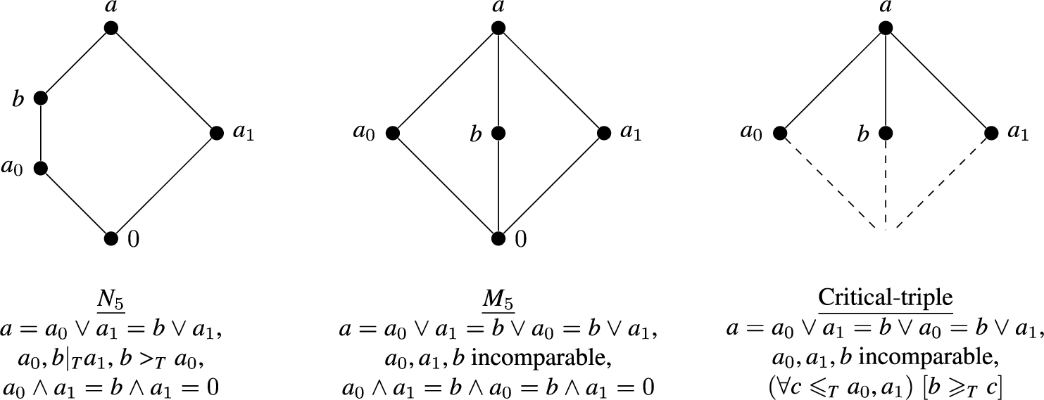
One of the major themes in the study of the c.e. degrees is to identify the lattices that can be embedded below $0^{'}$ and to characterize the degrees below which one can embed a given lattice. It has been known for some time that all distributive lattices, which are lattices that do not contain $N_{5}$ or $M_{5}$ (Fig. 1) as sub-lattices, can be bounded below any c.e. degree d [12]. As for the two basic non-distributive lattices, it is known that being able to bound $N_{5}$ with top element d is exactly the same as being non-contiguous [7]. Little was known about $M_{5}$ until 2020, when it was finally shown that d bounds $M_{5}$ if and only if d is “sufficiently fickle” [2] – some set in d needs to have a computable-approximation of fickleness $⩾ ω^{ω}$ in order for d to bound $M_{5}$ . We formally define what it means for a set or degree to have fickleness α1

¹
Downey and Greenberg used the term “properly totally α-computably approximable” to refer to sets or degrees with fickleness α. To be less verbose, we refer to this property as being α-fickle. Also, we use the term $⩽ α$ -fickle to refer to the property of being totally α-computably approximable.

in Section 4.

In a similar vein, to embed the critical triple, which is a structure resembling $M_{5}$ but with fewer meet conditions (Fig. 1), a c.e. degree only needs to have fickleness $> ω$ to succeed [3]. Therefore a degree’s ability to embed certain lattices is highly dependent on the degree’s fickleness. This connection follows from the techniques used to construct a c.e. degree that embeds a specific lattice, which involve prioritizing the requirements for embeddability and satisfying them in turn. A more fickle degree is more likely to permit requirements to be satisfied, increasing the chances of a successful construction.

Motivated by how fickleness aids embeddability, Downey and Greenberg [2] defined a hierarchy of c.e. degrees, placing degrees that are more fickle higher up the hierarchy. It turns out that c.e. degrees with “reasonable” fickleness are low² [2]. Lying at the bottom level of the hierarchy are the least fickle degrees, and of these degrees those that are “uniformly fickle” are exactly the array computable ones [2].

Figure 1.

Lattices $N_{5}$ , $M_{5}$ , and critical triple structure. The critical triple is similar to $M_{5}$ but does not require meets $a_{0} \land a_{1}$ , $b \land a_{0}$ , or $b \land a_{1}$ to exist.

Our work is based on this recent work of fickleness characterizing embeddability strength. Given that nonlowness is another measure of degree strength and that all α-fickle degrees are low², we explore how lowness and nonlowness sits within the fickleness hierarchy. We expect nonlow degrees to compute more degrees than low ones, but does that necessarily imply nonlows embed more types of lattices? This statement is believed to be false, for Downey and Greenberg [2] claimed there are lows and nonlows on every level of the fickleness hierarchy. But we are not aware of any formal proof in literature, and provide one here.

Given an arbitrary “reasonable” ordinal α, we construct low and nonlow c.e. sets whose degrees d are α-fickle. We begin by building a nonlow c.e. set whose degree’s fickleness is ω, the lowest non-trivial level. Our construction distributes injury from the nonlow requirements uniformly across the sets in the degree, making our degree uniformly ω-fickle, or equivalently, array computable. Therefore we have explicitly built a nonlow array computable c.e. set, which are also sets whose proof of existence have always been indirect .2

First, construct an array computable, 1-topped, and incomplete c.e. set, then use the fact that every array computable and 1-topped degree is either incomplete or nonlow ${low}_{2}$ [6]. Alternatively, construct a nonlow c.e. degree that contains only a single W-degree and whose elements are all mitotic, then use the fact that every array noncomputable c.e. degree must contain a c.e. set that is non-W-mitotic [1].

Next, given an arbitrary $α > ω$ , we injure sets in d exactly “α-times more” to raise the fickleness of d up to α. To build a low set of fickleness α, we “simplify” the construction given by Downey and Greenberg ([2], Lemma III.2.1), where the authors constructed a c.e. set at the α-level of the hierarchy. The authors used a tree in the construction so the constructed set was not necessarily low. By tracking injury more carefully, we managed to avoid using a tree, ensuring lowness. Our construction is also uniform enough, making the constructed degrees not just α-fickle but uniformly α-fickle.

2. Array computability

The least non-trivial level of fickleness of a c.e. degree is ω [2], and the array computable degrees are exactly the $⩽ ω$ -fickle degrees whose fickleness are uniform in the following sense:

Definition 2.1.
A c.e. degree d is array computable [5] if there exists a total computable function $m (x) : ω \to ω$ known as the mind-change function such that every $A \in d$ has a uniformly computable approximation $a (x, s) \equiv_{T} \emptyset$ where for all $x \in ω$ ,
$A (x) = {lim}_{s} a (x, s)$ , and

$(\exists^{< m (x)} s) [a (x, s) \neq a (x, s + 1)]$ .

Array computability was introduced by Downey, Jockusch, and Stob [4], after observing how sufficient fickleness was enough to satisfy many commonly encountered embeddability requirements. Array computability turned out to characterize the c.e. degrees with a strong minimal cover [11], showing again the connection between fickleness and lattice structure.

We shall give a direct construction of a nonlow and array computable c.e. set. Our construction uses the usual tree framework to handle infinite injury from the various requirements. Refer to [13] Chapter 14 for priority constructions using trees. First we introduce common construction terminologies in the following Section 2.1.
2.1. Tree constructions

We mainly follow terminology from [2] Chapter 1.1. Often in the construction we say that we pick a large number as a use or a follower. Large refers to the first number greater than any number that has ever been seen or used up to the point of construction. Requirements are ordered $R_{0} < R_{1} < R_{2} < \dots$ , with smaller requirements having higher priority than larger ones.

Trees provide an intuitive framework for infinite injury constructions. Such constructions begin by fixing an ordering of the requirements $R_{0} < R_{1} < \dots$ , where each requirement has exactly one true outcome from an ordered and computable set $outcomes = {o_{0} < o_{1} < o_{2} < \dots}$ , with smaller outcomes having higher priority. The tree of construction is $\begin{matrix} Λ = {outcomes}^{< ω} . \end{matrix}$

At each stage s of the construction, we guess the outcomes of an initial segment of the requirements to get a node $δ_{s} \in Λ$ of outcomes. Given $s \in ω$ and $δ \in Λ$ , if $δ ⪯ δ_{s}$ , we say stage s is an δ-stage, or δ is accessible at stage s. Given $δ, δ^{'} \in Λ$ , we say δ lies to the left of $δ^{'}$ , written $δ <_{L} δ^{'}$ , to mean $\begin{matrix} δ <_{L} δ^{'} ⟺ (\exists η \in Λ, o_{0} < o_{1} \in outcomes) [η^{⌢} o_{0} ⪯ δ and η^{⌢} o_{1} ⪯ δ^{'}] . \end{matrix}$

A node $δ \in Λ$ is said to lie on the true path of outcomes iff δ is accessed infinitely often but any node to the left of δ is only accessed finitely often. Formally, $\begin{matrix} δ lies on true path of outcomes ⟺ (\exists^{\infty} s) [δ ⪯ δ_{s} and (\forall δ^{'} <_{L} δ) [| {t : δ^{'} ⪯ δ_{t}} | < ω]] . \end{matrix}$

Note that from this definition, the set of nodes that lie on the true path must form a chain. We define the true path of outcomes $δ_{ω}$ as the union of this chain $\begin{matrix} δ_{ω} : = \cup {δ \in Λ : δ lies on the true path of outcomes}, \end{matrix}$ and write $δ ≺ δ_{ω}$ to mean that δ lies on this true path. Often in tree constructions we want to show that $| δ_{ω} | = ω$ . Node $δ \in Λ$ is said to be of higher priority than $δ^{'} \in Λ$ if $δ <_{L} δ^{'}$ or $δ ≺ δ^{'}$ .

3. Nonlow, array computable c.e. degree

Theorem 3.1.
There exists a nonlow, array computable c.e. set A.

To make A nonlow, fix a partial computable enumeration of the computable functions ${⟨ {⟨ ψ (y, s) ⟩}_{s} ⟩}_{ψ}$ and construct functional Γ such that $Γ (A)$ is c.e. in A and satisfies positive requirements: $\begin{matrix} P_{ψ} : (\forall y) [lim_{s} ψ (y, s) exists] ⟹ (\exists y) [χ_{Γ (A)} (y) \neq lim_{s} ψ (y, s)] . \end{matrix}$

To see how $P = P_{ψ}$ gives nonlowness, note that $Γ (A)$ is $Σ_{1}$ in A and therefore computable by $K^{A}$ . Also, the limits $ψ (y) : = {lim}_{s} ψ (y, s)$ , when they exist, enumerate all the $Δ_{2}^{0}$ functions by Shoenfield’s limit lemma. Thus the P requirements ensure no $Δ_{2}^{0}$ function computes $K^{A}$ , making A nonlow.

The P-strategy is like the usual diagonalization strategy, where we pick large uses to enumerate into A to diagonalize $χ_{Γ (A)} (y)$ out of the $ψ (y)$ functions. But because $Γ (A)$ only needs to be c.e. in A and not computable in A, we can delay picking P’s use until higher priority negative requirements $N < P$ have settled sufficiently so as to avoid injuring these N too often.

$P = P_{ψ}$ -strategy:

Setup: Initialize P by cancelling all previous followers of P, if any. Pick a large follower y for P.

Await permission to pick use: Wait for $ψ (y) = 0$ and for all higher priority negative requirements to permit P to pick a use. We elaborate on this permission later. If permission is granted choose a large use u and declare $Γ (A ↾ u, y) [s] ↓$ , where s is the current stage. We say that P acts via picking use.

Enumerate use: Wait for $ψ (y) = 1$ . We say that P wants to act via enumeration. Enumerate u into A and return to the previous state of awaiting permission to pick use.

Observe that if $ψ (y)$ does not exist then P may act infinitely often, enumerating infinitely many elements into A. Therefore P requirements potentially inflict infinite injury, which may cause problems for lower priority negative sub-requirements that can only tolerate finite injury. We circumvent this issue using the usual tree construction, where lower priority requirements play different strategies depending on whether P has finitary outcome $fin$ or infinitary outcome ∞. Letting ρ be a node in the tree working for P, we believe that ρ has outcome ∞ at ρ-stage s iff

either $ψ (y, s) = 0$ and ρ does not have a use at stage s,

or $ψ (y, s) = 1$ and ρ has a use at stage s.

Otherwise we believe ρ has finitary outcome $fin$ . If ρ’s outcome is $fin$ then a lower priority negative node $η ⪰ ρ^{⌢} fin$ will wait for ρ to finish acting before believing computations. On the other hand if $η ⪰ ρ^{⌢} \infty$ then η will delay believing computations until the use picked by ρ is too large to injure η substantially. We elaborate on this η-strategy after introducing the negative requirements which gives array computability: We want to construct a total computable mind-change function $m (x) : ω \to ω$ such that for all Φ, $\begin{matrix} N_{Φ} : (\forall x) (\exists^{< m (x)} s) [Φ (A, x) [s] \neq Φ (A, x) [s + 1]] . \end{matrix}$

Let η be a node in the tree that works for $N = N_{Φ}$ . To meet η, given $x \in ω$ wait for $Φ ↾ x ↓$ and protect $Φ (x)$ against injuries from positive nodes ρ. As just mentioned, if $ρ ⪯ η$ then the tree construction helps ρ reduce injury on $Φ (x)$ as follows: A ρ-node with use u at stage s is said to threaten $Φ (x)$ if $u < use (Φ, x) [s]$ or $Φ (x) ↑ [s]$ . Let δ be an arbitrary node comparable with $η^{⌢} \infty$ . $Φ (x)$ is said to be δ-correct at stage s iff $Φ (x) ↓ [s]$ and no $ρ^{⌢} \infty ⪯ δ$ threatens $Φ (x)$ at stage s. We believe $Φ (x)$ to be correct at stage s if $Φ (x)$ is η-correct at stage s. We shall see that this strategy of delaying believing computations until they are η-correct is enough to protect $Φ (x)$ against injury from higher priority $ρ ≺ η$ .

Protecting against lower priority $ρ ⪰ η$ requires a different strategy because η does not know if ρ has finitary or infinitary outcome, and therefore cannot wait for the use of ρ to get sufficiently large or risk waiting forever. We want a strategy that ensures computation $Φ (x)$ changes less than $m (x)$ -times. Now ρ knows if $Φ (A)$ is total and can therefore reduce injury on η by delaying picking uses until enough $Φ (x)$ computations are believed to be $ρ^{⌢} \infty$ -correct. We formalize later how many x is enough.

To guess if $Φ (A)$ is total we use the usual method involving η-expansionary stages: Define the length of η at stage s as: $\begin{matrix} length (η) [s] : = max {x ⩽ s : Φ ↾ x ↓ is η -correct at stage s} . \end{matrix}$ We say s is an η-expansionary stage iff $\begin{matrix} length (η) [s] > max {length (η) [s^{'}] : s^{'} < s is an η -stage} . \end{matrix}$ At η-stage s the outcome of η is believed to be ∞ if s is η-expansionary and believed to be $fin$ otherwise. Since each requirement in this construction has possible outcomes ${\infty < fin}$ , our tree of construction will be $\begin{matrix} Λ : = {\infty, fin}^{< ω} . \end{matrix}$

Now if $ρ ⪰ η^{⌢} \infty$ and ρ wants to pick a use, a naive strategy is to wait for $Φ (x)$ to be ρ-correct for all $x ⩽ length (η)$ . But such a strategy may result in ρ never being permitted to pick a use: Consider the situation where $η^{⌢} \infty ⪯ ρ^{' ⌢} \infty ⪯ ρ$ , and where ρ is not permitted to pick a use because $ρ^{'}$ is threatening $Φ (l - 1)$ , where $l = length (η)$ . The use of $ρ^{'}$ will eventually be enumerated into A, but at $ρ^{⌢} fin$ -stages $ρ^{'}$ may pick a new use which then threatens $Φ (l)$ at the next $ρ^{⌢} \infty$ -stage, denying ρ permission to pick a use again.

Therefore we need a strategy where ρ will be allowed to pick a use by all large enough x even if $Φ (x)$ is not necessarily $ρ^{⌢} \infty$ -correct. We introduce a quota system to decide which x is large enough. We fix a computable function of finite sets $quota (x)$ which contains positive nodes allowed by x, and ensure that
$quota (x) \subseteq quota (x + 1)$ ,

and $⋃_{x \in ω} quota (x) = {ρ : ρ \in Λ}$
so that all ρ eventually get infinitely opportunities to pick uses. To these ends, we let $\begin{array}{l} (1) & quota (x) = {δ \in Λ : | δ | < x and δ works for a positive requirement} . \end{array}$

To limit the injury on $Φ (x)$ , we allow each ρ to pick a use the incorrect way no more than once:

$η = N_{Φ}$ -strategy:

Initialize: Discard all previous tracking of injuries on $Φ (x)$ .

Maintain: Wait for stage to be η-expansionary. For each $x < length (η)$ keep track of injury of $Φ (x)$ . If $ρ ⪰ η^{⌢} \infty$ wants to pick a new use, permit ρ to do so if
$length (η) > {argmin}_{z} {ρ \in quota (z)}$ ,

and for all $x < length (η)$

either $Φ (x)$ is $ρ^{⌢} \infty$ -correct,

or $ρ \in quota (x)$ and there was no previous stage where ρ picked a use when $Φ (x)$ was not $ρ^{⌢} \infty$ -correct.
Nodes that want to act via enumeration are always granted permission. Return to the beginning of the maintenance state.

ρ is permitted to act at a ρ-stage s iff every η where $η^{⌢} \infty ⪯ ρ$ permits ρ to do so. Condition (2a) of the η-strategy is a necessary detail that delays the picking of uses for nodes outside x’s quota until $x < length (η)$ . The delay prevent these outside nodes from threatening and injuring $Φ (x)$ , as we shall prove in Lemma 3.4. Note that condition (2a) will eventually be satisfied because $⋃_{x \in ω} quota (x)$ covers all positive nodes in Λ. We also prove in the lemma that we can bound injury on $Φ (x)$ as a computable function of $quota (x)$ .

Construction. Stage 0: Initialize all nodes in Λ.

Stage $s + 1$ : Let $δ_{s} \in {\infty, fin}^{s}$ be the node guessing the outcomes of the first s requirements. If any $ρ ⪯ δ_{s}$ has not been accessed since it was last initialized, set up node ρ. Initialize all nodes to the right of $δ_{s}$ . Let $\begin{array}{l} Θ_{s} : = {ρ : ρ^{⌢} \infty ⪯ δ_{s} and ρ is permitted to act}, \\ ρ_{s} : = \underset{ρ \in Θ_{s}}{argmin} {⟨ ρ, k ⟩ : ρ has acted k -times so far} . \end{array}$

If $ρ_{s}$ exists let $ρ_{s}$ act. Go to next stage.
Lemma 3.2.
$| δ_{ω} | = ω$ .
Proof.
Follows immediately from the facts that $| δ_{s} |$ is increasing in s and that Λ is finitely branching. □
Lemma 3.3.
If $ρ ≺ δ_{ω}$ and ρ works for $P_{ψ}$ , then
ρ eventually stops being initialized and therefore has a final follower y,

if $ρ^{⌢} fin ≺ δ_{ω}$ , then if ${lim}_{s} ψ (y, s)$ exists the limit will not equal $χ_{Γ (A)} (y)$ ,

if $ρ^{⌢} \infty ≺ δ_{ω}$ , then ρ will act infinitely often, which implies that ${lim}_{s} ψ (y_{ρ}, s)$ does not exist.
Therefore $P_{ψ}$ is satisfied.
Proof.
Wait for all $δ ≺ ρ$ to stop being initialized and for all $δ <_{L} ρ$ to stop being visited. Such a stage exists by induction hypothesis. Then ρ will never be initialized, which proves the first part of the lemma. The second part holds because ρ will choose outcome ∞ the moment $ψ (y, s)$ agrees with $χ_{Γ (A)} (y)$ .

For the third part, assume ρ has a final follower y and outcome ∞. Assume for contradiction that ρ only acts $(k - 1)$ -times during the construction. Wait for these $(k - 1)$ -actions to occur. For each $⟨ σ, k^{'} ⟩ < ⟨ ρ, k ⟩$ where σ is a positive node wait for σ to act $k^{'}$ -times or to stop wanting to act forever. Then our construction ensures that ρ will always have the highest priority to act. Since permission is always granted for enumerating uses, it must be that ρ wants to pick a use but was always denied permission.

Let $l = {argmin}_{z} {ρ \in quota (z)}$ . For each η where $η^{⌢} \infty ⪯ ρ$ let $η = N_{Φ}$ and wait for the first $ρ^{⌢} \infty$ -stage after which computations $Φ ↾ (l + 1)$ have settled, say at stage s; such a stage exists from induction hypothesis. Then for each such η wait for $Φ ↾ (length (η) [s])$ to settle, say at stage $s^{'} ⩾ s$ . Then condition (2a) of the η-strategy will always be satisfied.

If $x ⩽ max {length (η) [s], l}$ , then $Φ (x)$ must forever be $ρ^{⌢} \infty$ -correct: Otherwise there exists some $ρ^{'}$ with $ρ^{' ⌢} \infty ⪯ ρ$ that threatens $Φ (x)$ with use u. But by induction hypothesis u will eventually be enumerated into A, contracting that $Φ (x)$ has settled. Therefore x would satisfy condition (2(b)i) of the η-strategy.

On the other hand, if $x > max {length (η) [s], l}$ , then $ρ \in quota (x)$ , implying that ρ is allowed by $Φ (x)$ to pick a use non ρ-correctly once. This allowance is not exhausted because $x < length (η)$ for the first time only after ρ stopped picking uses. Therefore x would satisfy condition (2(b)ii) of the η-strategy.

So after stage $s^{'}$ , ρ must be permitted to pick a use, a contradiction. □
Lemma 3.4.
If $η ≺ δ_{ω}$ and η works for $N_{Φ}$ , then
η eventually stops being initialized,

if $η^{⌢} fin ≺ δ_{ω}$ , then $Φ (A)$ is not total,

if $η^{⌢} \infty ≺ δ_{ω}$ and $Φ (A)$ is total, then for all x injury on $Φ (x)$ is bounded by $2^{2 x^{2}}$ .
Thus letting $m (x) = 2^{2 x^{2}}$ , by all parts of the lemma, $N_{Φ}$ is satisfied.
Proof.
For the first part of the lemma wait for all $δ ≺ η$ to stop being initialized, which will eventually happen from induction hypothesis. Wait for all $δ <_{L} η$ to stop being visited. Then η will never be initialized again. For the second part, assume for contradiction Φ is total yet there is a smallest x such that $Φ (x)$ is never η-correct. Wait for $Φ ↾ (x + 1) ↓$ to settle. There must be some $ρ^{⌢} \infty ⪯ η$ that threatens $Φ (x)$ via some use u. By induction hypothesis with Lemma (3.3.3), u must eventually be enumerated into A, contradicting the fact that $Φ (x)$ has settled.

The third part of the lemma is the heart of the argument on why the construction works. Wait for $x < length (η)$ for the first time at an $η^{⌢} \infty$ -stage s after η stops being initialized. As explained in the η-strategy, positive nodes that threaten $Φ (x)$ at stage s must lie in $quota (x)$ . Note that nodes that injure $Φ (x)$ must threaten $Φ (x)$ at some $η^{⌢} \infty$ -stage before inflicting the injury. Given $ρ \in Λ$ we now bound the injury that ρ can inflict on $Φ (x)$ . Unless specified always assume we are working in $η^{⌢} \infty$ -stages after stage s.

Case $ρ <_{L} η$ : Injury is 0 because such ρ are never visited again after η stops being initialized.

Case $ρ >_{L} η$ : Injury is 0 because such ρ are initialized at $η^{⌢} \infty$ -stages and can therefore never threaten $Φ (x)$ .

Case $ρ ≺ η$ : Injury is 0 because by η-correctness of $Φ (x)$ at $η^{⌢} \infty$ -stages such ρ cannot threaten $Φ (x)$ .

Case $ρ \notin quota (x)$ : Injury is 0. Assume for contradiction there is a first such ρ that threatens $Φ (x)$ , say at stage $s_{1}$ via use u, which was picked at stage $s_{0} < s_{1}$ . Between stages $s_{0}$ and $s_{1}$ there must have been an earliest stage where $Φ (x)$ was injured by some other $ρ^{'}$ that threatened $Φ (x)$ at stage $s_{0}$ . We say that $ρ^{'}$ caused ρ to threaten $Φ (x)$ via use u. Now $ρ^{'}$ must lie in $quota (x)$ by choice of ρ being the first. Therefore $ρ^{'} ⋡ ρ$ because such nodes lie outside $quota (x)$ by the fact that $quota (x)$ is closed under initial segments as defined in Equation (1). Also, $ρ^{'} ⊀ ρ$ otherwise ρ would not have picked a use at stage $s_{0}$ given that $Φ (x)$ would not have been ρ-correct. Furthermore, $ρ^{'} ≮_{L} ρ$ otherwise u would be cancelled when $ρ^{'}$ injured $Φ (x)$ . Finally, $ρ^{'} ≯_{L} ρ$ otherwise at stage $s_{0}$ , ρ would have initialized $ρ^{'}$ and its threatening use. So $ρ^{'}$ cannot exist.

Case $ρ \in quota (x)$ and $ρ ⪰ η^{⌢} \infty$ : ρ might have picked its first use at a non ρ-correct stage. Wait for this use to be enumerated, injuring $Φ (x)$ once. Assume some $ρ^{'}$ causes ρ to threaten $Φ (x)$ again. Then because ρ can only pick uses at ρ-correct stages from now on, we can use the same arguments as in the previous case to show that $ρ^{'} ⋠ ρ$ , $ρ^{'} ≮_{L} ρ$ , or $ρ^{'} ≯_{L} ρ$ . So it must be that $ρ^{'} ≻ ρ$ , and from the previous case we know $ρ^{'}$ must also lie in $quota (x)$ , giving the inductive relation: $\begin{array}{l} causeThreaten (ρ) : = & {ρ^{'} : ρ^{'} causes ρ to threaten Φ (x)} \\ (2) & \subseteq {ρ^{'} ≻ ρ : ρ^{'} \in quota (x)} . \end{array}$

We prove by induction on $x - | ρ |$ that ρ injures $Φ (x)$ no more than $2^{2 {(x - | ρ |)}^{2}}$ -times: The base case where $x - | ρ | = 0$ follows from the fact that such ρ do not lie in $quota (x) \subseteq 2^{< x}$ and therefore does not injure $Φ (x)$ as argued earlier. For the inductive step assume the proposition holds for all nodes in $quota (x)$ with length $> | ρ |$ . Now modulo one possible initial injury described earlier, every subsequent injury inflicted by ρ is caused by an injury inflicted by some $ρ^{'} \in causeThreaten (ρ)$ , and each such $ρ^{'}$ inflicts no more than $2^{2 {(x - | ρ | - 1)}^{2}}$ -injuries by induction hypothesis, therefore $\begin{array}{l} Injury from ρ & ⩽ 2^{2 {(x - | ρ | - 1)}^{2}} \cdot | causeThreaten (ρ) | + 1 & (induction hypothesis) \\ ⩽ 2^{2 {(x - | ρ | - 1)}^{2}} \cdot | {ρ^{'} ≻ ρ : ρ^{'} \in quota (x)} | + 1 & (from Equation (2)) \\ ⩽ 2^{2 {(x - | ρ | - 1)}^{2}} \cdot 2^{x - | ρ |} + 1 & (∵ quota (x) \subseteq 2^{< x}) \\ = 2^{2 {(x - | ρ |)}^{2} - 3 (x - | ρ |) + 2} + 1 \\ ⩽ 2^{2 {(x - | ρ |)}^{2} - 3 (x - | ρ |) + 2} + 2^{2 {(x - | ρ |)}^{2} - 3 (x - | ρ |) + 2} & (∵ the exponent > 0) \\ = 2^{2 {(x - | ρ |)}^{2} - 3 (x - | ρ |) + 3} \\ (3) & ⩽ 2^{2 {(x - | ρ |)}^{2}} . & (∵ x - | ρ | ⩾ 1 after base case) \end{array}$

The inductive step applies until $| ρ | = 1$ . To bound total injury on $Φ (x)$ , apply the inductive step one last time: $\begin{array}{l} (4) & Total injury on Φ (x) ⩽ 2^{2 x^{2}} . \end{array}$ □

Lemmas 3.3 and 3.4 together give: Corollary 3.5.
A is nonlow and array-computable.

4. Defining α-fickle, uniformly α-fickle degrees

Given a “reasonable” ordinal α, in Section 5 we build a low c.e. set whose degree is α-fickle, then show in Section 6 that the constructed set can be made to be uniformly α-fickle. But first we formalize what it means for a c.e. degree to be α-fickle and what it means for α to be reasonable.

By Shoenfield’s Limit Lemma, every $Δ_{2}^{0}$ set A has a computable-approximation $a (x, s) : ω^{2} \to ω$ such that for all $x, s \in ω$ $\begin{matrix} A (x) = lim_{s} a (x, s) . \end{matrix}$

To measure how fickle A is, we want to keep track of how often $a (x, -)$ changes its mind. This idea was formalized as follows:

Definition 4.1 ([8–10]).

Let $R = (R, <_{R})$ be a computable well-ordering (both R and $<_{R}$ are computable), and let A be a $Δ_{2}^{0}$ set. An $R$ -computable-approximation ( $R$ -c.a.) of A is a computable-approximation $a (x, s) : ω^{2} \to ω$ of A together with a computable mind-change function $m (x, s) : ω^{2} \to R$ such that for all x and s:

$m (x, s + 1) ⩽_{R} m (x, s)$

if $a (x, s + 1) \neq a (x, s)$ , then $m (x, s + 1) <_{R} m (x, s)$ .

For the notion of fickleness to be independent from the $R$ used, we restrict the ordinals considered to $\begin{matrix} α < ϵ_{0} : = sup {ω, ω^{ω}, ω^{ω^{ω}}, \dots}, \end{matrix}$ and require that the computable approximations $R$ considered be canonical:

Definition 4.2 ([2] II.D2.2).

Let $R$ be a computable well-ordering with order type α. Let ${nf}_{R} : ω \to {(ω^{2})}^{< ω}$ denote the function that takes each ordinal below α to its Cantor-normal form, i.e. $\forall z \in R$ $\begin{matrix} {nf}_{R} (z) = ⟨ ⟨ z_{0}, n_{0} ⟩, \dots, ⟨ z_{i}, n_{i} ⟩ ⟩, \end{matrix}$ where $z_{j} \in R$ , $| z_{0} | > \dots > | z_{i} |$ , $n_{j} \in ω - {0}$ , and $\begin{matrix} | z | = ω^{| z_{0} |} \cdot n_{0} + \dots + ω^{| z_{i} |} \cdot n_{i} \end{matrix}$ gives the unique Cantor-normal form of $| z |$ . If ${nf}_{R}$ is computable, we say that $R$ is canonical.

Definition 4.3 ([2] II.D2.9, III.D1, III.L1.1).

Let $A, d \in Δ_{2}^{0}$ .

A is $⩽ α$ -fickle3

³
$⩽ α$ -fickleness of a set was originally introduced in [2] as being α-computably-approximable.

if A has a canonical

R

-c.a. of order type α.

A is α-fickle if α is the smallest ordinal such that A is $⩽ α$ -fickle.

d is $⩽ α$ -fickle4

⁴

$⩽ α$ -fickleness of a degree was originally introduced in [2] as being totally α-computably-approximable.

if every set in d is

⩽ α

-fickle.

d is α-fickle5

⁵

α-fickleness of a degree was originally introduced in [2] as being properly totally α-computably-approximable.

if α is the smallest ordinal such that d is

⩽ α

-fickle.

d is uniformly α-fickle if d is α-fickle and there is a single mind-change function that witnesses $⩽ α$ -fickleness of every set in d.

Note that if A is α-fickle, even though α may be infinite, each $A (x)$ only changes its mind finitely often from Definition 4.1 and the fact that there are no infinite descending sequences of ordinals. Therefore when we construct a degree later with $⩾ ω$ -fickleness, the fickleness requirements considered inflict only finite injury.

By canonicalness of $R$ the fickleness hierarchy obtained gives meaningful lattice embeddability results – the $> ω$ -fickle degrees are exactly those that can bound the critical-triple [3], and the degrees that contain $⩾ ω^{ω}$ -fickle sets are exactly those that can bound $M_{5}$ [2]. Also, if $α ⩽ ϵ_{0}$ , a degree’s fickleness will not depend on the $R$ picked ([2] II.P2.3, P2.8), hence in Definition 4.3 the choice of $R$ would not matter. Restricting ourselves to these reasonably small ordinals is enough for now since the embeddability results discussed have levels $ω, ω^{ω} < ϵ_{0}$ . The fickleness hierarchy turns out to collapse exactly to the powers of ω:

Theorem 4.4 ([2] III.L2.1,2).

Let $α ⩽ ϵ_{0}$ . α-fickle degrees exist if and only if α is a power of ω.

The key ingredient that makes Fact 4.4 hold is:

Fact 4.5 (Folklore).

An ordinal α is closed under ordinal addition if and only if α is a power of ω.

Consider how we can construct a set A whose degree is α-fickle. To avoid being $< α$ -fickle, A needs to compute some $Δ (A)$ that diagonalizes out of all the $< α$ -fickle functions. This positive requirement calls for an uniform enumeration of these functions, which we can get from the following fact:

Lemma 4.6 ([2] II.L2.6).

Let $α ⩽ ϵ_{0}$ . We can uniformly enumerate the $< α$ -fickle functions: There exists a canonical $R$ of order type α, a computable function $g (e) : ω \to R$ known as the bounding function, and uniformly computable functions $f^{e} (x, s) : ω^{3} \to ω$ and $m^{e} (x, s) : ω^{3} \to R$ known as the computable-approximation functions, such that ${⟨ f^{e} (x, s), m^{e} (x, s) ⟩}_{s}$ is a $g (e)$ -computable-approximation of $f^{e} (x) : = {lim}_{s} f^{e} (x, s)$ , and ${⟨ f^{e} ⟩}_{e \in ω}$ enumerates the $< α$ -fickle functions.

Now when diagonalizing $Δ (A)$ out of a β-fickle function $f^{e}$ , where $β < α$ , β-many elements 6

⁶
The number of elements is finite, but the elements can only be indexed canonically by a possibly infinite ordinal β.

may be enumerated into A. At the same time, to bound

\deg (A)

’s fickleness

⩽ α

, if

Φ (A)

is total, then for all

x \in ω

Φ (A, x)

cannot change its mind more than α-times. Yet

Φ (A, x)

must tolerate β-injury from each of its higher priority positive requirements. There are only finitely many such requirements, so the total injury on

Φ (A, x)

will turn out to be a finite sum of ordinals

β < α

. This sum can be bounded below α if and only if α is closed under ordinal addition, which is why Fact 4.5 is crucial for a successful construction of an α-fickle degree, evidenced in Theorem 4.4.

The α-fickle degrees turn out to be low², which makes it meaningful to ask if low degrees or nonlow degrees exist at every level of the hierarchy. Lemma 4.7 ([2] III.T1.2).

Let $α ⩽ ϵ_{0}$ . If d is α-fickle then d is low ² .

5. Low, α-fickle C.e. degree

Theorem 5.1.
Let $α ⩽ ϵ_{0}$ be a power of ω. Then there exists a c.e. set A that is low and whose degree d is α-fickle.

A construction outline was provided by Downey and Greenberg ([2] III.L2.2), where the authors built a c.e. set of α-fickle degree using a tree in their proof. Because lowness generally doesn’t mix on trees, it is not clear if the constructed set is low. We shall use the same requirements to construct A at the α-level, but count injury more carefully to avoid using a tree, thus ensuring the lowness. We further show in Lemma 6.1 that if we order our requirements carefully we can make A uniformly α-fickle.

We use the standard finite injury construction and bound the fickleness of each $Φ (A, x)$ below α for all $Φ, x$ . Fix a uniformly computable series of functions ${⟨ {⟨ f (y) [s] ⟩}_{y, s} ⟩}_{f}$ from Lemma 4.6 that enumerates all the $< α$ -fickle functions. Note that for every f and y, $f (y) : = {lim}_{s} f (y) [s]$ exists. Also, fix a computable bounding function $g (f) : ω \to α$ from Lemma 4.6 which tells us that $f (y)$ is $g (f)$ -fickle.

To make d not $< α$ -fickle, we build an A-computable total function $Δ (A)$ that diagonalizes out of all the $< α$ -fickle functions f. Therefore for all f we satisfy the positive requirement: $\begin{matrix} Q_{f} : (\exists y) [Δ (A, y) \neq f (y)] . \end{matrix}$

The $Q = Q_{f}$ -strategy is like a typical diagonalization strategy, where we pick a large follower y and large use u for y, and diagonalize $Δ (A, y)$ out of $f (y)$ by enumerating u into A. But unlike the P-strategy of Theorem 3.1, because we need $Δ (A)$ to be total and not just c.e. in A, we cannot delay picking uses u for y; once y has been picked we need $Δ (A ↾ u, y) ↓$ at every stage of the construction.

$Q = Q_{f}$ -strategy:

Setup: Initialize Q by stopping all action for the previous follower of Q, if it had one. Pick a large follower y and large use u and set $Δ (A ↾ u, y) = 1 - f (y) [s]$ .

Await equality: Wait for $Δ (y) = f (y)$ . We say that Q wants to act. Initialize all lower priority $Q^{'} > Q$ . If permission is granted by negative requirements enumerate the use into A and pick a new large use u and set $\begin{matrix} Δ (A ↾ u, y) = 1 - f (y) [s] . \end{matrix}$ Return to beginning of this state where we await equality again.

Notice that because ${lim}_{s} f (y) [s]$ exists the injury inflicted by Q requirements is finite. As we shall see, each negative requirement also inflicts only finite injury, hence if we can count injury carefully we will not need a tree in the construction, which turns out to be enough to make the constructed set low.
Remark 5.2.
To make our verification later easier, we shall assume that g has the following properties:
g is non-decreasing

For all f, $g (f) < α$ and is a power of ω.

We can assume the first assumption by thinking of $g (n)$ as $max {g (0), \dots, g (n)}$ . We can assume the second assumption from Theorem 4.4; to make $\deg (A) ⩾ α$ -fickle we only need $Δ (A)$ to diagonalize out of the β-fickle functions for all $β < α$ that are powers of ω. In particular, if $α = ω^{β + 1}$ then we only need to diagonalize out of the $ω^{β}$ -fickle functions, and if $α = ω^{α_{0}}$ for some limit ordinal $α_{0}$ then we only need to diagonalize out of the $ω^{β}$ -fickle functions for all $β < α_{0}$ .

For d to be $⩽ α$ -fickle and low, we construct a total computable mind-change function $m (Φ, x) : ω^{2} \to α$ such that for all Φ and x we satisfy negative requirements $\begin{matrix} N_{Φ, x} : (\exists^{⩽ m (Φ, x)} s) Φ (A, x) [s] \neq Φ (A, x) [s + 1] . \end{matrix}$

To see how these $N = N_{Φ, x}$ requirements make $d ⩽ α$ -fickle, given $Φ (A) \in d$ , $m (Φ, -)$ witnesses that $Φ (A)$ is $⩽ α$ -fickle. To get lowness, we want to $0^{'}$ -computably determine if $Φ (A, Φ) ↓$ . The $N_{Φ, Φ}$ requirements ensure that $Φ (A, Φ)$ either converges or eventually diverges forever. Since the construction will be shown to be finite injury, $0^{'}$ will be able to tell which of the cases is true to determine if $Φ \in {(0^{'})}^{A}$ .

Our strategy for N is to tolerate injury only from higher priority positive requirements $Q < N$ , and for each such Q to tolerate injury only up to the stage where some $Q^{'} < Q$ wants to act. Q-requirements that are no longer tolerated but whose action will injure $Φ (x)$ will be initialized by N. To formalize this strategy, we let N maintain a flag $flag (N) [s] \in ω$ to denote that N will tolerate injury only from positive requirements $Q ⩽ flag (N) [s]$ .

$N = N_{Φ, x}$ -strategy:
Setup. Initialize N by setting its flag to undefined. Letting $| R | \in ω$ denote the priority of a given requirement R, at stage $| N | + 1$ set $flag (N) = N$ .

Maintain. If Q is the highest priority positive requirement that wants to act, update $\begin{matrix} flag (N) [s] = min {Q, flag (N) [s - 1]} . \end{matrix}$ N permits Q to act with use u if
either $Q ⩽ flag (N) [s]$ ,

or $u > use (Φ, x) [s]$ .
Return to the beginning of this maintenance state.
Q is permitted to act at stage s if every $N < s$ permits Q to act at stage s.

Construction. Stage 0: Initialize all requirements.

Stage $s + 1$ : Set up the first s-th requirements if they are not already set up. Let $Q ⩽ s$ be the highest priority positive requirement that wants to act. Go to next stage if Q does not exist. For all $N ⩽ s$ maintain N like described in the N-strategy. Let Q act if permission is granted by all $N ⩽ s$ , otherwise initialize Q. Lemma 5.3.
Q is satisfied.
Proof.
By induction hypothesis we can wait for all $Q^{'} < Q$ to be satisfied at a stage $s_{0} > | Q |$ . If $N ⩽ s_{0}$ , then $N = N_{Φ, x}$ cannot initialize Q more than once: Wait for N to initialize Q again, say at stage $s_{1} ⩾ s_{0}$ ; if this never occurs we are done. Then N’s flag will be set to $⩽ Q$ to prevent any $Q^{'} > Q$ from injuring $Φ (x) ↓ [s_{1}]$ . But all $Q^{'} < Q$ have finished acting, so the only requirement that can injure N is Q. But after stage $s_{1}$ the uses picked by Q will exceed $use (Φ, x) [s_{1}]$ , preventing Q from injuring N. Therefore computation $Φ (x)$ would have settled at stage $s_{1}$ so N can never initialize Q again.

Also, if $N > s_{0}$ , then N can never initialize Q: Such N are setup after stage $s_{0}$ , so their flags at the stage of setup is $⩾ s_{0} > Q$ . This flag never drops below Q because all $Q^{'} < Q$ have stopped wanting to act. Therefore N will always permit Q to act.

Therefore after higher priority positive requirements are satisfied at stage $s_{0}$ , Q will not be initialized more than $s_{0}$ -times. After these initializations the follower y of $Q = Q_{f}$ will be finalized and Q will always be permitted to act otherwise it would be initialized. Then after $f (y)$ has settled Q would act for the last time and be satisfied forever. □
Lemma 5.4.
Given $N = N_{Φ, x}$ , let $\bar{Q} (N) : = max {Q : Q < N}$ . Then N is satisfied if we let $\begin{matrix} m (N) = m (Φ, x) = g (\bar{Q} (N)) \cdot {| \bar{Q} (N) |}^{2} . \end{matrix}$
Proof.
From setup the only Q that can injure N must have higher priority than N. We show that after stage $| N |$ when N is setup, each $Q < N$ will not be initialized more than $| Q |$ -times before becoming no longer tolerated by N: Let $s_{0}$ be the first stage $> | N |$ where some $Q^{'} < Q$ wants to act. If this stage doesn’t exist let $s_{0} = ω$ . We show that between stages N and $s_{0}$ , Q can only be initialized by $N^{'} < Q$ , and no more than once by each such $N^{'}$ : If $N^{'} < Q$ the positive nodes that $N^{'}$ tolerates must be of higher priority than Q. But these nodes do not act before stage $s_{0}$ , implying that up to stage $s_{0}$ the use of the computation of $N^{'}$ increase no more than once, thereby initializing Q no more than once. On the other hand, if $N^{″} > Q$ , then $N^{″}$ is setup with a flag $⩾ Q$ , meaning that $N^{″}$ will tolerate injury from Q until stage $s_{0}$ when some $Q^{'} < Q$ acts, which completes our claim.

Now between consecutive initializations of some $Q = Q_{f}$ , Q cannot inflict more than $g (Q) = g (f)$ -injury on N. Therefore from above argument $\begin{array}{l} Injury on N & ≲ \sum_{Q < N} g (Q) \cdot | Q | \\ ⩽ \sum_{Q < N} g (Q) \cdot | \bar{Q} (N) | & (by definition of \bar{Q} (N)) \\ ⩽ \sum_{Q < N} g (\bar{Q} (N)) \cdot | \bar{Q} (N) |, & (∵ from Remark 5.2, g (Q) is non-decreasing) \\ = g (\bar{Q} (N)) \cdot | \bar{Q} (N) | \cdot \sum_{Q < N} 1 \\ ⩽ g (\bar{Q} (N)) \cdot | \bar{Q} (N) | \cdot | \bar{Q} (N) | & (by definition of \bar{Q} (N)) \\ = g (\bar{Q} (N)) \cdot {| \bar{Q} (N) |}^{2} \\ < α . & (Fact 4.5) \end{array}$

More work needs to be done to ensure that this injury bound $m (N) = g (\bar{Q} (N)) \cdot | \bar{Q} (N) |^{2}$ on N is large enough. The complication arises because ordinal addition is not commutative and not strictly increasing in the left argument (i.e. $α < β$ does not necessarily imply $α + γ < β + γ$ ), which is why the first inequality above was written only as an approximation ≲. We prove in the next lemma that $m (N)$ is large enough. □
Lemma 5.5.
It is enough to set $m (N) = g (\bar{Q} (N)) \cdot | \bar{Q} (N) |^{2}$ to bound on the injury on N.
Proof.
Given N, we want to define a non-increasing mind-change function $o (s) : ω \to m (N) + 1$ that decreases at stages $s ⩾ | N |$ when some $Q ⩽ flag (N) [s]$ injures N. The idea is to keep $o (s)$ in Cantor normal form where ordinal addition is better behaved: At stages $s < | N |$ initialize $o (s) = m (N) = g (\bar{Q} (N)) \cdot | \bar{Q} (N) |^{2}$ . At stage $s ⩾ | N |$ , if no $Q ⩽ flag (N) [s]$ wants to act, let $o (s) = o (s - 1)$ . Otherwise
let $Q_{s}$ be the highest priority positive requirement that wants to act,

let y be the follower of $Q_{s}$ at stage s,

let $\bar{m} (y, t) : ω^{2} \to g (Q_{s})$ be the computable mind-change function that witnesses the $g (Q_{s})$ -fickleness of $Q_{s}$ ,

let $i_{Q_{s}}$ be the number of times that $Q_{s}$ has been initialized since stage $| N |$ , and let
$\begin{matrix} o (s) = g (\bar{Q} (N)) \cdot [| \bar{Q} (N) | \cdot | Q_{s} | + | \bar{Q} (N) | - i_{Q_{s}} - 1] + \bar{m} (y, s - 1) . \end{matrix}$

Note that $o (s)$ is always in Cantor normal form because from Remark 5.2 we can assume that $g (\bar{Q} (N))$ is a power of ω that exceeds $\bar{m} (y)$ . We need to prove that at stages s with action, $o (s) < o (s - 1)$ . One of three things can happen at such a stage:
$flag (N) [s]$ wants to act and is permitted

$flag (N) [s]$ wants to act and is denied

Some $Q ⩽ flag (N) [s]$ wants to act

In case (1) the integer $[| \bar{Q} (N) | \cdot | Q_{s} | + | \bar{Q} (N) | - i_{Q_{s}} - 1]$ remains the same but the ordinal $\bar{m} (y)$ decreases. Then $o (s) < o (s - 1)$ by the fact that ordinal addition is strictly increasing in the right argument. For the remaining two cases the integer decreases and y does not exist so $\bar{m} (y)$ is considered to be 0. Then $o (s) < o (s - 1)$ from the fact that $g (\bar{Q} (N))$ is a power of ω exceeding the previous $\bar{m} (y)$ and from the properties of ordinal addition via Cantor normal form. □

6. Low, uniformly α-fickle C.e. degree

Lemma 6.1.
Let $α ⩽ ϵ_{0}$ be a power of ω. Then there exists a c.e. set A that is low and whose degree d is uniformly α-fickle.
Proof.
In the construction of Theorem 5.1, because $m (Φ, x)$ is total, we can order our $N = N_{Φ, x}$ -requirements carefully so as to make A not just α-fickle but uniformly α-fickle. The idea is to order the requirements such that we pad with enough negative requirements before considering a new positive requirement. Padding works because in Lemma 5.4 we showed that negative requirements are only injured by the positive requirements of higher priority, so padding stops the injury on negative requirements from increasing too quickly. Specifically, we shall prioritize the requirements in Theorem 5.1’s construction as: $\begin{matrix} Q_{0}, N_{0, 0}, Q_{1}, N_{0, 1}, N_{1, 1}, \dots, Q_{i}, N_{0, i}, N_{1, i}, \dots, N_{i, i}, \dots, \end{matrix}$ where $Q_{i} = Q_{f_{i}}$ and $N_{i, x} = N_{Φ_{i}, x}$ . Then given a fixed i, for all $x > i$ , from Lemma 5.4 we get $\bar{Q} (N_{i, x}) = Q_{x}$ , so that $Φ_{i} (x)$ ’s injury is bounded by $\begin{array}{l} m (Φ_{i}, x) & = g (Q_{x}) \cdot | Q_{x} |^{2} \\ = g (Q_{x}) \cdot {(2 + 3 + 4 + \dots + (x + 2))}^{2} \\ = g (Q_{x}) \cdot \frac{{(x + 1)}^{2} {(x + 4)}^{2}}{4} \\ < α . & (Fact 4.5) \end{array}$ Therefore the mind-change function $m (x) = g (Q_{x}) \cdot \frac{{(x + 1)}^{2} {(x + 4)}^{2}}{4}$ witnesses uniform α-fickleness of A. □
7. Nonlow, uniformly α-fickle C.e. degree

Theorem 7.1.

Let $α ⩽ ϵ_{0}$ be a power of ω. Then there exists a nonlow c.e. set A whose degree d is uniformly α-fickle.

The construction is based on the tree framework of Theorem 3.1 but mixed with the Q-strategies of Theorem 5.1. To get nonlowness, we use the same $ρ = P_{ψ}$ -strategy of Theorem 3.1. To get $⩾ α$ -fickleness, we let ξ-nodes on the tree of construction work for the Q-requirements mentioned in Theorem 3.1. The ξ-strategy is exactly the same as the Q-strategy described earlier. ξ-nodes have a single outcome ${fin}$ because ξ-requirements do not inflict infinite injury.7

⁷

Injury by ξ-requirements is finite even though the canonical way of counting the injury would involve ordinals $⩽ α$ that are possibly $⩾ ω$ .

To get uniform $⩽ α$ -fickleness we construct a total computable mind-change function $m (x) : ω \to α$ such that for all Φ we satisfy negative requirements $\begin{matrix} N_{Φ} : (\forall x) (\exists^{m (x)} s) Φ (A, x) [s] \neq Φ (A, x) [s + 1] . \end{matrix}$

We shall see in Lemma 7.5 that it is enough to let $m (x) = g (x) \cdot 2^{4 x^{2}}$ . We let η-nodes on the tree work for $N = N_{Φ}$ -requirements. The η-strategy here is based on the η-strategy of Theorem 3.1, where we allow only positive nodes $ρ, ξ ⪰ η^{⌢} \infty$ in x’s quota to injure $Φ (x)$ . To bound injury from ρ-nodes uniformly below ω, we apply the idea from the earlier η-strategy where each ρ in x’s quota is only allowed to pick uses at non ρ-correct stages at most once. To bound injury from ξ-nodes uniformly below α, we borrow the idea from the N-strategy of Theorem 5.1 where we let $Φ (x)$ tolerate injury from ξ in x’s quota up to the stage s when ξ gets initialized because some higher priority $ξ^{'} ≺ ξ$ or $ξ^{'} <_{L} ξ$ wants to act. At stage s we initialize all positive requirements of lower priority than $ξ^{'}$ and remove these requirements from x’s quota, preventing them from injuring $Φ (x)$ again. Therefore unlike the quota sets of Theorem 3.1, the quota sets here $quota (x) [t]$ changes with time t, and is non-increasing in t. Up to stage s, following ideas from the proof of Lemma 5.4, we shall show in Lemma 7.5 that there is a computable and finite set of negative sub-requirements $Φ^{'} (x^{'})$ that can initialize ξ, and for each such $Φ^{'} (x^{'})$ , there is a computable bound $< ω$ on the number of times $Φ^{'} (x^{'})$ will initialize ξ. Putting these together we get a bound $n < ω$ on the number of times ξ is initialized, and therefore a bound $g (ξ) \cdot n < α$ on the injury inflicted by ξ on $Φ (x)$ .

To guess the outcome of η, we use the same idea involving η-expansionary stages in Theorem 3.1. Note that when we are determining if a given $Φ (x)$ computation is δ-correct, we only need to consider the $ρ ⪯ δ$ requirements and not the ξ requirements, because ξ-requirements are finitary and always believed to have finished acting, if not they would later initialize all nodes of lower priority including δ.

$η = N_{Φ}$ -strategy:

Initialize: Discard all previous tracking of injuries on $Φ (x)$ .

Maintain: Wait for stage to be η-expansionary. For each $x < length (η)$ keep track of injury on $Φ (x)$ . If $ρ ⪰ η^{⌢} \infty$ wants to act, grant permission according to the η-strategy of Theorem 3.1. If $ξ ⪰ η^{⌢} \infty$ wants to act grant permission if for all $x < length (η) [s]$ , either $ξ \in quota (x) [s]$ , or ξ does not threaten $Φ (x)$ . If there is a highest priority ξ that wants to act, regardless of whether permission is granted, for all $x < length (x) [s]$ update $\begin{matrix} quota (x) [s] = quota (x) [s - 1] - {δ : δ is a positive node, and (δ ≻ ξ or δ >_{L} ξ)} . \end{matrix}$ Return to the beginning of the maintenance state.

Positive nodes δ are permitted to act at stage s if every η with $η^{⌢} \infty ⪯ δ$ permits δ to act.

Construction. Stage 0: Initialize all requirements. For all $x \in ω$ initialize $\begin{array}{l} (5) & quota (x) [0] = {δ : δ is a positive node and | δ | < x} . \end{array}$

Stage $s + 1$ : Let $δ_{s}$ be the node of length s in the tree of construction guessing the outcomes of the first s-requirements. If any positive node $δ ⪯ δ_{s}$ has not been accessed since it was last initialized, set up node δ. Initialize all nodes to the right of $δ_{s}$ . Let $\begin{array}{l} Θ_{s} : = & {ρ : ρ^{⌢} \infty ⪯ δ_{s} and ρ is permitted to act} \\ \cup {ξ ⪯ δ_{s} : ξ wants to act at stage s}, \\ σ_{s} : = & {argmin}_{σ \in Θ_{s}} {⟨ σ, k ⟩ : σ has acted k -times so far} . \end{array}$

If $σ_{s}$ does not exists do nothing. If $σ_{s} = ρ$ let ρ act. If $σ_{s} = ξ$ initialize all $δ ≻ ξ$ and $δ >_{L} ξ$ . Maintain all η with $η^{⌢} \infty ⪯ ξ$ , as described in the η-strategy. Let ξ act if permission is granted, otherwise initialize ξ. Go to next stage.

Lemma 7.2.

$| δ_{\infty} | = ω$ .

Proof.

Same as proof of Lemma 3.2. □

Lemma 7.3.

If $ρ ≺ δ_{ω}$ and ρ works for $P_{ψ}$ , then

ρ eventually stops being initialized and therefore has a final follower y,

if $ρ^{⌢} fin ≺ δ_{ω}$ , then if ${lim}_{s} ψ (y, s)$ exists the limit will not equal $χ_{Γ (A)} (y)$ ,

if $ρ^{⌢} \infty ≺ δ_{ω}$ , then ρ will act infinitely often, which implies that ${lim}_{s} ψ (y_{ρ}, s)$ does not exist.

Therefore

P_{ψ}

is satisfied.

Proof.

Exactly the same as the proof of Lemma 3.3. The ξ-nodes do not affect the argument. □

Lemma 7.4.

If $ξ ≺ δ_{ω}$ and ξ works for $Q_{f}$ , then ξ eventually stops being initialized and therefore has a final follower y, and $Δ (A, y) \neq f (y)$ . Therefore $Q_{f}$ is satisfied.

Proof.

Wait for all $δ ≺ ξ$ to stop being initialized, for all $ξ^{'} ≺ ξ$ to stop wanting to act, and for all $δ <_{L} ξ$ to stop being visited, say at stage $s_{0}$ . Then wait for a ξ-stage $s_{1} > s_{0}$ such that for all $η = N_{Φ}$ with $η^{⌢} \infty ⪯ ξ$ , computations $Φ ↾ max (length (η) [s_{0}], | ξ |) ↓$ has settled. $s_{1}$ exists by induction hypothesis. Then ξ can only be initialized because it was denied permission to act. Wait for ξ to be initialized once more, if it ever is. Say the current stage is $s_{2} ⩾ s_{1}$ . Then ξ will never be initialized again, because the higher priority $Φ (x)$ computations have either settled or have quotas $quota (x) [s]$ that contain ξ for all $s ⩾ s_{2}$ . Therefore ξ will have a final follower y.

For the second part of the lemma, assume for contradiction that ξ only acts $(k - 1)$ -times during the construction yet $Δ (A, y) = f (y)$ . Wait for these $(k - 1)$ -actions to occur and for $f (y)$ to settle. For each $⟨ σ, k^{'} ⟩ < ⟨ ρ, k ⟩$ where σ is a positive node wait for σ to act $k^{'}$ -times or to stop wanting to act forever. Then our construction ensures that ξ will always have the highest priority to act. Thus if ξ wants to act permission will always be granted, a contradiction. □

Lemma 7.5.

If $η ≺ δ_{ω}$ and η works for $N_{Φ}$ , then

η eventually stops being initialized,

if $η^{⌢} fin ≺ δ_{ω}$ , then $Φ (A)$ is not total,

if $η^{⌢} \infty ≺ δ_{ω}$ and $Φ (A)$ is total, then for all x injury on $Φ (x)$ is bounded by $g (x) \cdot 2^{4 x^{2}}$ .

Thus letting

m (x) = g (x) \cdot 2^{4 x^{2}}

, by all parts of the lemma,

N_{Φ}

is satisfied.

Proof.

For the first part of the lemma wait for all $δ ≺ η$ to stop being initialized and for all $ξ ≺ η$ to stop wanting to act, which will eventually happen from induction hypothesis. The proof of the second part of the lemma is the same as that in Lemma 3.4.

For the third part of the lemma wait for $x < length (η)$ for the first time at an $η^{⌢} \infty$ -stage $s_{0}$ . We now bound the injury that a given positive node σ can inflict on $Φ (x)$ . By the same argument in Lemma 3.4, if $σ <_{L} η$ or $σ >_{L} η$ then σ cannot threaten or injure $Φ (x)$ . By the same Lemma if $σ = ρ$ and $ρ ≺ η$ then ρ cannot threaten $Φ (x)$ . Also, if $σ = ξ$ and $ξ ≺ η$ , then ξ cannot injure $Φ (x)$ , because if ξ acts then η will be initialized. Therefore nodes that injure $Φ (x)$ must extend $η^{⌢} \infty$ . First let $σ = ξ ⪰ η^{⌢} \infty$ and consider how much injury ξ can inflict:

Case $ξ \notin quota (x) [0]$ : Such ξ are never allowed to injure $Φ (x)$ by construction.

Case $ξ \in quota (x) [0]$ : We can assume $ξ \in quota (x) [s_{0}]$ otherwise the situation reduces to the earlier case. ξ will remain in x’s quota up to a stage when some $ξ^{'} <_{L} ξ$ or $ξ^{'} ≺ ξ$ acts, after which ξ will be removed from the quota and never be allowed to injure $Φ (x)$ again. Let $s_{1} > s_{0}$ be the first ξ-stage where ξ is removed this way, letting $s_{1} = \infty$ if this never occurs. Any injury inflicted by ξ must be inflicted between stages $s_{0}$ and $s_{1}$ . We bound the number of times ξ is initialized between these stages. If ξ is never initialized then the bound is 0. So wait for ξ to be initialized for the first time, say at stage $s^{'} < s_{1}$ . Then all positive nodes $σ ≻ ξ$ and $σ >_{L} ξ$ will be removed from the quotas of all $y ⩽ x$ to prevent them from ever injuring $Φ ↾ (x + 1)$ again. Thus up to stage $s_{1}$ the only positive nodes that can injure $Φ ↾ (x + 1)$ are ξ itself and $ρ ≺ ξ$ nodes. Now if $y ⩾ x$ then ξ will lie in the y’s quota at least up to stage $s_{1}$ , implying that $Φ (y)$ will not initialize ξ. So if ξ is to be initialized the initialization must be due to $Φ (y)$ for some $y < x$ where $ξ \notin quota (y) [s^{'}]$ . Such y will tolerate injury from at most the $ρ ≺ ξ$ nodes up to stage $s_{1}$ . Since only ρ-nodes are involved, and there are no more than $| ξ | ⩽ x$ such ρ-nodes, we can repeat the argument of Equation (4) of Lemma 3.4 to bound injury on $Φ (y)$ due to these ρ-nodes by $2^{2 x^{2}}$ . Therefore $ξ = Q_{f}$ is initialized no more than $2^{2 x^{2}}$ -times up to stage $s_{1}$ . Between initializations, ξ cannot inflict no more than $g (ξ) = g (f)$ injury, therefore the total injury inflicted by ξ on $Φ (x)$ is bounded by $ξ ⩽ g (ξ) \cdot 2^{2 x^{2}}$ .

From Remark 5.2 and Equation (5), $g (ξ) ⩽ g (x)$ for all $ξ \in quota (x) [0]$ , therefore we can bound: $\begin{array}{l} Injury from ξ & ⩽ β (x) \\ (6) & : = g (x) \cdot 2^{2 x^{2}} . \end{array}$

Now we bound the injury inflicted on $Φ (x)$ by a given $ρ ⪰ η^{⌢} \infty$ .

Case $ρ \notin quota (x) [0]$ : Injury is 0. Assume for contradiction there is a first such ρ that threatens $Φ (x)$ . Let σ be the positive node that caused ρ to threaten $Φ (x)$ . By the same argument for case $ρ \notin quota (x)$ in Lemma 3.4, we cannot have $σ <_{L} ρ$ or $σ >_{L} ρ$ . By the same lemma and the fact that no $ξ \notin quota (x) [s_{0}]$ can injure $Φ (x)$ , we also cannot have $σ ⪰ ρ$ . And if $σ = ρ^{'}$ , we also cannot have $σ ≺ ρ$ . So it must be that $σ = ξ$ and $ξ ≺ ρ$ . But when ξ injured $Φ (x)$ causing ρ to threaten $Φ (x)$ , ρ would have been initialized and can therefore not threaten $Φ (x)$ later, a contradiction.

Case $ρ \in quota (x) [0]$ : Like in the case for $ξ \in quota (x) [s_{0}]$ , let $s_{1} > s_{0}$ be the first ρ-stage where some $ξ ≺ ρ$ or $ξ <_{L} ρ$ wants to act after stage $s_{0}$ ; letting $s_{1} = \infty$ if this never occurs. Any injury inflicted by ρ must be inflicted between stages $s_{0}$ and $s_{1}$ . ρ might have picked its first use at a non ρ-correct stage. Wait for this use to be enumerated, injuring $Φ (x)$ once. Assume some positive node σ causes ρ to threaten $Φ (x)$ again. By the earlier cases σ must lie in x’s quota at stage $s_{0}$ . Then because ρ can only pick uses at ρ-correct stages from now on we cannot have $σ = ρ^{'} ≺ ρ$ . Also we cannot have $σ = ξ ≺ ρ$ by choice of $s_{1}$ . So it must be that $σ ≻ ρ$ and $σ \in quota (x) [s_{0}]$ , giving the inductive relation: $\begin{array}{l} causeThreaten (ρ) & : = {σ : σ causes ρ to threaten Φ (x)} \\ (7) & \subseteq {σ ≻ ρ : σ \in quota (x) [0]} . \end{array}$

Let $σ \in quota (x) [0]$ . We claim that σ injures $Φ (x)$ no more than $β (x) \cdot 2^{2 {(x - | σ |)}^{2}}$ -times. If $σ = ξ$ the claim holds by Equation (6). So assume $σ = ρ$ and we shall prove the claim by induction on $x - | ρ |$ . The argument is similar to the induction in Equation (3), just scaled by a factor of $β (x)$ to account for the cases when we encounter a ξ-node. The base case where $| σ | = x$ holds trivially by the fact that such nodes lie outside x’s quota and do not injure $Φ (x)$ from above arguments. For the inductive step: $\begin{array}{l} Injury from σ & ⩽ max {β (x) \cdot 2^{2 {(x - | σ | - 1)}^{2}} \cdot | causeThreaten (σ) | + 1, β (x)} & (induction hypothesis) \\ = β (x) \cdot 2^{2 {(x - | σ | - 1)}^{2}} \cdot | causeThreaten (σ) | + 1 \\ ⩽ β (x) \cdot 2^{2 {(x - | σ | - 1)}^{2}} \cdot | {σ^{'} ≻ σ : σ^{'} \in quota (x) [0]} | + 1 & (from Equation (7)) \\ ⩽ β (x) \cdot 2^{2 {(x - | σ | - 1)}^{2}} \cdot 2^{x - | σ |} + 1 & (∵ quota (x) \subseteq 2^{< x}) \\ ⩽ β (x) \cdot 2^{2 {(x - | σ |)}^{2}} . & (arithmetic in Equation (3)) \end{array}$

The inductive step applies until $| σ | = 1$ . To bound total injury on $Φ (x)$ , we apply the inductive step once more: $\begin{array}{l} Total injury on Φ (x) & ≲ β (x) \cdot 2^{2 x^{2}} \\ = g (x) \cdot 2^{2 x^{2}} \cdot 2^{2 x^{2}} \\ = g (x) \cdot 2^{4 x^{2}} \\ < α . & (Fact 4.5) \end{array}$

Like at the end of the proof of Lemma 5.4, the first inequality is written as an approximation ≲ because ordinal addition is not commutative and not strictly increasing in the left argument. We show in the following lemma that the $g (x) \cdot 2^{4 x^{2}}$ -bound is enough. □

Lemma 7.6.

It is enough to set $m (x) = g (x) \cdot 2^{4 x^{2}}$ to bound on the injury on $Φ (x)$ .

Proof.

We need to define a non-increasing mind-change function $o (s) : ω \to α$ that decreases at stages s when some positive node $σ \in quota (x) [s]$ injures $Φ (x)$ . Like in Lemma 5.4, the idea is to keep $o (s)$ in Cantor normal form where addition can be made to behave better. Let $s_{0}$ be the first stage after $η = N_{Φ}$ stops being initialized and $x < length (η)$ . At stages $s < s_{0}$ initialize $o (s) = g (x) \cdot 2^{4 x^{2}}$ .

Given a positive node $σ \in quota (x) [s]$ let $y_{σ} [s]$ denote the follower of σ, if σ has a follower at stage s. If $y_{σ} [s]$ exists let $m_{σ} [s] = \bar{m} (σ, s) ⩽ g (x)$ , where $\bar{m}$ is the computable mind-change function that witnesses $g (x)$ -fickleness of σ, otherwise let $m_{σ} [s] = 0$ . If $σ = ξ$ , then following the argument in case $ξ \in quota (x) [0]$ of Lemma 7.5, let $n_{ξ} [s] ⩽ 2^{2 x^{2}}$ bound the remaining times that the $ρ ≺ ξ$ -nodes can cause ξ to be initialized by $Φ ↾ x$ . Note that $n_{ξ} [-]$ is non-increasing. Let $\begin{matrix} \bar{o} (ξ) [s] = g (x) \cdot n_{ξ} + m_{ξ} [s] . \end{matrix}$ Note that $\bar{o} (ξ) [-]$ is in Cantor normal form because $m_{ξ} < g (x)$ which is a power of ω from Remark 5.2. Also, every injury on $Φ (x)$ by ξ at stage s must be associated to some decrease in $\bar{o} (ξ)$ at some stage $t ⩽ s$ because the injury must be a result of a decrease in $m_{ξ}$ or a decrease in $n_{ξ}$ .

We want to define $\bar{o} (ρ) [s]$ similarly, to represent ammunition that ρ has left at stage s. Before defining $\bar{o} (ρ) [s]$ we first define point-wise addition for ordinals in Cantor normal form. Given $\begin{array}{l} (8) & α = ω^{α_{0}} \cdot k_{0} + \dots + ω^{α_{r}} \cdot k_{r}, \\ (9) & β = ω^{α_{0}} \cdot l_{0} + \dots + ω^{α_{r}} \cdot l_{r} \end{array}$ in Cantor normal form, where $α_{0} ⩾ \dots ⩾ α_{r}$ and $k_{i}, l_{i} \in ω$ , define $\begin{matrix} α \oplus β : = ω^{α_{0}} \cdot (k_{0} + l_{0}) + \dots + ω^{α_{r}} \cdot (k_{r} + l_{r}) . \end{matrix}$ Note that unlike the usual ordinal addition, ⊕ is strictly increasing in both left and right arguments.

For the case $ρ \in quota (x) [s]$ , following the argument of the same case in Lemma 7.5, recursively define $\begin{array}{l} j_{ρ} [s] = \{\begin{matrix} 0, & if ρ has picked use at a stage that is not Φ (x) -correct, \\ 1, & otherwise, \end{matrix} \\ \bar{o} (ρ) [s] = j_{ρ} [s] \oplus ⨁_{σ ⪰ ρ^{⌢} \infty, σ \in quota (x) [s]} \bar{o} (σ) [s] . \end{array}$ Like for the case of $\bar{o} (ξ) [-]$ , $\bar{o} (ρ) [-]$ is in Cantor normal form and is non increasing. Also, every injury on $Φ (x)$ by ρ at stage s must be associated to a decrease in $\bar{o} (ρ)$ at some stage $t ⩽ s$ , because the injury must be caused by a decrease in $j_{ρ}$ or by some $σ ⪰ ρ^{⌢} \infty, σ \in quota (x)$ .

Define $\begin{array}{l} \bar{o} (s) = ⨁_{σ \in quota (x) [s]} \bar{o} (σ) [s], \\ o (s) = \{\begin{matrix} o (s - 1), & if Φ (x) is injured, \\ \bar{o} (t), & where t = μ s^{'} (\bar{o} (s^{'}) < o (s - 1)) otherwise . \end{matrix} \end{array}$

Stage t exists from earlier arguments that every injury by σ is associated to a decrease in $\bar{o} (σ)$ at an earlier stage, and the fact that when $\bar{o} (σ)$ decreases, the piecewise sum $\oplus \bar{o}$ also decreases regardless of the order that $\bar{o} (σ)$ appears in the sum because ⊕ increases in both left and right arguments. □

Lemmas 7.3, 7.4, 7.5 and 7.6 together give:

Corollary 7.7.

A is nonlow and uniformly α-fickle.

Footnotes

Acknowledgements

I would like to thank my advisor Prof. Peter Cholak for his patience and guidance, without which this piece of work will not be possible.

References

Downey, Array nonrecursive degrees and lattice embeddings of the diamond, Illinois journal of mathematics 37(3) (1993), 349–374. doi:10.1215/ijm/1255987056.

Downey and

Greenberg, A Hierarchy of Turing Degrees: A Transfinite Hierarchy of Lowness Notions in the Computably Enumerable Degrees, Unifying Classes, and Natural Definability (AMS-206), Princeton University Press, 2020.

Downey,

Greenberg and

Weber, Totally ω-computably enumerable degrees and bounding critical triples, Journal of Mathematical Logic 7(02) (2007), 145–171. doi:10.1142/S0219061307000640.

Downey,

Jockusch and

Stob, Array nonrecursive sets and multiple permitting arguments, in: Recursion Theory Week, Springer, 1990, pp. 141–173. doi:10.1007/BFb0086116.

Downey,

Jockusch and

Stob, Array nonrecursive degrees and genericity, London Mathematical Society Lecture Notes Series 224 (1996), 93–105.

R.G.

Downey and

C.G.

Jockusch, T-degrees, jump classes, and strong reducibilities, Transactions of the American Mathematical Society 301(1) (1987), 103–136. doi:10.1090/S0002-9947-1987-0879565-X.

R.G.

Downey and

Lempp, Contiguity and distributivity in the enumerable Turing degrees, The Journal of Symbolic Logic 62(4) (1997), 1215–1240. doi:10.2307/2275639.

J.L.

Eršov, A certain hierarchy of sets. I, Algebra i Logika 7(1) (1968), 47–74.

J.L.

Eršov, A certain hierarchy of sets. II, Algebra i Logika 7(4) (1968), 15–47.

10.

J.L.

Eršov, A certain hierarchy of sets. III, Algebra i Logika 9 (1970), 34–51.

11.

Ishmukhametov, Weak recursive degrees and a problem of spector, Recursion theory and complexity (Kazan, 1997) 2 (1997), 81–87.

12.

A.H.

Lachlan, Embedding nondistributive lattices in the recursively enumerable degrees, in: Conference in Mathematical Logic-London’70, Springer, 1972, pp. 149–177. doi:10.1007/BFb0059544.

13.

R.I.

Soare, Recursively enumerable sets and degrees, Bulletin of the American Mathematical Society 84(6) (1978), 1149–1181. doi:10.1090/S0002-9904-1978-14552-2.

Nonlowness is independent from fickleness

Abstract

Keywords

1. Introduction

3. Nonlow, array computable c.e. degree

Definition 4.1 ([8–10]).

Definition 4.2 ([2] II.D2.2).

Definition 4.3 ([2] II.D2.9, III.D1, III.L1.1).

3 ⩽ α -fickleness of a set was originally introduced in [2] as being α-computably-approximable.

Fact 4.5 (Folklore).

Lemma 4.6 ([2] II.L2.6).

6 The number of elements is finite, but the elements can only be indexed canonically by a possibly infinite ordinal β.

5. Low, α-fickle C.e. degree

Footnotes

Acknowledgements

References

³
$⩽ α$ -fickleness of a set was originally introduced in [2] as being α-computably-approximable.

⁶
The number of elements is finite, but the elements can only be indexed canonically by a possibly infinite ordinal β.