Intersection points of planar curves can be computed

Abstract

Consider two paths $ϕ, ψ : [0; 1] \to {[0; 1]}^{2}$ in the unit square such that $ϕ (0) = (0, 0)$ , $ϕ (1) = (1, 1)$ , $ψ (0) = (0, 1)$ and $ψ (1) = (1, 0)$ . By continuity of ϕ and ψ there is a point of intersection. We prove that from ϕ and ψ we can compute closed intervals $S_{ϕ}, S_{ψ} \subseteq [0; 1]$ such that $ϕ (S_{ϕ}) = ψ (S_{ψ})$ .

Keywords

Computable analysis planar curves

1. Introduction

A path in the Euclidean plane is a continuous function $f : [0; 1] \to R^{2}$ , a curve is the range of a path. The following is known about planar curves.

Theorem 1.1.
Let $ϕ, ψ : [0; 1] \to {[0; 1]}^{2}$ be two paths in the unit square such that $\begin{matrix} (1) & ϕ (0) = (0, 0), ϕ (1) = (1, 1), ψ (0) = (0, 1) and ψ (1) = (1, 0) . \end{matrix}$ Then the two curves $range (ϕ)$ and $range (ψ)$ intersect.

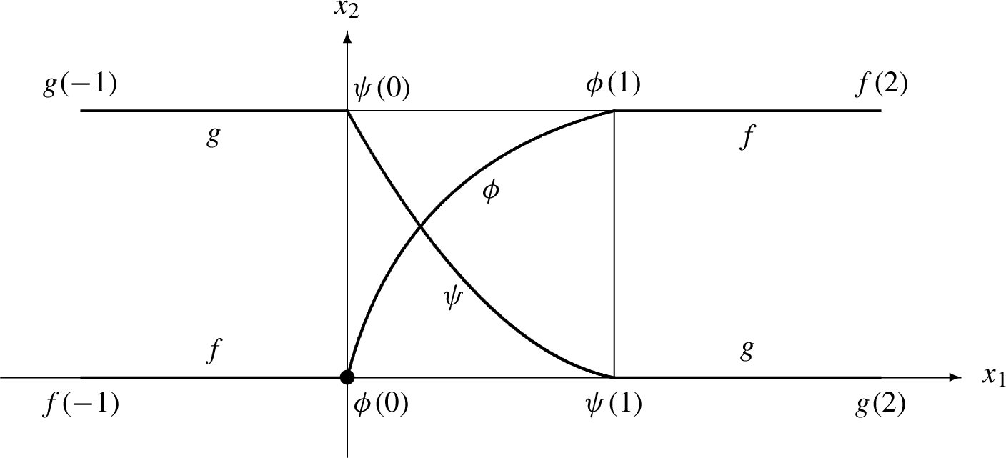
Figure 1 visualizes the theorem. In Markov-style computable analysis [4] Manukyan [7] has proved a related theorem (in Russian), cited in [5, Page 279] as follows: Theorem 1.2 (Manukyan).

There are two constructive (and therefore continuous) planar curves $φ_{1}$ and $φ_{2}$ such that $\begin{array}{l} (2) & φ_{1} (0) = (0, 0), φ_{1} (1) = (1, 1), φ_{2} (0) = (0, 1), φ_{1} (1) = (1, 0), \\ (3) & for every 0 < t < 1 both φ_{1} (t) and φ_{2} (t) belong to the open unit square, \\ (4) & the paths of φ_{1} and φ_{2} do not intersect. \end{array}$

While in (Grzegorczyk-Lacombe- [2,6]) computable analysis the following has been proved [10]:

Figure 1.

Intersecting curves ϕ and ψ with extensions f and g.

Theorem 1.3 (Weihrauch).

If ϕ and ψ in Theorem 1.1 are computable then there is a computable point $x \in range (ϕ) \cap range (ψ)$ .

This is not contradictory. In Markov’s approach only functions on the computable real numbers which are encoded by Gödel numbers are considered and computations transform Gödel numbers to Gödel numbers. While in the Grzegorczyk-Lacombe-approach all real numbers are considered, where real numbers are encoded by (fast converging) Cauchy sequences of rational numbers and computations transform infinite Cauchy sequences to infinite Cauchy sequences.

In this article we prove Claim 6.2 from [10]:

Theorem 1.4.
Let $T$ be the multi-valued operator mapping every pair $ϕ, ψ : [0; 1] \to {[0; 1]}^{2}$ of paths in the unit square such that $\begin{array}{l} (5) & ϕ (0) = (0, 0), ϕ (1) = (1, 1), ψ (0) = (0, 1) and ψ (1) = (1, 0) \end{array}$ to some pair $(S_{ϕ}, S_{ψ})$ of closed intervals such that $ϕ (S_{ϕ}) = ψ (S_{ψ})$ . Then the operator $T$ is computable.

Theorem 1.3 follows straightforwardly from Theorem 1.4. In the proof from ϕ and ψ we compute sequences $I_{0} \supseteq I_{1} \supseteq I_{2} \supseteq \dots$ and $J_{0} \supseteq J_{1} \supseteq J_{2} \supseteq \dots$ of closed intervals with rational endpoints such that $ϕ (⋂_{i} I_{i}) = ψ (⋂_{i} J_{i})$ .

Curves (even computable ones) can be much more complicated than the examples shown in Fig. 1. Consider, for example, space-filling curves or curves with infinitely many spirals, each of which containing infinitely many sub-spirals etc. infinitely often or curves with “completely” chaotic behavior.

This article is a contribution to computable analysis. There are various non equivalent definitions of computability in analysis. One of these is Markov’s constructive analysis [4,5]. Theorem 1.2 is a result in this theory. We use “TTE”, an approach which is based on ideas from [2,3,6]. In TTE computability on ${0, 1}^{}$ and Cantor space ${0, 1}^{ω}$ (the finite and infinite 0-1-sequences) is defined explicitly (e.g. by Turing machines with finite or infinite one-way input and output tapes) and computability on other sets X is induced via representations $δ : \subseteq {0, 1}^{} \to X$ or $δ : \subseteq {0, 1}^{ω} \to X$ (partial surjective) where finite or infinite 0-1-sequences are interpreted as names and computations are performed on names. We consider canonical representations of the real numbers, open subsets, closed subsets, compact subsets and real functions. Equivalently any finite alphabet Σ (with at least two elements) can be used instead of ${0, 1}$ . We assume that the reader is familiar with the basic concepts of TTE. Details can be found in [1,9,11].

For technical reasons we extend ϕ and ψ trivially to continuous functions $f, g : [- 1; 2] \to R^{2}$ which intersect in the same way as ϕ and ψ, that is, $ϕ (s) = ψ (t) ⟺ f (s) = g (t)$ (see Figure (1)): $\begin{array}{rcl} (6) & f (t) & : = & \{\begin{matrix} (t, 0) & if - 1 ⩽ t ⩽ 0 \\ ϕ (t) & if 0 ⩽ t ⩽ 1 \\ (t, 1) & if 1 ⩽ t ⩽ 2, \end{matrix} \\ (7) & g (t) & : = & \{\begin{matrix} (t, 1) & if - 1 ⩽ t ⩽ 0 \\ ψ (t) & if 0 ⩽ t ⩽ 1 \\ (t, 0) & if 1 ⩽ t ⩽ 2, \end{matrix} \end{array}$

We will consider closed rational sub-intervals $I = [a_{I}; b_{I}]$ and $J = [a_{J}; b_{J}]$ of the real interval $[- 1; 2]$ such that for the restrictions $f |_{I}$ of f to I and $g |_{J}$ of g to J, $\begin{array}{l} the end-points f |_{I} (a_{I}) and f |_{I} (b_{I}) are not in g (J) and \\ the end-points g |_{J} (a_{J}) and g |_{J} (b_{J}) are not in f (I) . \end{array}$ Since $f (I)$ and $g (J)$ are compact this means $\begin{array}{rcl} (8) & α_{I J} : = min (d_{s} ({f (a_{I}), f (b_{I})}, g (J)), d_{s} ({g (a_{J}), g (b_{J})}, f (I))) > 0, \end{array}$ where $d_{s} (A_{1}, A_{2}) : = inf {‖ z_{1} - z_{2} ‖ ∣ z_{1} \in A_{1}, z_{2} \in A_{2}}$ .

We will approximate $f |_{I}$ and $g |_{J}$ by rational polygon paths h and $h^{'}$ , respectively, and consider the intersections $(s, t)$ , that is, pairs such that $h (s) = h^{'} (t)$ . In order to keep this number finite we consider only pairs $(h, h^{'})$ such that $range (h) \cap range (h^{'})$ contains no straight line segment. For such pairs every intersection $(s, t)$ is either a crossing or tangent. As a central lemma we will prove that the parity (even or odd) of the number of crossings does not depend on h and $h^{'}$ (it is an invariant of $(f |_{I}, g |_{J})$ ). We call it the crossing parity of the pair $(f |_{I}, g |_{J})$ . In the proof we will apply transformations of polygon paths which may change the number of crossings but do not change the parity (even or odd) of the number of crossings.
2. The crossing parity

For points $x, y \in R^{2}$ such that $x \neq y$ let $\overline{x y} \subseteq R^{2}$ be the straight line segment from x to y. In this article $\overline{x x}$ is not a straight line segment.

Definition 2.1.

A track is a sequence $p = ((s_{0}, x_{0}), (s_{1}, x_{1}), \dots, (s_{k}, x_{k}))$ such that $s_{i} < s_{i + 1}$ and $x_{i} \neq x_{i + 1}$ for $0 ⩽ i < k$ . The points $x_{0}, x_{1}, \dots, x_{k}$ are the vertices of p.

The track p spans a (polygon) path $h_{p} : [s_{0}; s_{k}] \to R^{2}$ by $\begin{array}{l} (9) & h_{p} (s) & = x_{i} + \frac{s - s_{i}}{s_{i + 1} - s_{i}} (x_{i + 1} - x_{i}) if s_{i} ⩽ s ⩽ s_{i + 1} . \end{array}$

By Eq. (9), $h_{p} (s_{i}) = x_{i}$ and $h_{p} [s_{i}; s_{i + 1}] = \overline{x_{i} x_{i + 1}}$ .

For tracks p, q we want to count the number of crossings of the paths $h_{p}$ and $h_{q}$ . In order to keep this number finite we consider only pairs $(p, q)$ such that $range (h_{p})$ and $range (h_{q})$ have no common straight line segment. Furthermore, we will not count all intersections of $h_{p}$ and $h_{q}$ but only “proper” crossings.
Definition 2.2.
Let $(p, q)$ where $p = ((s_{0}, x_{0}), (s_{1}, x_{1}), \dots, (s_{k}, x_{k}))$ and $q = ((t_{0}, y_{0}), (t_{1}, y_{1}), \dots, (t_{l}, y_{l}))$ be a pair of tracks such that $range (h_{p})$ and $range (h_{q})$ have no common straight line segment.
An intersection of p and q is a pair $(s, t)$ such that $s_{0} < s < s_{k}$ , $t_{0} < t < t_{l}$ and $h_{p} (s) = h_{q} (t)$ . We call $x : = h_{p} (s) = h_{q} (t)$ the corresponding intersection point.

For an intersection $(s, t)$ of p and q with intersection point $h_{p} (s) = h_{q} (t) = x$ let $δ_{s t} > 0$ be a number such that $B (x, δ_{s t}) ∖ {x}$ contains no vertex of p and no vertex of q. Let $\begin{array}{l} s_{<} : = inf {s^{'} < s ∣ h_{p} [s^{'}; s] \subseteq B (x, δ_{s t})}, x_{<} : = h_{p} (s_{<}), \\ s_{>} : = sup {s^{'} > s ∣ h_{p} [s; s^{'}] \subseteq B (x, δ_{s t})}, x_{>} : = h_{p} (s_{>}), \\ t_{<} : = inf {t^{'} < t ∣ h_{q} [t^{'}; t] \subseteq B (x, δ_{s t})}, y_{<} : = h_{q} (t_{<}), \\ t_{>} : = sup {t^{'} > t ∣ h_{q} [t; t^{'}] \subseteq B (x, δ_{s t})}, y_{>} : = h_{q} (t_{>}) . 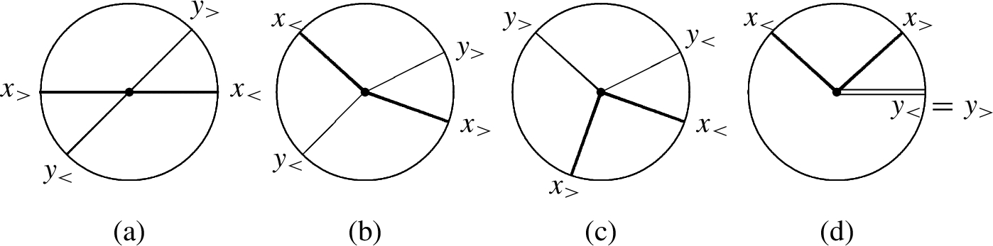\end{array}$ If on the boundary of $B (x, δ_{s t})$ the four points $x_{<}$ , $x_{>}$ , $y_{<}$ and $y_{>}$ occur in the order $(x_{<}, y_{<}, x_{>}, y_{>})$ or in the order $(x_{<}, y_{>}, x_{>}, y_{<})$ ,1
¹
That is, on the boundary of $B (x, δ_{s t})$ the four points alternate in x and y.

we call $(s, t)$ a crossing and x the corresponding crossing point, else x is a touch point.

Let $CN (p, q)$ be the number of crossings of p and q and let $π (p, q) : = CN (p, q) mod 2$ be its parity ( $0 =$ even and $1 =$ odd).

Obviously, $s_{<} < s_{i} < s$ for no number i, $x_{<} = h_{p} (s_{<}) \in \partial B (x, δ_{s t})$ and $h_{p} [s_{<}; s] = \overline{x_{<} x}$ where $\partial A$ denotes the boundary of $A \subseteq R^{2}$ . This is true correspondingly for $s_{>}$ , $t_{<}$ and $t_{>}$ .

Figure 2 shows several kinds of intersection of p and q (thin lines for $h_{q}$ and thick lines for $h_{p}$ ) the first two of which are crossings. In (a) possibly the center x is no vertex of p or no vertex of q.

Figure 2.
$h_{p}$ and $h_{q}$ in the ball $B (x, δ_{s t})$ for $x = h_{p} (s) = h_{q} (t)$ .

The definition of a crossing $(s, t)$ depends on the number $δ_{s t}$ only formally.
Lemma 2.3.
The definition of a crossing does not depend on the choice of $δ_{s t}$ .
Proof.
Let $(s, t)$ be a crossing of p and q defined via some $δ_{s t}$ . Let $0 < \overline{δ} < δ_{s t}$ .

Let ${\overline{s}}_{<} : = inf {s^{'} < s ∣ h_{p} [s^{'}; s] \subseteq B (x, \overline{δ})}$ and ${\overline{x}}_{<} : = h_{p} ({\overline{s}}_{<})$ . Then ${\overline{x}}_{<} = \overline{x_{<} x} \cap \partial B (x, \overline{δ})$ . This is true correspondingly for the other three cases. Obviously the four points on $\partial B (x, \overline{δ})$ alternate in the same way as the four corresponding points on $\partial B (x, δ_{s t})$ . □

Notice that ${x_{<}, x_{>}} \cap {y_{<}, y_{>}} = \emptyset$ since $range (h_{p})$ and $range (h_{q})$ have no common straight line segment. In the applications below the endpoints of $h_{p}$ are not in $range (h_{q})$ and the endpoints of $h_{q}$ are not in $range (h_{p})$ . Therefore it suffices to consider $s_{0} < s < s_{k}$ and $t_{0} < t < t_{l}$ in the definition of intersections.

We introduce a separation concept for tracks p and q which induces that $range (h_{p})$ and $range (h_{q})$ have no common straight line segment.
Definition 2.4.
Let $p = ((s_{0}, x_{0}), (s_{1}, x_{1}), \dots, (s_{k}, x_{k}))$ be a track.
Define $V (p) : = {x_{0}, x_{1}, \dots, x_{k}}$ .

For $x, y \in R^{2}$ with $x \neq y$ let $l (x, y)$ be the straight line through x and y.

Define $\begin{array}{l} (10) & L (p) : = ⋃ {l (x_{i - 1}, x_{i}) ∣ 1 ⩽ i ⩽ k}, \\ (11) & \overline{L} (p) : = ⋃ {l (x_{i}, x_{j}) ∣ 0 ⩽ i < j ⩽ k, x_{i} \neq x_{j}} . \end{array}$

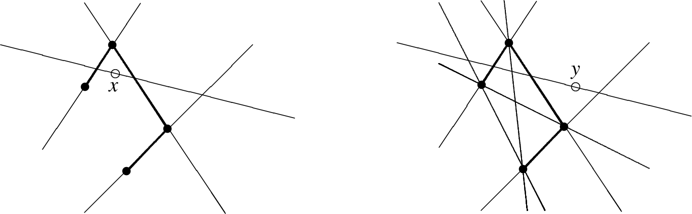
We call tracks p and q weakly separated, $p ⋈ q$ , iff $\begin{array}{l} (12) & V (p) \cap L (q) = \emptyset and \\ (13) & V (q) \cap L (p) = \emptyset . \end{array}$

Figure 3 shows on the left the set $L (p)$ of a track p and a straight line through a point $x \notin L (p)$ and on the right the set $\overline{L (q)}$ of a track q and a straight line through a point $y \notin \overline{L} (q)$ .

Figure 3.
$L (p)$ and $\overline{L} (q)$ .
Lemma 2.5.

If $y \notin L (p)$ then every straight line through the point y intersects every straight line from $L (p)$ at most once.

If $V (p) \cap L (q) = \emptyset$ or $V (q) \cap L (p) = \emptyset$ then then $range (h_{p})$ and $range (h_{q})$ have no common straight line segment.

Proof.
If a straight line through y intersects a straight line from $L (p)$ twice then $y \in L (p)$ . Contradiction.

Let $q = ((t_{0}, y_{0}), \dots, (t_{m}, y_{m}))$ . Suppose for some i and j, $\overline{x_{i} x_{i + 1}}$ and $\overline{y_{j} y_{j + 1}}$ have a common straight line segment. Then $x_{i} \in l (y_{j}, y_{j + 1}) \subseteq L (q)$ , but $V (p) \cap L (q) = \emptyset$ . Correspondingly, $V (q) \cap L (p) \neq \emptyset$ . □

As an essential tool we will use local transformations of tracks which leave the crossing parity invariant. The following lemma justifies these transformations.
Lemma 2.6.
Let $\begin{array}{l} p = ((s_{0}, x_{0}), (s_{1}, x_{1}), \dots, (s_{k}, x_{k})), \\ q_{1} = ((r, y), (t_{1}, z_{1}), (r^{'}, y^{'})) and \\ q_{2} = ((r, y), (t_{2}, z_{2}), (r^{'}, y^{'})) \end{array}$ be tracks and let B be a ball such that $\begin{array}{l} (14) & {y, y^{'}} \cap L (p) = \emptyset, \\ (15) & {y, y^{'}, z_{1}, z_{2}} \subseteq B, \\ (16) & {x_{0}, x_{k}} \cap B = \emptyset . \end{array}$ Then $π (p, q_{1}) = π (p, q_{2})$ .
Proof.
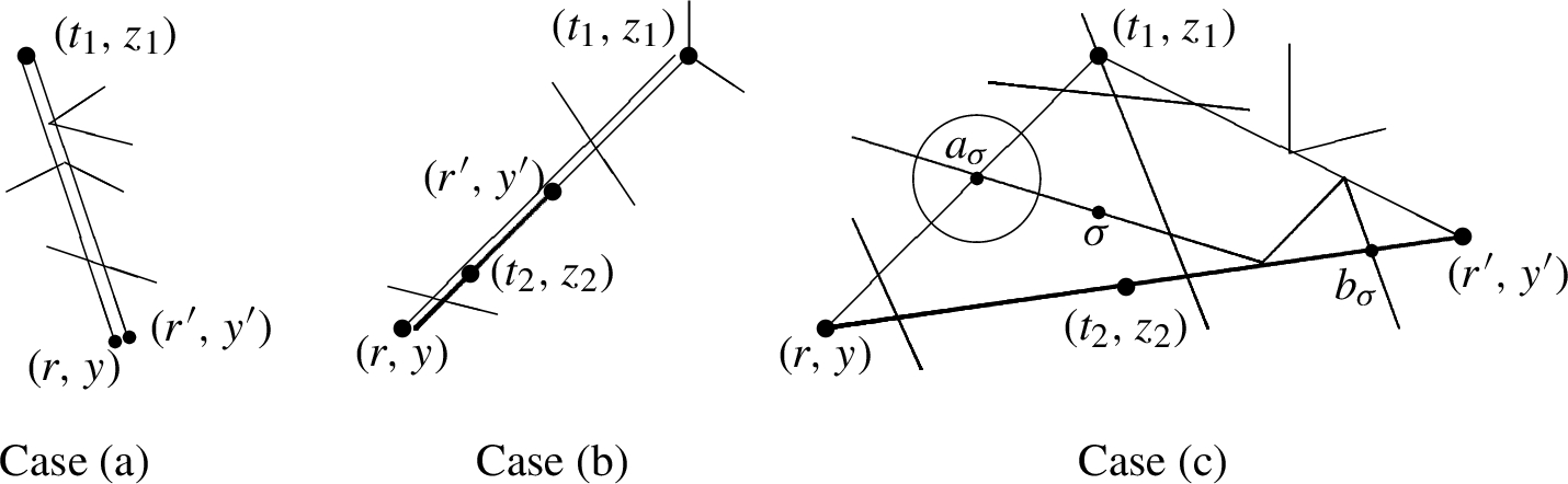
Remember that by Definition 2.1, $r < t_{1} < r^{'}$ , $r < t_{2} < r^{'}$ , $z_{1} \notin {y, y^{'}}$ and $z_{2} \notin {y, y^{'}}$ . By Eq. (14), $y, y^{'} \notin range (h_{p})$ .

If $range (h_{p})$ and $range (h_{q_{1}})$ have a common straight line segment then $y \in L (p)$ or $y^{'} \in L (p)$ , but ${y, y^{'}} \notin L (p)$ . Therefore, $CN (p, q_{1})$ is well-defined. Correspondingly, $CN (p, q_{2})$ is well-defined. We distinguish several cases, see Fig. 4. The “open ended” line segments are parts of $range (h_{p})$ .

Figure 4.
Illustration for Lemma 2.6.

Case (a) $y = y^{'}$ : Obviously, $CN (p, q_{1})$ and $CN (p, q_{2})$ are even, hence $π (p, q_{1}) = 0 = π (p, q_{2})$ .

Case (b) $y \neq y^{'}$ , $z_{2} \in \overline{y y^{'}}$ and $z_{1} \in l (y, y^{'})$ : In Fig. 4(b) the track $q_{2}$ is drawn in thick lines. If $z_{1} \in \overline{y y^{'}}$ then $CN (p, q_{1}) = CN (p, q_{2})$ . If $z_{1} \notin \overline{y y^{'}}$ then $CN (p, q_{1})$ and $CN (p, q_{2})$ differ by an even number. In both cases $π (p, q_{1}) = π (p, q_{2})$ .

Case (c) $y \neq y^{'}$ , $z_{2} \in \overline{y y^{'}}$ and $z_{1} \notin l (y, y^{'})$ : In Fig. 4(c) the track $q_{2}$ is drawn in thick lines. Let Δ be the closed triangle with boundary $\partial Δ : = range (h_{q_{1}}) \cup range (h_{q_{2}})$ ( $= \overline{y z_{1}} \cup \overline{z_{1} y^{'}} \cup \overline{y y^{'}}$ ) and let $Δ^{\circ}$ be its interior.

If $\overline{y z_{1}}$ and $range (h_{p})$ have a common straight line segment then $y \in L (p)$ , a contradiction by Eq. (14). Therefore $\overline{y z_{1}}$ and $range (h_{p})$ have no common straight line segment. This is true correspondingly for $\overline{z_{1} y^{'}}$ and $\overline{y y^{'}}$ . Therefore $\begin{array}{rcl} (17) & \partial Δ and range (h_{p}) have no common straight line segment. \end{array}$ Let $s_{0} < σ < s_{k}$ such that $h_{p} (σ) \in Δ^{\circ}$ . Let $[a_{σ}; b_{σ}]$ be the longest interval such that $s_{0} ⩽ a_{σ} < σ < b_{σ} ⩽ s_{k}$ and $h_{p} [a_{σ}; b_{σ}] \subseteq Δ$ . Figure 4(c) shows an example for σ with $a_{σ}$ and $b_{σ}$ positioned at the images under $h_{p}$ and $h_{p} (a_{σ}) \in range (h_{q_{1}})$ . Obviously, $h_{p} (a_{σ}), h_{p} (b_{σ}) \in Δ$ . We show that $h_{p} (a_{σ})$ and $h_{p} (b_{σ})$ are crossing points of p and $q_{1}$ or of p and $q_{2}$ .

Suppose $h_{p} (a_{σ}) \in range (h_{q_{1}})$

Since $range (h_{p})$ is a chain of straight line segments there is some $a_{σ} < s^{'} < σ$ such that $λ : = h_{p} ([a_{σ}; s^{'}])$ is a straight line segment with $h_{p} (a_{σ}) \in λ \cap \partial Δ$ and by Eq. (17) $λ ∖ {h_{p} (a_{σ})} \subseteq Δ^{\circ}$ .

Since $range (h_{p})$ is a chain of straight line segments and $a_{σ}$ is the smallest number a with $h_{p} [a; σ] \in Δ$ , there is some $s^{″} < a_{σ}$ such that $λ^{″} : = h_{p} [s^{″}; a_{σ}]$ is straight line segment with $h_{p} (a_{σ}) \in λ^{″} \cap \partial Δ$ and $(λ^{″} ∖ {h_{p} (a_{σ})}) \cap Δ = \emptyset$ by Eq. (17).

If we draw a sufficiently small circle around $h_{p} (a_{σ})$ then (with the terminology from Definition 2.2)) the intersections $x_{<}$ and $x_{>}$ of it with $range (h_{p})$ and the intersections $y_{<}$ and $y_{>}$ of it with $range (h_{q_{1}})$ alternate on this circle in x and y. Therefore, for every σ such that $h_{p} (σ) \in Δ^{\circ}$ , $\begin{matrix} h_{p} (a_{σ}) is a crossing point of p and q_{1} if h_{p} (a_{σ}) \in range (h_{q_{1}}) \end{matrix}$ and correspondingly, $\begin{array}{l} h_{p} (a_{σ}) is a crossing point of p and q_{2} if h_{p} (a_{σ}) \in range (h_{q_{2}}), \\ h_{p} (b_{σ}) is a crossing point of p and q_{1} if h_{p} (b_{σ}) \in range (h_{q_{1}}) and \\ h_{p} (b_{σ}) is a crossing point of p and q_{2} if h_{p} (b_{σ}) \in range (h_{q_{2}}) . \end{array}$ On the other hand, every crossing point of p and $q_{1}$ or $q_{2}$ is equal to $h_{p} (a_{σ})$ or $h_{p} (b_{σ})$ for some σ with $h_{p} (σ) \in Δ^{\circ}$ . Therefore, the number N of crossings of p with $q_{1}$ or $q_{2}$ is even. Since by Eq. (14) ${y, y^{'}} \cap range (h_{p}) = \emptyset$ , $N = CN (p, q_{1}) + CN (p, q_{2})$ is an even number, hence $π (p, q_{1}) = π (p, q_{2})$ .

Case (d) $y \neq y^{'}$ , $z_{2} \in l (y, y^{'}) ∖ \overline{y y^{'}}$ and $z_{1} \notin l (y, y^{'})$ : Let $q_{3} : = ((r, y), (t_{1}, z_{3}), (r^{'}, y^{'}))$ for $z_{3} : = (y_{1} + y_{2}) / 2$ . By Case (b), $π (p, q_{2}) = π (p, q_{3})$ and by Case (c), $π (p, q_{1}) = π (p, q_{3})$ .

Case (e) $y \neq y^{'}$ , $z_{1}, z_{2} \notin l (y, y^{'})$ : Let $q_{3} : = ((r, y), (t_{1}, z_{3}), (r^{'}, y^{'}))$ for $z_{3} : = (y_{1} + y_{2}) / 2$ . By Case (c), $π (p, q_{2}) = π (p, q_{3})$ and $π (p, q_{1}) = π (p, q_{3})$ .

Case (f) $y \neq y^{'}$ and $z_{1}, z_{2} \in l (y, y^{'}) ∖ \overline{y y^{'}}$ : Proof via $q_{3}$ as in (d) and (e). □

For tracks p, q and $q^{'}$ , by tiny shifts of the vertices of p we can obtain a track $\overline{p}$ such that $\overline{p} ⋈ q$ and $\overline{p} ⋈ q^{'}$ .
Lemma 2.7.

Let $p = ((s_{0}, x_{0}), (s_{1}, x_{1}) . \dots, (s_{k}, x_{k}))$ and let q and $q^{'}$ be tracks. Then for every $δ > 0$ there is some track $\overline{p} = ((s_{0}, y_{0}), (s_{1}, y_{1}), \dots, (s_{k}, y_{k}))$ such that $\overline{p} ⋈ q$ , $\overline{p} ⋈ q^{'}$ and $‖ x_{i} - y_{i} ‖ < δ$ for $0 ⩽ i ⩽ k$ .

If $p = ((s_{0}, x_{0}), (s_{1}, x_{1}) . \dots, (s_{k}, x_{k}))$ and $\overline{p} = ((s_{0}, y_{0}), (s_{1}, y_{1}), \dots, (s_{k}, y_{k}))$ are tracks such that $‖ x_{i} - y_{i} ‖ < δ$ for $0 ⩽ i ⩽ k$ then $‖ h_{p} (s) - h_{\overline{p}} (s) ‖ < δ$ for all $s_{0} ⩽ s ⩽ s_{k}$ .

Proof.

We must find (prove the existence of) points $y_{0}, y_{1}, \dots, y_{k}$ such that $‖ x_{i} - y_{i} ‖ < δ$ and for $\overline{p} : = ((s_{0}, y_{0}), (s_{1}, y_{1}), \dots, (s_{k}, y_{k}))$ , $\begin{array}{rcl} (18) & V (\overline{p}) \cap (L (q) \cup L (q^{'})) & = & \emptyset and \\ (19) & L (\overline{p}) \cap (V (q) \cup V (q^{'})) & = & \emptyset . \end{array}$ The following statements are true since $V (q) \cup V (q^{'})$ is a finite set of points and $L (q) \cup L (q^{'})$ is a finite set of straight lines.
There is some $y_{0} \in B (x_{0}, δ)$ such that $y_{0} \notin L (q) \cup L (q^{'})$ .

Suppose $y_{i}$ has been determined for some $0 ⩽ i < k$ . There is some $y_{i + 1} \in B (x_{i + 1}, δ)$ such that $\begin{matrix} y_{i + 1} \neq y_{i}, y_{i + 1} \notin (L (q) \cup L (q^{'})) and l (y_{i}, y_{i + 1}) \cap (V (q) \cup V (q^{'})) = \emptyset, \end{matrix}$
Then $\overline{p} : = ((s_{0}, y_{0}), (s_{1}, y_{1}) . \dots, (s_{k}, y_{k}))$ is a track such that $\overline{p} ⋈ q$ , $\overline{p} ⋈ q^{'}$ and $‖ x_{i} - y_{i} ‖ < δ$ for $0 ⩽ i ⩽ k$ .

For $s_{i} ⩽ s ⩽ s_{i + 1}$ by Eq. (9), $\begin{array}{rcl} ‖ h_{p} (s) - h_{\overline{p}} (s) ‖ & = & ‖ h_{p} (s_{i}) + \frac{s - s_{i}}{s_{i + 1} - s_{i}} (h_{p} (s_{i + 1}) - h_{p} (s_{i})) \\ - h_{\overline{p}} (s_{i}) - \frac{s - s_{i}}{s_{i + 1} - s_{i}} (h_{\overline{p}} (s_{i + 1}) - h_{\overline{p}} (s_{i})) ‖ \\ = & ‖ x_{i} + \frac{s - s_{i}}{s_{i + 1} - s_{i}} (x_{i + 1} - x_{i}) \\ - y_{i} - \frac{s - s_{i}}{s_{i + 1} - s_{i}} (y_{i + 1} - y_{i}) ‖ \\ = & ‖ (1 - \frac{s - s_{i}}{s_{i + 1} - s_{i}}) \cdot (x_{i} - y_{i}) \\ + \frac{s - s_{i}}{s_{i + 1} - s_{i}}) \cdot (x_{i + 1} - y_{i + 1}) ‖ \\ < & δ \end{array}$
□

In the following let $f, g : [- 1; 2] \to R^{2}$ , let $I = [a_{I}; b_{I}]$ and $J = [a_{J}; b_{J}]$ be intervals with rational endpoints such that $I, J \subseteq [- 1; 2]$ and let $α_{I J}$ be the number from Eq. ( 8 ).

Since f and g are continuous, there is a modulus of uniform continuity $md : N \to N$ for f and g, that is, $md$ is increasing and for all $t, t^{'} \in [- 1; 2]$ , $\begin{array}{rcl} (20) & ‖ f (t) - f (t^{'}) ‖ < 2^{- n} and ‖ g (t) - g (t^{'}) ‖ < 2^{- n} & if & | t - t^{'} | < 2^{- md (n)} . \end{array}$

We approximate $f |_{I}$ and $g |_{J}$ by tracks.
Definition 2.8.
A track $p = ((s_{0}, x_{0}), (s_{1}, x_{1}), \dots, (s_{k}, x_{k}))$ is an approximation with precision $2^{- n}$ (shortly an n-approximation) of $f |_{I}$ if $\begin{array}{l} (21) & s_{0} = a_{I} and s_{k} = b_{I}, \\ (22) & s_{i + 1} - s_{i} < 2^{- md (n)} and \\ (23) & ‖ f (s_{i}) - x_{i} ‖ < 2^{- n} . \end{array}$

Remember that by Definition 2.1, $x_{i} = h_{p} (s_{i})$ . Approximations of $g |_{J}$ are defined accordingly.
Lemma 2.9.
In Definition 2.8 , for all meaningful i and s, $\begin{array}{l} (24) & ‖ x_{i} - x_{i + 1} ‖ < 3 \cdot 2^{- n}, \\ (25) & ‖ f (s) - h_{p} (s) ‖ < 5 \cdot 2^{- n} . \end{array}$
Proof.
$‖ x_{i} - x_{i + 1} ‖ ⩽ ‖ x_{i} - f (s_{i}) ‖ + ‖ f (s_{i}) - f (s_{i + 1}) ‖ + ‖ f (s_{i + 1}) - x_{i + 1}) ‖ < 3 \cdot 2^{- n}$ .

For $s_{i} ⩽ s ⩽ s_{i + 1}$ , $‖ f (s) - h_{p} (s) ‖ ⩽ ‖ f (s) - f (s_{i}) ‖ + ‖ f (s_{i}) - h_{p} (s_{i}) ‖ + ‖ h_{p} (s_{i}) - h_{p} (s) ‖ < 2^{- n} + 2^{- n} + ‖ x_{i} - x_{i + 1} ‖ < 5 \cdot 2^{- n}$ by Eqs (9) and (24). □

After these technical preparations we prove the following central lemma.
Lemma 2.10.
Let $2^{- n} < α_{I J} / 16$ . Let p and $p^{'}$ be n-approximations of $f |_{I}$ and let q and $q^{'}$ be n-approximations of $g |_{J}$ such that $p ⋈ q$ and $p^{'} ⋈ q^{'}$ . Then $π (p, q) = π (p^{'}, q^{'})$ .
Proof.
Let $\begin{matrix} p = ((s_{0}, x_{0}), (s_{1}, x_{1}) . \dots, (s_{k}, x_{k})) \end{matrix}$ where $s_{0} = a_{I}$ and $s_{k} = b_{I}$ . Notice that possibly p and $q^{'}$ as well as $p^{'}$ and q have common straight line segments such that $π (p, q^{'})$ and $π (p^{'}, q)$ are not defined. By Lemma 2.7 there is some track $\begin{matrix} \overline{p} = ((s_{0}, y_{0}), (s_{1}, y_{1}), \dots, (s_{k}, y_{k})) \end{matrix}$ such that $\begin{array}{rcl} (26) & \overline{p} ⋈ q, & \overline{p} ⋈ q^{'} & and ‖ x_{i} - y_{i} ‖ < 2^{- n} for 0 ⩽ i ⩽ k . \end{array}$ Figure 5 shows the ⋈-relation (indicated by lines) between the tracks p, q, $\overline{p}$ , $p^{'}$ and $q^{'}$ . It suffices to prove $\begin{array}{rcl} (27) & π (p, q) = π (\overline{p}, q) = π (\overline{p}, q^{'}) = π (p^{'}, q^{'}) . \end{array}$ We use the facts that by the definitions the points $f (t)$ , $h_{p} (t)$ , $h_{\overline{p}} (t)$ and $h_{p^{'}} (t)$ are close together and that the points $g (t)$ , $h_{q} (t)$ and $h_{q^{'}} (t)$ are close together.
Figure 5.
The ⋈-relation between the tracks p, q, $\overline{p}$ , $p^{'}$ and $q^{'}$ .

In the following we prove the second equation $π (\overline{p}, q) = π (\overline{p}, q^{'})$ of Eq. (27) in detail. Let $\begin{array}{l} (28) & q = ((r_{0}, u_{0}), (r_{1}, u_{1}), \dots, (r_{l - 1}, u_{l - 1}), (r_{l}, u_{l})), \\ (29) & q^{'} = ((r_{0}^{'}, u_{0}^{'}), (r_{1}^{'}, u_{1}^{'}), \dots, (r_{m - 1}^{'}, u_{m - 1}^{'}), (r_{m}^{'}, u_{m}^{'})) \\ (30) & where r_{0} = r_{0}^{'} = a_{J} and r_{l} = r_{m}^{'} = b_{J} . \end{array}$ be n-approximations of $g |_{J}$ . As an example, Fig. 6 shows the arguments $r_{0}, \dots, r_{6}$ of a track q on the real line and and the arguments $r_{0}^{'}, \dots, r_{7}^{'}$ of a track $q^{'}$ on the real line (thick black dots).

Figure 6.
Insertion of redundant vertices into q and $q^{'}$ .

From Eq. (26) we know that $V (q) \cap L (\overline{p}) = \emptyset$ and $V (q^{'}) \cap L (\overline{p}) = \emptyset$ . In a first step we add “redundant” vertices to q and $q^{'}$ such that the resulting tracks $q_{1}$ and $q_{1}^{'}$ have the same number of vertices and such that $h_{q} = h_{q_{1}}$ , $h_{q^{'}} = h_{q_{1}^{'}}$ , $V (q_{1}) \cap L (\overline{p}) = \emptyset$ and $V (q_{1}^{'}) \cap L (\overline{p}) = \emptyset$ .

Let i be a number such that $r_{i} \notin {r_{0}^{'}, \dots, r_{m}^{'}}$ . There is a unique j such that $r_{j}^{'} < r_{i} < r_{j + 1}^{'}$ (e.g. $i = 3$ and $j = 1$ in Fig. 6).

The point $h_{q^{'}} (r_{i})$ is an element of the straight line segment $\overline{u_{j}^{'} u_{j + 1}^{'}}$ and different from $u_{j}^{'}$ and $u_{j + 1}^{'}$ . We would like to add the “redundant” pair $(r_{i}, h_{q^{'}} (r_{i}))$ to $q^{'}$ with result $\begin{matrix} ((r_{0}^{'}, u_{0}^{'}), \dots, (r_{j}^{'}, u_{j}^{'}), (r_{i}, h_{q^{'}} (r_{i})), (r_{j + 1}^{'}, u_{j + 1}^{'}), \dots, (r_{m}^{'}, u_{m}^{'})) \end{matrix}$ But possibly $h_{q^{'}} (r_{i}) \in L (\overline{p})$ . Instead, we add a pair $(t, v)$ with $v = h_{q^{'}} (t) \notin L (\overline{p})$ to $q^{'}$ which is very close to $(r_{i}, h_{q^{'}} (r_{i}))$ . Let $\begin{array}{rcl} (31) & γ : = min {| c - d | ∣ c, d \in {r_{0}, \dots, r_{l}, r_{0}^{'}, \dots, r_{m}^{'}} and c \neq d} . \end{array}$ Since $u_{j}^{'} \notin L (\overline{p})$ , by Lemma 2.5 $l (u_{j}^{'} u_{j + 1}^{'})$ intersects every straight line from $L (\overline{p})$ at most once. Therefore, the straight line segment $\overline{u_{j}^{'} u_{j + 1}^{'}}$ contains only finitely many points of $L (\overline{p})$ . Thus there is some t such that $| t - r_{i} | < γ / 8$ and $v : = h_{q^{'}} (t) \notin L (\overline{p})$ . Then $v \in \overline{u_{j}^{'} u_{j + 1}^{'}}$ (see Eq. (9)). We add the pair $(t, v)$ to $q^{'}$ with result $\begin{matrix} \overline{q} : = ((r_{0}^{'}, u_{0}^{'}), \dots, (r_{j}^{'}, u_{j}^{'}), (t, h_{q^{'}} (t)), (r_{j + 1}^{'}, u_{j + 1}^{'}), \dots, (r_{m}^{'}, u_{m}^{'})) . \end{matrix}$ Then $h_{q^{'}} = h_{\overline{q}}$ . Let $q_{1}^{'}$ be the track obtained from $q^{'}$ by adding a pair $(t, v)$ in this way for every i such that $r_{i} \notin {r_{0}^{'}, \dots, r_{m}^{'}}$ in turn. Then $h_{q^{'}} = h_{q_{1}^{'}}$ and $V (q_{1}^{'}) \cap L (\overline{p}) = \emptyset$ .

Correspondingly let $q_{1}$ be the track obtained from q in the same way. Then $h_{q} = h_{q_{1}}$ and $V (q_{1}) \cap L (\overline{p}) = \emptyset$ . In summary, $\begin{array}{rcl} (32) & h_{q} = h_{q_{1}}, h_{q^{'}} = h_{q_{1}^{'}}, V (q_{1}) \cap L (\overline{p}) = \emptyset and V (q_{1}^{'}) \cap L (\overline{p}) = \emptyset . \end{array}$

In Fig. 6 the inserted arguments t are within the circles. The new tracks can be written as $\begin{array}{rcl} (33) & q_{1} & = & ((t_{0}, v_{0}), (t_{1}, v_{1}), \dots, (t_{μ}, v_{μ})), \\ (34) & q_{1}^{'} & = & ((t_{0}^{'}, v_{0}^{'}), (t_{1}^{'}, v_{1}^{'}), \dots, (t_{μ}^{'}, v_{μ}^{'})) \end{array}$ where $a_{J} = r_{0} = t_{0} = t_{0}^{'}$ and $b_{J} = r_{l} = t_{μ} = t_{μ}^{'}$ . By the condition $| t - r_{i} | < γ / 8$ in the definition of $(t, v)$ above, $\begin{array}{l} (35) & | t_{ν} - t_{ν}^{'} | < γ / 8 and {t_{ν}, t_{ν}^{'}} < {t_{ν + 1}, t_{ν + 1}^{'}} . \end{array}$ The next Proposition prepares the proof of Proposition 2.12. Proposition 2.11.
For the tracks $q_{1}$ and $q_{1}^{'}$ , for all $0 < ν < μ$ , $\begin{array}{l} (36) & {v_{ν - 1}, v_{ν}, v_{ν + 1}, v_{ν - 1}^{'}, v_{ν}^{'}, v_{ν + 1}^{'}} \subseteq B (g (t_{ν}), 9 \cdot 2^{- n}) and \\ (37) & {y_{0}, y_{k}} \cap B (g (t_{ν}), 14 \cdot 2^{- n}) = \emptyset, \\ (38) & B (g (t_{1}), 9 \cdot 2^{- n}) \cap range (h_{\overline{p}}) = \emptyset, \\ (39) & B (g (t_{μ - 1}), 9 \cdot 2^{- n}) \cap range (h_{\overline{p}}) = \emptyset . \end{array}$
Proof of Proposition 2.11.
Proof of Eq. ( 36 ): Consider $((t_{ν - 1}, v_{ν - 1}), (t_{ν}, v_{ν}), (t_{ν + 1}, v_{ν + 1}))$ as a part of $q_{1}$ . Then $(t_{ν}, v_{ν})$ has already been in q, that is, $(t_{ν}, v_{ν}) = (r_{i}, u_{i})$ for some i or it has been inserted via some j such that $r_{j}^{'} \notin {r_{0}, \dots, r_{l}}$ . Therefore, there is some i such that (see Fig. 6) $\begin{array}{l} (40) & r_{i - 1} ⩽ t_{ν - 1} < r_{i} < t_{ν + 1} ⩽ r_{i + 1} or \\ (41) & r_{i} ⩽ t_{ν - 1} < t_{ν} < t_{ν + 1} ⩽ r_{i + 1} . \end{array}$

Consider Eq. (40). Then $‖ g (t_{ν}) - v_{ν} ‖ = ‖ g (r_{i}) - u_{i} ‖ < 2^{- n}$ by Eq. (23). Furthermore, $‖ g (t_{ν}) - v_{ν - 1} ‖ ⩽ ‖ g (t_{ν}) - v_{ν} ‖ + ‖ v_{ν} - v_{ν - 1} ‖ < 2^{- n} + ‖ u_{i} - v_{ν - 1} ‖$ . Since $h_{q} = h_{q_{1}}$ , $v_{ν - 1} \in \overline{u_{i - 1} u_{i}}$ , hence $‖ u_{i} - v_{ν - 1} ‖ ⩽ ‖ u_{i - 1} - u_{i} ‖ < 3 \cdot 2^{- n}$ by Eq. (24). Therefore, $‖ g (t_{ν}) - v_{ν - 1} ‖ < 4 \cdot 2^{- n}$ . By symmetry $‖ g (t_{ν}) - v_{ν + 1} ‖ < 4 \cdot 2^{- n}$ . Therefore, ${v_{ν - 1}, v_{ν}, v_{ν + 1}} \subseteq B (g (t_{ν}), 4 \cdot 2^{- n})$ .

Consider Eq. (41).Then

$‖ g (t_{ν}) - v_{ν} ‖ = ‖ g (t_{ν}) - h_{q} (t_{ν}) ‖ < 5 \cdot 2^{- n}$ by Eq. (25). Furthermore, $‖ g (t_{ν}) - v_{ν - 1} ‖ ⩽ ‖ g (t_{ν}) - v_{ν} ‖ + ‖ v_{ν} - v_{ν - 1} ‖ < 5 \cdot 2^{- n} + ‖ u_{i + 1} - u_{i} ‖ < 5 \cdot 2^{- n} + 3 \cdot 2^{- n} = 8 \cdot 2^{- n}$ (since $v_{ν}, v_{ν - 1} \in \overline{u_{i} u_{i + 1}}$ and by Eq. (24)). By symmetry $‖ g (t_{ν}) - v_{ν + 1} ‖ < 8 \cdot 2^{- n}$ . Therefore, ${v_{ν - 1}, v_{ν}, v_{ν + 1}} \subseteq B (g (t_{ν}), 8 \cdot 2^{- n})$ .

As a summary, in both cases Eqs (40) and (41), ${v_{ν - 1}, v_{ν}, v_{ν + 1}} \subseteq B (g (t_{ν}), 8 \cdot 2^{- n})$ . By symmetry, ${v_{ν - 1}^{'}, v_{ν}^{'}, v_{ν + 1}^{'}} \subseteq B (g (t_{ν}^{'}), 8 \cdot 2^{- n})$ . Since $| t_{ν} - t_{ν}^{'} | < γ / 4 < 2^{- md (n)}$ , $‖ g (t_{ν}) - g (t_{ν}^{'} ‖ < 2^{- n}$ by Eqs (35), (31), (22) and (20). Therefore, ${v_{ν - 1}, v_{ν}, v_{ν + 1}, v_{ν - 1}^{'}, v_{ν}^{'}, v_{ν + 1}^{'}} \subseteq B (g (t_{ν}), 9 \cdot 2^{- n})$ .

Proof of Eq. ( 37 ): By Eqs (8), (23) and Lemma 2.7 for all ν

$16 \cdot 2^{- n} < α_{I J} ⩽ ‖ f (s_{0}) - g (t_{ν}) ‖ ⩽ ‖ f (s_{0}) - x_{0} ‖ + ‖ x_{0} - y_{0} ‖ + ‖ y_{0} - g (t_{ν}) ‖ < 2^{- n} + 2^{- n} + ‖ y_{0} - g (t_{ν}) ‖$ , hence $‖ y_{0} - g (t_{ν}) ‖ > 14 \cdot 2^{- n}$ . By symmetry, $‖ y_{k} - g (t_{ν}) ‖ > 14 \cdot 2^{- n}$ .

Proof of Eq. ( 38 ): For every $s_{0} ⩽ s ⩽ s_{k}$ , $‖ f (s) - g (r_{0}) ‖ ⩾ α_{I J} > 16 \cdot 2^{- n}$ . By Eq. (25) and Lemma 2.7, $‖ h_{\overline{p}} (s) - g (r_{0}) ‖ > 10 \cdot 2^{- n}$ . Since $| r_{0} - t_{1} | ⩽ | r_{0} - r_{1} | < 2^{md} (n)$ , $‖ h_{\overline{p}} (s) - g (t_{1}) ‖ > 9 \cdot 2^{- n}$ , hence $B (g (t_{1}), 9 \cdot 2^{- n}) \cap range (h_{\overline{p}}) = \emptyset$ .

Proof of Eq. ( 39 ): From Eq. (38) by symmetry. □
Proposition 2.12.
$π (\overline{p}, q_{1}) = π (\overline{p}, q_{1}^{'})$ .
Proof of Proposition 2.12.
We transform the track $q_{1}^{'}$ in two phases to the track $q_{1}$ preserving the crossing parity in each step. Remember Eq. (32) and Proposition 2.11 for $\begin{array}{rcl} q_{1} & = & ((t_{0}, v_{0}), (t_{1}, v_{1}), (t_{2}, v_{2}), \dots, (t_{μ}, v_{μ})) and \\ q_{1}^{'} & = & ((t_{0}^{'}, v_{0}^{'}), (t_{1}^{'}, v_{1}^{'}), (t_{2}^{'}, v_{2}^{'}), \dots, (t_{μ}^{'}, v_{μ}^{'})) . \end{array}$

In the first phase for every $0 ⩽ i < μ$ we replace every $v_{i}^{'}$ by some $w_{i}$ without changing $q_{i}^{'}$ . For $0 ⩽ i < μ$ let $Q (i)$ be the following property:

There are points $w_{0}, \dots, w_{i}$ such that for all $1 ⩽ j ⩽ i$ $\begin{array}{l} (42) & ‖ w_{j} - v_{j}^{'} ‖ < 2^{- n} / 16, w_{j} \notin L (\overline{p}), w_{j} \notin {v_{j - 1}, w_{j - 1}, v_{j + 1}^{'}}) and \\ (43) & π (\overline{p}, q_{1}^{'}) = π (\overline{p}, {\overline{q}}_{i}) \end{array}$ where ${\overline{q}}_{i}$ is the track $\begin{matrix} {\overline{q}}_{i} : = ((t_{0}^{'}, w_{0}), \dots, (t_{i}^{'}, w_{i}), (t_{i + 1}^{'}, v_{i + 1}^{'}), \dots, (t_{μ}^{'}, v_{μ}^{'})) . \end{matrix}$

Let $w_{0} : = v_{0}^{'}$ . Then $q_{1}^{'} = {\overline{q}}_{0}$ , hence $Q (0)$ is true. Suppose for some $0 ⩽ i ⩽ μ - 2$ we have proved $Q (i)$ . There is some $w_{i + 1}$ such that $\begin{array}{rcl} (44) & ‖ w_{i + 1} - v_{i + 1}^{'} ‖ < 2^{- n} / 16, w_{i + 1} \notin L (\overline{p}), w_{i + 1} \notin {v_{i}, w_{i}, v_{i + 2}^{'}} . \end{array}$ By definition, $\begin{array}{l} {\overline{q}}_{i} = ((t_{0}^{'}, w_{0}), \dots, (t_{i}^{'}, w_{i}), (t_{i + 1}^{'}, v_{i + 1}^{'}), (t_{i + 2}^{'}, v_{i + 2}^{'}), \dots, (t_{μ}^{'}, v_{μ}^{'})) and \\ {\overline{q}}_{i + 1} = ((t_{0}^{'}, w_{0}), \dots, (t_{i}^{'}, w_{i}), (t_{i + 1}^{'}, w_{i + 1}), (t_{i + 2}^{'}, v_{i + 2}^{'}), \dots, (t_{μ}^{'}, v_{μ}^{'})) . \end{array}$ Since ${\overline{q}}_{i}$ is a track, by Eq. (44), ${\overline{q}}_{i + 1}$ is a track (neighboring vertices must be different). Also by Eq. (44), Eq. (42) is true also for $i + 1$ . By Proposition 2.11 Lemma 2.6 can be applied to the boldface sub-tracks $τ_{1} : = ((t_{i}^{'}, w_{i}), (t_{i + 1}^{'}, v_{i + 1}^{'}), (t_{i + 2}^{'}, v_{i + 2}^{'}))$ and $τ_{2} : = ((t_{i}^{'}, w_{i}), (t_{i + 1}^{'}, w_{i + 1}), (t_{i + 2}^{'}, v_{i + 2}^{'}))$ such that $π (\overline{p}, τ_{1}) = π (\overline{p}, τ_{2})$ . Since the vertices of ${\overline{q}}_{i}$ and ${\overline{q}}_{i + 1}$ are not in $L (\overline{p})$ , hence not in $range (h_{\overline{p}})$ , $π (\overline{p}, q_{1}^{'}) = π (\overline{p}, {\overline{q}}_{i}) = π (\overline{p}, {\overline{q}}_{i + 1})$ . Therefore, we have proved $Q (i + 1)$ .

By induction $Q (μ - 1)$ is true, hence $\begin{array}{rcl} (45) & π (\overline{p}, q_{1}^{'}) = π (\overline{p}, {\overline{q}}_{μ - 1}) . \end{array}$

Figure 7 shows the ≠-relation for the vertices of
$q_{1} = ((t_{0}, v_{0}), (t_{1}, v_{1}), (t_{2}, v_{2}), \dots, (t_{μ}, v_{μ}))$ (top) and

${\overline{q}}_{μ - 1} = ((t_{0}^{'}, w_{0}), (t_{1}^{'}, w_{1}), \dots, (t_{μ - 1}^{'}, w_{μ - 1}), (t_{μ}^{'}, v_{μ}^{'}))$ (bottom). A line between x and y means $x \neq y$ .

Figure 7.
The ≠-relation for the vertices of $q_{1}$ (top) and ${\overline{q}}_{μ - 1}$ (bottom).

In the second phase two we transform ${\overline{q}}_{μ - 1}$ step by step to $q_{1}$ without changing the crossing parity with $\overline{p}$ . For $0 ⩽ i ⩽ μ - 1$ let $\begin{matrix} q_{i}^{″} : = ((t_{0}, v_{0}), \dots, (t_{i}, v_{i}), (t_{i + 1}^{'}, w_{i + 1}), \dots, (t_{μ - 1}^{'}, w_{μ - 1}), (t_{μ}^{'}, v_{μ}^{'})) . \end{matrix}$ Since $q_{1}$ and ${\overline{q}}_{μ - 1}$ are tracks and $v_{i} \neq w_{i + 1}$ , $q_{i}^{″}$ is a track.

By Eq. (36) and by $‖ w_{1} - v_{1}^{'} ‖ < 2^{- n} / 16$ (Eq. (42)), $\overline{v_{0} w_{1}} \cup \overline{w_{0} w_{1}} \subseteq B (g (t_{1}), 6 \cdot 2^{- n})$ . By Eq. (38), $\overline{v_{0} w_{1}}$ and $\overline{w_{0} w_{1}}$ do not intersect $h_{\overline{p}}$ . Therefore, $\begin{array}{rcl} (46) & π (\overline{p}, {\overline{q}}_{μ - 1}) & = & π (\overline{p}, q_{0}^{″}) \end{array}$

Suppose for $0 ⩽ i ⩽ μ - 3$ $\begin{matrix} π (\overline{p}, {\overline{q}}_{μ - 1}) = π (\overline{p}, q_{i}^{″}) . \end{matrix}$ By definition, $\begin{array}{l} q_{i}^{″} = ((t_{0}, v_{0}), \dots, (t_{i}, v_{i}), (t_{i + 1}^{'}, w_{i + 1}), (t_{i + 1}^{'}, w_{i + 2}), \dots, (t_{μ}^{'}, v_{μ}^{'})) and \\ q_{i + 1}^{″} = ((t_{0}, v_{0}), \dots, (t_{i}, v_{i}), (t_{i + 1}, v_{i + 1}), (t_{i + 1}^{'}, w_{i + 2}), \dots, (t_{μ}^{'}, v_{μ}^{'})), \end{array}$

By Proposition 2.11 Lemma 2.6 can be applied to the boldface sub-tracks $\begin{array}{l} τ_{1} : = ((t_{i}, v_{i}), (t_{i + 1}^{'}, w_{i + 1}), (t_{i + 1}^{'}, w_{i + 2}) and \\ τ_{2} : = ((t_{i}, v_{i}) (t_{i + 1}, v_{i + 1}), (t_{i + 1}^{'}, w_{i + 2})) \end{array}$ such that $π (\overline{p}, τ_{1}) = π (\overline{p}, τ_{2})$ .

Since the vertices of ${\overline{q}}_{i}^{″}$ and ${\overline{q}}_{i + 1}^{″}$ are not in $L (\overline{p})$ , hence not in $range (h_{\overline{p}})$ , $π (\overline{p}, {\overline{q}}_{μ - 1}) = π (\overline{p}, q_{i}^{″}) = π (\overline{p}, q_{i + 1}^{″})$ . By induction, $\begin{matrix} π (\overline{p}, {\overline{q}}_{μ - 1}) = π (\overline{p}, q_{μ - 2}^{″}) \end{matrix}$ Finally we compare $\begin{array}{l} q_{1} = ((t_{0}, v_{0}), \dots, (t_{μ - 2}, v_{μ - 2}), (t_{μ - 1}, v_{μ - 1}), (t_{μ}, v_{μ})) and \\ q_{μ - 2}^{″} = ((t_{0}, v_{0}), \dots, (t_{μ - 2}, v_{μ - 2}), (t_{μ - 1}^{'}, w_{μ - 1}), (t_{μ}^{'}, v_{μ}^{'})) . \end{array}$

Since $‖ w_{μ - 1} - v_{μ - 1}^{'} ‖ < 2^{- n}$ by Proposition 2.11 and $\begin{matrix} (\overline{v_{μ - 2} v_{μ - 1}} \cup \overline{v_{μ - 1} v_{μ}} \cup \overline{v_{μ - 2} w_{μ - 1}} \cup \overline{w_{μ - 1} v_{μ}^{'}}) \cap range (h_{\overline{p}}) = \emptyset, \end{matrix}$

$π (\overline{p}, q_{μ - 2}^{″}) = π (\overline{p}, q_{1})$ , hence $π (\overline{p}, q_{1}^{'}) = π (\overline{p}, q_{1})$ . □

We continue the proof of Lemma 2.10. Since $h_{q} = h_{q_{1}}$ and $h_{q^{'}} = h_{q_{1}^{'}}$ by Eq. (32), $π (\overline{p}, q^{'}) = π (\overline{p}, q)$ , which is the second equation from Eq. (27). The first and the third equation can be poved accordingly. We omit the details. □

Lemma 2.10 allows to define the parity of the pair $(f |_{I}, g |_{J})$ .
Definition 2.13.
$π (f |_{I}, g |_{J}) : = π (p, q)$ for an arbitrary n-approximation p of $f |_{I}$ and an arbitrary n-approximation q of $g |_{J}$ such that $p ⋈ q$ and $2^{- n} < α_{I J} / 16$ .
Lemma 2.14.
Let f, g, J and $I = [a_{I}; b_{I}]$ be as before such that Eq. ( 8 ). Let $I_{1} : = [a_{I}; c]$ and $I_{2} : = [c; b_{I}]$ where $a_{I} < c < b_{I}$ and $f (c) \notin g (J)$ . Then $\begin{array}{rcl} (47) & π (f |_{I}, g |_{J}) = (π (f |_{I_{1}}, g |_{J}) + π (f |_{I_{2}}, g |_{J})) mod 2 . \end{array}$
Proof.
There are numbers $α > 0$ and $n \in N$ such that

$α < d_{s} ({f (a_{I}), f (c), f (b_{I})}, g (J))$ , $α < d_{s} ({g (a_{J}), g (b_{J})}, f (I))$ and $16 \cdot 2^{- n} < α$ . There are n-approximations $p = ((s_{0}, x_{0}), \dots, (s_{k}, x_{x}))$ and q of $f |_{I}$ and $g |_{J}$ , respectively, such that $c = s_{i}$ for some i and $p ⋈ q$ .

Let $p_{1} : = ((s_{0}, x_{0}), \dots, (s_{i}, x_{i}))$ and $p_{2} : = ((s_{i}, x_{i}), \dots, (s_{k}, x_{k}))$ .

Then $p_{1} ⋈ q$ and $p_{2} ⋈ q$ . Therefore $CN (p_{1}, q)$ and $CN (p_{2}, q)$ are well-defined such that (see Definition 2.2) $\begin{matrix} CN (p, q) = CN (p_{1}, q) + CN (p_{2}, q), \end{matrix}$ hence $π (p, q) = CN (p, q) mod 2 = (CN (p_{1}, q) mod 2 + CN (p_{2}, q) mod 2) mod 2 = (π (p_{1}, q) + π (p_{2}, q)) mod 2$ . Equation (47) follows by Definition 2.13. □
3. Crossing parities can be computed

In TTE computability is defined on represented sets $(X, δ)$ . A representation is a function $δ : \subseteq Σ^{*} \to X$ (if X is finite) or $δ : \subseteq Σ^{ω} \to X$ (if X has at most continuum cardinality). If $δ (w) = x$ then w is considered as a “name” (or a “δ-name”) of x. Every $x \in X$ must have a name (and may have many names) but not every $w \in Σ^{*}$ must be a name of some $x \in X$ , hence δ is a partial surjective function.

For represented sets $(X_{i}, δ_{i})$ where $δ_{i} : \subseteq A_{i} \to X_{i}$ , $A_{i} \in {Σ^{*}, Σ^{ω}}$ , a partial function $f : \subseteq X_{1} \to X_{2}$ is computable, if there is a computable function $h : \subseteq A_{1} \to A_{2}$ which realizes f, that is, if w is a $δ_{1}$ -name of $x \in dom (f)$ then $h (w)$ is a $δ_{2}$ -name of $f (x)$ (accordingly functions on Cartesian products). For most sets in Analysis there are canonical (or standard or effective or obvious) representations which we use here. We will say “computable” without mentioning the (standard) representations.

We need the concept of computable multi-functions on represented sets. As an example, for the standard represented sets $(R, ρ)$ , $(Q, ν_{Q})$ and $(N, ν_{N})$ there is no computable function $f : R \times N \to Q$ such that $| x - f (x, n) | < 2^{- n}$ . But there is a computable function $h : Σ^{ω} \times Σ^{*} \to Σ^{*}$ which from every name of x and every name of n computes a name of some $a \in Q$ such that $| x - a | < 2^{- n}$ . The computed number a depends on the names of x and n and not only on $(x, n)$ . The function h realizes the multi-function $f : R \times N ⇉ Q$ such that $f (x, n) = {a \in Q ∣ | x - a | < 2^{- n}}$ . Informally we say: f maps every $(x, n)$ to some $a \in Q$ such that $| x - a | < 2^{- n}$ , more formally, such that $| x - a | < 2^{- n}$ . In the following we apply results about computability on sets with standard representations from [1 ,8 ,9 ,11].

In Lemma 3.1 we consider n-approximations p and q of $f |_{I}$ and $g |_{J}$ , respectively such that $p ⋈ q$ . We prove that p and q can be computed from $(f, g, I, J, n)$ . We use from TTE, that ( $s \in Q, y \in Q^{2}$ ) such that $‖ f (s) - y ‖ < 2^{- n}$ ) is computable.

Lemma 3.1.
Let be the multi-function mapping continuous functions $f, g : [- 1; 2] \to R^{2}$ , closed rational intervals $I, J \subseteq [- 1; 2]$ and a number $n \in N$ to a pair $(p, q)$ , $p = ((s_{0}, x_{0}), \dots, (s_{k}, x_{k}))$ and $q = ((t_{0}, y_{0}), \dots, (t_{l}, y_{l}))$ , of rational tracks such that $\begin{array}{l} (48) & p is an n -approximation of f |_{I}, \\ (49) & q is an n -approximation of g |_{J} and \\ (50) & p ⋈ q . \end{array}$ Then $R$ is computable.

Since rational tracks are “discrete” objects there is no compuble funtion but only a computable multi-function (known from TTE).
Proof.
It is known [1 ,9,11] that from continuous functions $f, g : [- 1; 2] \to R^{2}$ we can compute a modulus of continuity ${md}_{f}$ of f and a modulus of continuity ${md}_{g}$ of g. We can compute $md : = max ({md}_{f}, {md}_{g})$ , which is a modulus of continuity of f and of g. Let $I = [a_{I}; b_{I}]$ and $J = [a_{J}; b_{J}]$ . Consider Definition 2.8.

First we compute p.

Choose some k and rational numbers $s_{0} : = a_{I}, s_{1}, \dots, s_{k - 1}, s_{k} : = b_{I}$ such that $0 < s_{i + 1} - s_{i} < 2^{- md (n)}$ for $0 ⩽ i < k$ . Choose some $x_{0} \in Q^{2}$ such that $‖ f (s_{0}) - x_{0} ‖ < 2^{- n}$ . Suppose, $x_{i}$ has been chosen for $i < k$ . Then choose some $x_{i + 1} \in Q^{2}$ such that $‖ f (s_{i + 1}) - x_{i + 1} ‖ < 2^{- n}$ and $x_{i + 1} \neq x_{i}$ . Since $x_{i} \neq x_{i + 1}$ for $i < k$ , $p : = ((s_{0}, x_{0}), \dots, (s_{k}, x_{k}))$ is a rational track. It is an n-approximation of $f |_{I}$ .

Next we compute q.

Choose some l and rational numbers $t_{0} : = a_{J}, t_{1}, \dots, t_{l - 1}, t_{l} : = b_{J}$ such that $0 < t_{i + 1} - t_{i} < 2^{- md (n)}$ for $0 ⩽ i < l$ . Choose some $y_{0} \in Q^{2}$ such that $‖ g (t_{0}) - y_{0} ‖ < 2^{- n}$ and $y_{0} \notin L (p)$ . Suppose, $y_{0}, \dots, y_{i}$ have been chosen for some $i < l$ . Then choose some $y_{i + 1} \in Q^{2}$ such that $y_{i + 1} \neq y_{i}$ , $‖ g (t_{i + 1}) - y_{i + 1} ‖ < 2^{- n}$ , $y_{i + 1} \notin L (p)$ and $l (y_{i}, y_{i + 1}) \cap V (p) = \emptyset$ .

Since $y_{i} \neq y_{i + 1}$ for $0 ⩽ i < l$ , $q = ((t_{0}, y_{0}), \dots, (t_{l}, y_{l}))$ is a rational track. It is an n-approximation of $g |_{J}$ . We have $V (q) \cap L (p) = \emptyset$ since $y_{i} \notin L (p)$ for all i. We have $L (q) \cap V (p) = \emptyset$ since $l (y_{i}, y_{i + 1}) \cap V (p) = \emptyset$ for all $i < l$ . Therefore, $p ⋈ q$ .

All of this can be computed from continuous functions $f, g : [- 1; 2] \to R^{2}$ , rational intervals $I, J \subseteq [- 1; 2]$ and n. □
Corollary 3.2.
Let $f, g : [- 1; 2] \to R^{2}$ be continuous functions and let $I, J \subseteq [- 1; 2]$ be closed rational intervals such that $f (I) \cap g (J) = \emptyset$ . Then $π (f |_{I}, g |_{J}) = 0$ .
Proof.
Since $f (I)$ and $g (J)$ are compact, $d_{s} (f (I), g (J)) > 0$ and hence $α_{I J} > 0$ . There is some number n such that $11 \cdot 2^{- n} < d_{s} (f (I), g (J))$ and $2^{- n} < α_{I J} / 16$ .

By Lemma 3.1 there are n-approximations p and q of $f |_{I}$ and $g |_{J}$ , respectively, such that $p ⋈ q$ . By definition 2.13, $π (f |_{I}, g |_{J}) = π (p, q)$ . By Eq. (25), $range (h_{p}) \subseteq U (range (f_{I}), 5 \cdot 2^{- n})$ and $range (h_{q}) \subseteq U (range (g_{J}), 5 \cdot 2^{- n})$ .2
²
Where $U (A, δ) : = {x \in R^{2} ∣ (\exists y \in A) ‖ x - y ‖ < δ}$ .

Since $11 \cdot 2^{- n} < d_{s} (f (I), g (J))$ , $U (range (f_{I}), 5 \cdot 2^{- n}) \cap U (range (g_{J}), 5 \cdot 2^{- n}) = \emptyset$ , hence $range (h_{p}) \cap range (h_{q}) = \emptyset$ . We obtain $CN (p, q) = 0$ and $π (p, q) = 0$ . By Definition 2.13, $π (f |_{I}, g |_{J}) = 0$ . □
Lemma 3.3.

From continuous functions $f, g : [- 1; 2] \to R^{2}$ and closed rational intervals $I, J \subseteq [- 1; 2]$ we can compute $α_{I J}$ .

From continuous functions $f, g : [- 1; 2] \to R^{2}$ and closed rational intervals $I, J \subseteq [- 1; 2]$ such that $α_{I J} > 0$ we can compute $π (f |_{I}, g |_{J})$ .

Remember that $f (a_{I}), f (b_{I}) \notin g (J) and g (a_{J}), g (b_{J}) \notin f (I)$ is equivalent to $α_{I J} > 0$ . Proof.
Equation (1) From f, $a_{I}$ and $b_{I}$ we can compute the compact set ${a_{I}, b_{I}}$ . From g and J we can compute the compact set $g (J)$ . The function $(A, B) \mapsto d_{s} (A, B)$ on (non-empty) compact set is computable. Therefore, from f, g, I, J we can compute $d_{s} ({f (a_{I}), f (b_{I})}, g (J))$ . Correspondingly we can compute $d_{s} ({g (a_{J}), g (b_{J})}, f (I))$ and hence their minimum $α_{I J}$ .

Equation (2) Compute $α_{I J}$ . Find some n such that $2^{- n} < α / 16$ . By Lemma 3.1 we can compute n-approximations p and q of $f_{I}$ and $g_{J}$ , respectively such that $p ⋈ q$ . Compute the number of crossings $CN (p, q)$ and its parity $π (p, q)$ . By Definition 2.13, $π (f |_{I}, g |_{J}) = π (p, q)$ . □

4. The crossing parity of f and g

The crossing parity $π (f, g)$ does not depend on f and g as long as $ϕ, ψ : [0; 1] \to {[0; 1]}^{2}$ are continuous and Eq. (1) is true. For showing $π (p, q) = 1$ we construct special tracks p and q. For tracks p define $\overline{L} (p) : = ⋃ {l (x, y) ∣ x, y \in V (p), x \neq y}$ (Eq. (11) and Fig. 3).

Lemma 4.1.
There are 5-approximations $p = ((s_{0}, x_{0}), \dots, (s_{k}, x_{k}))$ and $q = ((t_{0}, y_{0}), \dots, (t_{l}, y_{l}))$ of f and g, respectively, such that $\begin{array}{l} (51) & card V (p) = k + 1 and card V (q) = l + 1 and \\ (52) & V (p) \cap \overline{L} (q) = \emptyset and V (q) \cap \overline{L} (p) = \emptyset . \end{array}$
Proof.
There is a modulus of uniform continuity $md$ of f and g (cf. Eq. (20)). There are some k and rational numbers $s_{0} : = - 1, s_{1}, \dots, s_{k - 1}, s_{k} : = 2$ such that $0 < s_{i + 1} - s_{i} < 2^{- md (5)}$ for $0 ⩽ i < k$ . There are points $x_{0}, \dots, x_{k} \in Q^{2}$ such that $‖ f (s_{i}) - x_{i} ‖ < 2^{- 5}$ and $x_{i} \neq x_{j}$ for all $i \neq j$ . Then $p = ((s_{0}, x_{0}), \dots, (s_{k}, x_{k}))$ is a 5-approximation of f such that $card V (p) = k + 1$ . There are some l and rational numbers $t_{0} : = - 1, t_{1}, \dots, t_{k - 1}, t_{k} : = 2$ such that $0 < t_{i + 1} - t_{i} < 2^{- md (5)}$ for $0 ⩽ i < l$ . There is some $y_{0} \in Q^{2}$ such that $‖ g (t_{0}) - y_{0} ‖ < 2^{- 5}$ and $y_{0} \notin \overline{L} (p)$ . Suppose $y_{0}, \dots, y_{i}$ ( $i < l$ ) have been found. Then there is some $y_{i + 1} \in Q^{2}$ such that $‖ g (s_{i + 1}) - y_{i + 1} ‖ < 2^{- 5}$ , $y_{i + 1} \notin {y_{0}, \dots, y_{i}}$ , $y_{i + 1} \notin \overline{L} (p)$ and $(l (y_{0}, y_{i + 1}) \cup \dots \cup l (y_{i}, y_{i + 1})) \cap V (p) = \emptyset$ . By induction, we can define $y_{0}, \dots, y_{l}$ . Then obviously Eqs (51) and (52) are true for p and q. □
Lemma 4.2.
$π (f, g) = 1$ .
Proof.
For $I_{0} : = J_{0} : = [- 1; 2]$ we have $f |_{I_{0}} = f$ , $g |_{J_{0}} = g$ and $α_{I_{0} J_{0}} = 1$ (Eq. (8) and Fig. 1). Since $2^{- 5} < α_{I J} / 16$ by Definition 2.13, $π (f, g) = π (p, q)$ for (arbitrary) 5-approximations p and q of f and g such that Eqs (51) and (52). Notice that Eq. (52) implies $p ⋈ q$ . In the following we prove $π (p, q) = 1$ . We define $\begin{array}{l} (53) & z : = (0.5, 0.5), \\ (54) & R_{f 0} : = [- 1 - 2^{- 4}; - 0.5 + 3 \cdot 2^{- 4}] \times [- 2^{- 4}; 2^{- 4}] and \\ (55) & R_{f 1} : = [1.5 - 3 \cdot 2^{- 4}; 2 + 2^{- 4}] \times [1 - 2^{- 4}; 1 + 2^{- 4}] . \end{array}$ Figure 8 shows f and g, the ball $B (z, 1.31)$ and the two boxes $R_{f 0}$ and $R_{f 1}$ . By the definitions of f and g in Eqs (6) and (7), $f (s) = (s, 0)$ for $- 1 ⩽ s ⩽ 0$ . First we prove $\begin{array}{l} (56) & h_{p} (s) \in R_{f 0} for s < - 0.5 + 2^{- 5} and \\ (57) & ‖ h_{p} (s) - z ‖ < 1.31 for - 0.5 - 2^{- 5} < s ⩽ 1.5 + 2^{- 5} and \\ (58) & h_{p} (s) \in R_{f 1} for s > 1.5 - 2^{- 5} . \end{array}$

Figure 8.
Intersecting curves ϕ and ψ with extensions f and g.

We show Eq. (56). Let $s < - 0.5 + 2^{- 5}$ . Then for some i, $s_{i} ⩽ s < s_{i + 1} < - 0.5 + 2^{- 4}$ . Then $x_{i} \in R_{f 0}$ since $‖ f (s_{i}) - x_{i} ‖ < 2^{- 5}$ . Correspondingly, $x_{i + 1} \in R_{f 0}$ . Since $h_{p} (s) \in \overline{x_{i} x_{i + 1}}$ and $R_{f 0}$ is convex, $h_{p} (s) \in R_{f 0}$ .

Equation (58) is true by symmetry.

We show Eq. (57). If $- 0.5 - 2^{- 5} < s ⩽ - 0.5$ then $‖ h_{p} (s) - z ‖ ⩽ ‖ h_{p} (s) - f (s) ‖ + ‖ f (s) - f (- 0.5) ‖ + ‖ f (- 0.5) - z ‖ < 5 \cdot 2^{- 5} + 2^{- 5} + ‖ f (- 0.5) - z ‖ ⩽ 6 \cdot 2^{- 5} + \sqrt{1 + 1 / 4}) < 0.19 + 1.12 = 1.31$ . If $- 0.5 ⩽ s ⩽ 0$ then $‖ h_{p} (s) - z ‖ ⩽ ‖ h_{p} (s) - f (s) ‖ + ‖ f (s) - z ‖ < 5 \cdot 2^{- 5} + ‖ f (- 0.5) - z ‖ < 1.31$ (from above). Hence $‖ h_{p} (s) - z ‖ < 1.31$ for $- 0.5 - 2^{- 5} < s ⩽ 0$ . By symmetry, $‖ h_{p} (s) - z ‖ < 1.31$ also for $1 ⩽ s < 1.5 + 2^{- 5}$ .

For $0 ⩽ s ⩽ 1$ , $‖ h_{p} (s) - z ‖ ⩽ ‖ h_{p} (s) - f (s) ‖ + ‖ f (s) - z ‖ ⩽ 5 \cdot 2^{- 5} + \sqrt{2} / 2 < 1.31$ . Therefore Eq. (57) is true. Since $| s_{i + 1} - s_{i} | < 2^{- md (5)} ⩽ 2^{- 5}$ there are indices $β < γ$ such that $\begin{array}{rcl} (59) & - 0.5 - 2^{- 5} < s_{β} < - 0.5 + 2^{- 5} & and & 1.5 - 2^{- 5} < s_{γ} < 1.5 + 2^{- 5} . \end{array}$ By Eqs (56)–(58), $\begin{array}{l} (60) & x_{i} \in R_{f 0} if i ⩽ β, \\ (61) & x_{i} \in B (z, 1.31) if β ⩽ i ⩽ γ, \\ (62) & x_{i} \in R_{f 1} if γ ⩽ i . \end{array}$ We simplify the track p step by step by means of Lemma 2.6. For $β < i ⩽ γ$ define $\begin{matrix} p_{i} : = ((s_{0}, x_{0}), \dots, (s_{β}, x_{β}), (s_{i}, x_{i}), \dots, (s_{k}, x_{k})) \end{matrix}$ Since the $x_{i}$ are pairwise different (by $card (V (p)) = k + 1$ ), $x_{β} \neq x_{i}$ . Therefore, $p_{i}$ is a track, see Definition 2.1. We prove by induction $\begin{array}{l} (63) & π (p_{i}, q) = π (p, q) for β < i ⩽ γ . \end{array}$ Since $p_{β + 1} = p$ , $π (p_{β + 1}, q) = π (p, q)$ .

Suppose $π (p_{i}, q) = π (p, q)$ for some $β < i < γ$ . We define $\begin{array}{l} (64) & p_{a} : = ((s_{0}, x_{0}), \dots, (s_{β}, x_{β})), \\ (65) & p_{b} : = ((s_{β}, x_{β}), (s_{i}, x_{i}), (s_{i + 1}, x_{i + 1})), \\ (66) & p_{c} : = ((s_{β}, x_{β}), (s_{i}, z_{1}), (s_{i + 1}, x_{i + 1})) for some z_{1} \in \overline{x_{β} x_{i + 1}} ∖ {x_{β}, x_{i + 1}}, \\ (67) & p_{d} : = ((s_{β}, x_{β}), (s_{i + 1}, x_{i + 1})) \\ (68) & p_{e} : = ((s_{i + 1}, x_{i + 1}), \dots, (s_{k}, x_{k})) \end{array}$ We apply Lemma 2.6 to $p_{b}$ and $p_{c}$ . We have (cf. Eqs (14)–(16))
${x_{β}, x_{i + 1}} \cap \overline{L} (q) = \emptyset$ , (since $V (p) \cap \overline{L} (q) = \emptyset$ ),

${x_{β}, x_{i}, x_{i + 1}, z_{1}} \in B (z, 1.31)$ (by Eq. (61)) and

${y_{0}, y_{l}} \cap B (z, 1.31) = \emptyset$ .

(For the last line: $1.58 < \sqrt{1 . 5^{2} + 0 . 5^{2}} = ‖ g (- 1) - z ‖ ⩽ ‖ g (- 1) - y_{0} ‖ + ‖ y_{0} - z ‖ < ‖ y_{0} - z ‖ + 2^{- 5} < ‖ y_{0} - z ‖ + 0.04$ , hence $‖ y_{0} - z ‖ > 1.31$ . Accordingly $‖ y_{l} - z ‖ > 1.31$ .) By Lemma 2.6, $π (p_{b}, q) = π (p_{c}, q)$ . Since $z_{1} \in \overline{x_{β} x_{i + 1}} ∖ {x_{β}, x_{i + 1}}$ , $π (p_{c}, q) = π (p_{d}, q)$ , hence $π (p_{b}, q) = π (p_{d}, q)$ . Therefore, replacing $p_{b}$ by $p_{d}$ in $p_{i} 22$ does not change the crossing parity. We show this in detail.

Since $V (p) \cap \overline{L} (q) = \emptyset$ , $x_{i} \notin range (h_{q})$ for all i, hence $\begin{array}{l} CN (p_{i}, q) = CN (p_{a}, q) + CN (p_{b}, q) + CN (p_{e}, q) and \\ CN (p_{i + 1}, q) = CN (p_{a}, q) + CN (p_{d}, q) + CN (p_{e}, q) . \end{array}$ Since $(m + n) mod 2 = (m mod 2 + n mod 2) mod 2$ , $\begin{array}{rcl} π (p_{i}, q) & = & (π (p_{a}, q) + π (p_{b}, q) + π (p_{e}, q)) mod 2 \\ = & (π (p_{a}, q) + π (p_{d}, q) + π (p_{e}, q)) mod 2 \\ = & π (p_{i + 1}, q) . \end{array}$ By induction $\begin{matrix} (69) & π (p, q) = π (p_{γ}, q) for p_{γ} = ((s_{0}, x_{0}), \dots, (s_{β}, x_{β}), (s_{γ}, x_{γ}), \dots, (s_{k}, x_{k})) . \end{matrix}$ By Eqs (56) and (58), $h_{p_{γ}}$ runs in the box $R_{f 0}$ for $- 1 ⩽ s ⩽ s_{β}$ , then its graph is the straight line segment $\overline{x_{β} x_{γ}}$ and finally $h_{p_{γ}}$ remains in the box $R_{f_{1}}$ for $s_{γ} < s$ , see Fig. 8.

Since $V (p_{γ}) \subseteq V (p)$ , $V (q) \cap \overline{L} (p_{γ}) = \emptyset$ . Keeping $p_{γ}$ fixed we can simplify the track q accordingly. Therefore there are indices $μ < ν$ such that for $q_{ν} : = ((t_{0}, y_{0}), \dots, (t_{μ}, y_{μ}) (t_{ν}, y_{ν}), \dots, (t_{l}, y_{l}))$ , $π (p_{γ}, q) = π (p_{γ}, q_{ν})$ , where $h_{q_{ν}}$ runs in the box $R_{g 1}$ for $- 1 ⩽ t_{μ}$ , then its graph is the straight line segment $\overline{y_{μ} y_{ν}}$ and finally $h_{p_{γ}}$ remains in the box $R_{g_{2}}$ for $t_{ν} < t$ as shown in Fig. 9.

Since $(R_{f 1} \cup R_{f 2}) \cap range (h_{q_{ν}}) = \emptyset$ and $(R_{g 1} \cup R_{g 2}) \cap range (h_{p_{γ}}) = \emptyset$ (we omit the straightforward formal verifications), $CN (p_{γ}, q_{ν}) = 1$ . We obtain $π (p, q) = π (p_{γ}, q) = π (p_{γ}, q_{ν}) = 1$ . □
Figure 9.
The tracks $p_{γ}$ and $q_{ν}$ .

5. The proof of the main theorem

For $A \in R^{2}$ and a number $δ > 0$ let $U (A, δ) : = {x \in R^{2} ∣ (\exists y \in A) ‖ x - y ‖ < δ}$ be the δ-neighborhood of A. From f and g we will compute sequences $I_{0} \supseteq I_{1} \supseteq I_{2} \supseteq \dots$ and $J_{0} \supseteq J_{1} \supseteq J_{2} \supseteq \dots$ of rational closed intervals such that $f (⋂_{i} I_{i}) = g (⋂_{i} J_{i})$ . First we prove the following lemma.

Lemma 5.1.

From f, g, rational intervals $I, J \subseteq [- 1; 2]$ and $n \in N$ such that such that $2^{- n} < α_{I J}$ and $π (f |_{I}, g |_{J}) = 1$ we can compute a rational interval $K \subseteq I$ such that $\begin{array}{rcl} (70) & α_{K J} > 0, f (K) \subseteq U (g (J), 2^{- n}) and π (f |_{K}, g |_{J}) = 1 . \end{array}$

Proof.

Perform the following computations:

From J and g compute the compact set $g (J)$ .

Compute some sequence $(a_{I} = s_{0}, s_{1}, \dots, s_{k - 1}, s_{k} = b_{I})$ of rational numbers such that $0 < s_{i + 1} - s_{i} < 2^{- m d (n + 4)}$ .

For every index i do the following:

From f and $s_{i}$ compute $x_{i} : = f (s_{i}) \in R^{2}$ .

From $x_{i}$ and $g (J)$ compute $c_{i} : = d_{s} ({x_{i}}, g (J)) \in R$ .

From $c_{i} \in R$ and n compute some $d_{i} \in Q$ such that $| c_{i} - d_{i} | < 2^{- n} / 16$ .

Figure 10 shows the points $d_{i} \approx d_{s} (f (s_{i}), g (J))$ .

Figure 10.

$d_{i} \approx d_{s} (f (s_{i}), g (J))$ .

Suppose $| s_{i} - s | < 2^{- m d (n + 4)}$ and $d_{i} ⩾ 2^{- n} / 2$ . Then for every $z \in g (J)$ ,

$2^{- n} / 2 ⩽ d_{i} < c_{i} + 2^{- n} / 16 ⩽ ‖ x_{i} - z ‖ + 2^{- n} / 16 ⩽ ‖ f (s_{i}) - f (s) ‖ + ‖ f (s) - z ‖ + 2^{- n} / 16 < 2^{- n} / 16 + ‖ f (s) - z ‖ + 2^{- n} / 16$ , hence $‖ f (s) - z ‖ > 6 / 16 \cdot 2^{- n}$ . Therefore, $\begin{array}{l} if | s_{i} - s | < 2^{- m d (n + 4)} and d_{i} ⩾ 2^{- n} / 2 then \\ (71) & (\forall z \in g (J)) ‖ f (s) - z ‖ > 6 / 16 \cdot 2^{- n} . \end{array}$

Suppose $| s_{i} - s | < 2^{- m d (n + 4)}$ and $d_{i} < 2^{- n} / 2$ . Then $c_{i} < d_{i} + 2^{- n} / 16 ⩽ 9 / 16 \cdot 2^{- n}$ , hence for some $z \in g (J)$ , $‖ f (s_{i}) - z ‖ < 9 / 16 \cdot 2^{- n}$ and $‖ f (s) - z ‖ ⩽ ‖ f (s) - f (s_{i}) ‖ + ‖ f (s_{i}) - z ‖ ⩽ 10 / 16 \cdot 2^{- n}$ . Therefore, $\begin{array}{l} if | s_{i} - s | < 2^{- m d (n + 4)} and d_{i} < 2^{- n} / 2 then \\ (72) & (\exists z \in g (J)) ‖ f (s) - z ‖ < 10 / 16 \cdot 2^{- n} . \end{array}$ Since $2^{- n} < α_{I J}$ and $s_{0} = a_{I}$ , $2^{- n} < d_{s} (f (a_{I}), g (J)) = c_{0} < d_{0} + 2^{- n} / 16$ , hence $\begin{array}{rcl} (73) & d_{0} > 2^{- n} / 2, correspondingly, d_{k} > 2^{- n} / 2 . \end{array}$ Therefore, we can find a sub-sequence $0 = i_{0} < i_{1} < \dots < i_{m} = k$ of $0, 1, \dots, k$ such that $\begin{array}{l} (74) & (\forall j) d_{i_{j}} ⩾ 2^{- n} / 2 and \\ (75) & either (\forall i_{j} < l < i_{j + 1}) d_{l} ⩾ 2^{- n} / 2 \\ (76) & or (\forall i_{j} < l < i_{j + 1}) d_{l} < 2^{- n} / 2 . \end{array}$ Let $K_{j} : = [s_{i_{j}}; s_{i_{j + 1}}]$ . (In Fig. 10, $m = 6$ and $(i_{0}, i_{1}, \dots, i_{6}) = (0, 2, 11, 16, 29, 37, 42)$ .)

Suppose Eq. (75), that is, $(\forall i_{j} < l < i_{j + 1}) d_{l} ⩾ 2^{- n} / 2$ . (In Fig. 10 this is true for $j = 0, 2, 5$ .) By Eq. (71) for all $z \in g (J)$ and $s \in K_{j}$ , $‖ f (s) - z ‖ > 6 / 16 \cdot 2^{- n}$ , hence $f (K_{j}) \cap g (J) = \emptyset$ , therefore, $\begin{array}{rcl} (77) & π (f |_{K_{j}}, g |_{J}) = 0 . \end{array}$ Suppose Eq. (76), that is, $(\forall i_{j} < l < i_{j + 1}) d_{l} < 2^{- n} / 2$ . (In Fig. 10 this is true for $j = 1, 3, 4$ .) By Eq. (72) for all $s \in K_{j}$ there is some $z \in g (J)$ such that $‖ f (s) - z ‖ < 10 / 16 \cdot 2^{- n}$ , hence $f (K_{j}) \subseteq U (g (J), 2^{- n})$ . Furthermore by Eq. (74), $2^{- n} / 2 - 2^{- n} / 16 ⩽ d_{i_{j}} - 2^{- n} / 16 < c_{i_{j}} = d_{s} ({f (s_{i_{j}})}, g (J))$ . The same is true for $(j + 1)$ instead of j, therefore $0 < d_{s} ({f (s_{i_{j}}), f (s_{i_{j + 1}})}, g (J))$ .

Since $K_{j} \subseteq I$ and $α_{I J} > 0$ , $d_{s} (f (K_{j}), {g (a_{J}), g (b_{J})} ⩾ d_{s} (f (I), {g (a_{J}), g (b_{J})} ⩾ α_{I J}$ . In summary, $\begin{array}{rcl} (78) & 0 < α_{K_{j} J} and f (K_{j}) \subseteq U (g (J), 2^{- n}) . \end{array}$ By Lemma 2.14, $\begin{matrix} (π (f |_{K_{0}}, g |_{J}) + \dots + (π (f |_{K_{m - 1}}, g |_{J})) mod 2 = π (f |_{I}, g |_{J}) = 1 . \end{matrix}$ Therefore, there is some j such that $π (f |_{K_{j}}, g |_{J}) = 1$ . By Eq. (77), Eq. (75) cannot be true for j, hence Eq. (76) is true for j, hence Eq. (78) is true for $K_{j}$ .

For computing K from f, g, I, J and n, first compute $(d_{0}, \dots, d_{k})$ , then compute the sub-sequence $0 = i_{0} < i_{1} < \dots < i_{m} = k$ of $0, 1, \dots, k$ such that Eqs (74)–(76). Then find some j such that $π (f |_{K_{j}}, g |_{J}) = 1$ . Let $K : = K_{j}$ . Then Eq. (70) is true by Eq. (78). □

Lemma 5.2.

From functions f and g, closed rational intervals $I, J \subseteq [- 1; 2]$ and $m \in N$ such that $α_{I J} > 0$ and $π (f |_{I}, g |_{J}) = 1$ we can compute closed rational intervals $I^{'}$ , $J^{'}$ such that $\begin{array}{l} (79) & α_{I^{'} J^{'}} > 0 and π (f |_{I^{'}}, g |_{J^{'}}) = 1, \\ (80) & I^{'} \subseteq I and J^{'} \subseteq J, \\ (81) & f (I^{'}) \subseteq U (g (J), 2^{- m}) and g (J^{'}) \subseteq U (f (I^{'}), 2^{- m}) . \end{array}$

Proof.

Compute $α_{I J}$ and some number $n > m$ such that $2^{- n} < α_{I J}$ .

By Lemma 5.1 we can compute a rational interval $I^{'} \subseteq I$ ( $I^{'} = K$ in the lemma) such that by Eq. (70), $\begin{array}{rcl} (82) & α_{I^{'} J} > 0, f (I^{'}) \in U (g (J), 2^{- n}) and π (f |_{I^{'}}, g |_{J}) = 1 . \end{array}$ Again by Lemma 5.1 with (f and g exchanged) first compute $α_{I^{'} J}$ and some number $n^{'} > m$ such that $2^{- n^{'}} < α_{I^{'} J}$ , then compute some $J^{'} \subseteq J$ such that $\begin{array}{rcl} (83) & α_{I^{'} J^{'}} > 0, g (J^{'}) \in U (f (I^{'}), 2^{- n^{'}}) and π (f |_{I^{'}}, g |_{J^{'}}) = 1 . \end{array}$ Equation (79) follows from Eq. (83), Eq. (80) is true by the construction and Eq. (81) follows from Eqs (82) and (83) by $m < n$ and $m < n^{'}$ . □

Lemma 5.3.

From functions f and g (as defined in Eqs ( 6 ) and ( 7 )) we can compute sequences $I_{0} \supseteq I_{1} \supseteq I_{2} \dots$ and $J_{0} \supseteq J_{1} \supseteq J_{2} \dots$ of rational closed intervals such that $f (⋂_{m} I_{m}) = g (⋂_{m} J_{m})$ .

Proof.

By Lemma 5.2 starting with $I_{0} : = J_{0} : = [- 1; 2]$ we can compute sequences $I_{0} \supseteq I_{1} \supseteq I_{2} \dots$ and $J_{0} \supseteq J_{1} \supseteq J_{2}, \dots$ of rational closed intervals such that for all $m ⩾ 1$ , $\begin{array}{rcl} (84) & f (I_{m}) \subseteq U (g (J_{m - 1}), 2^{- (m - 1)}) and g (J_{m}) \subseteq U (f (I_{m})), 2^{- m}) . \end{array}$ The following equations follow from continuity of f and g. $\begin{array}{l} (85) & f (⋂_{m} I_{m}) = ⋂_{m} f (I_{m}) = ⋂_{m} U (f (I_{m}), 2^{- m}), \\ (86) & g (⋂_{m} J_{m}) = ⋂_{m} g (J_{m}) = ⋂_{m} U (g (J_{m}), 2^{- m}) . \end{array}$ We give elementary proofs. Since $f (⋂_{k} I_{k}) \subseteq f (I_{m}) \subseteq U (f (I_{m}), 2^{- m})$ for all m, $f (⋂_{k} I_{k}) \subseteq ⋂_{m} f (I_{m}) \subseteq ⋂_{m} U (f (I_{m}), 2^{- m})$ .

Suppose $x \in ⋂_{m} f (I_{m})$ . Then there is a sequence $a_{0}, a_{1}, a_{2}, \dots$ such that for all m, $a_{m} \in I_{m}$ and $f (a_{m}) = x$ . Since $I_{0}$ is compact there is a subsequence $a_{m_{0}}, a_{m_{1}}, a_{m_{2}}, \dots$ converging to some $a \in I_{0}$ . Since f is continuous, $x = {lim}_{i} f (a_{m_{i}}) = f ({lim}_{i} a_{m_{i}}) = f (a)$ . Assume $a \notin I_{m_{k}}$ for some k. Then for some $j > k$ , $a_{m_{j}} \notin I_{m_{k}}$ , hence $a_{m_{j}} \notin I_{m_{j}}$ , a contradiction. Therefore $a \in I_{m_{k}}$ for all k, hence $a \in ⋂_{m} I_{m}$ and $x = f (a) \in f (⋂_{m} I_{m})$ .

Suppose $x \in ⋂_{m} U (f (I_{m}), 2^{- m})$ . Assume $x \notin f (I_{k})$ for some k. Since $f (I_{k})$ is compact $x \notin U (f (I_{k}), 2^{- j})$ for some $j > k$ . Therefore, $x \notin U (f (I_{j}), 2^{- j})$ , hence $x \notin ⋂_{m} U (f (I_{m}), 2^{- m})$ , a contradiction. Therefore $x \in f (I_{k})$ for all k, hence $x \in ⋂_{m} f (I_{m})$ .

Therefore Eq. (85) is true. By symmetry also Eq. (86) is true. By Eqs (84)–(86), $f (⋂_{m} I_{m}) = ⋂_{m} f (I_{m}) = ⋂_{m ⩾ 1} f (I_{m}) \subseteq ⋂_{m ⩾ 1} U (g (J_{m - 1}), 2^{- (m - 1)}) = ⋂_{m} U (g (J_{m}), 2^{- m}) = g (⋂_{m} J_{m})$ . Accordingly, $g (⋂_{m} J_{m}) \subseteq f (⋂_{m} I_{m})$ . □

After these preparations Theorem 1.4 can be proved straightforwardly. For the canonical representation (most conveniently the canonical multi-representation [11]) of functions $h : \subseteq R \to R^{2}$ the function f can be computed from ϕ and the function g can be computed from ψ. By the outer representation of the set $I$ of the closed real intervals, a name of S is a sequence $I_{0} \supseteq I_{1} \supseteq \dots$ of closed rational intervals such that $S = ⋂_{n} I_{n}$ . Therefore, by Lemma 5.3 the multi-function such that $ϕ (S_{ϕ}) = ψ (S_{ψ})$ is computable. Thus we have proved Theorem 1.4.

The main theorem from [10] follows straightforwardly from Theorem 1.4.

Corollary 5.4.

If ϕ and ψ in Theorem 1.1 are computable then there are computable numbers a and b such that $ϕ (a) \in range (ψ)$ (hence $x : = ϕ (a) \in range (ϕ) \cap range (ψ)$ ) and $ψ (b) \in range (ϕ)$ (hence $y : = ψ (b) \in range (ϕ) \cap range (ψ)$ ).

Restricted to the pairs $(ϕ, ψ)$ which have a unique intersection point, the point x such that ${x} = range (ϕ) \cap range (ψ)$ can be computed from ϕ and ψ.

Restricted to the pairs $(ϕ, ψ)$ such that $ϕ (a) = ψ (b)$ for a unique pair $(a, b) \in {[0; 1]}^{2}$ the function $(ϕ, ψ) \mapsto (a, b)$ is computable.

Proof.

Suppose $S_{ϕ}$ has length $> 0$ . Then $a \in S_{ϕ}$ for some $a \in Q$ , which is a computable real number such that $ϕ (a) \in ψ (S_{β}) \subseteq range (ψ)$ .

Suppose $S_{ϕ}$ has length 0, that is, $S_{ϕ} = {a}$ for some a. Since ${a} = S_{ϕ} = ⋂_{n} I_{n}$ for a computable sequence $I_{0} \supseteq I_{1} \supseteq \dots$ of rational intervals, a is a computable real number such that $ϕ (a) \in ψ (S_{β}) \subseteq range (ψ)$ .

By symmetry there is a computable number b such that $ψ (b) \in range (ϕ)$ .

Notice that possibly $S_{ϕ}$ and $S_{ψ}$ have positive lengths. Suppose ϕ and ψ have a single intersection point x. Then ${x} = ϕ (S_{ϕ}) = ψ (S_{ψ})$ . For every $m > 0$ , $\emptyset = {x} ∖ B (x, 2^{- m}) = ⋂_{n \in N} ϕ (I_{n}) ∖ B (x, 2^{- m}) = ⋂_{n \in N} (ϕ (I_{n}) ∖ B (x, 2^{- m}))$ by Eq. (85). The countable intersection of closed subsets of the compact set ${[0; 1]}^{2}$ is empty. Therefore finitely many suffice: there is some N such that $\emptyset = ⋂_{n ⩽ N} (ϕ (I_{n}) ∖ B (x, 2^{- m})) = ⋂_{n ⩽ N} ϕ (I_{n}) ∖ B (x, 2^{- m}) = ϕ (I_{N}) ∖ B (x, 2^{- m})$ , hence $ϕ (I_{N}) \subseteq B (x, 2^{- m})$ . Therefore, for every $m > 0$ there are some $N \in N$ and some $z \in Q^{2}$ such that $x \in ϕ (I_{N}) \subseteq B (z, 2 \cdot 2^{- m})$ . Since $(ϕ, N) \mapsto ϕ (I_{N})$ is computable and the set $(K, z, j)$ such that K is compact and $K \subseteq B (z, j)$ is c.e.3

Computably enumerable or recursively enumerable.

[11], from ϕ and the list

I_{0}, I_{1}, \dots

we can compute a sequence of rational balls contracting to x. Therefore we can compute the single intersection point of ϕ and ψ.

We can compute a sequence $I_{0} \supseteq I_{1} \supseteq \dots$ converging to a. Therefore we can compute a. Correspondingly we can compute b.

□

In Corollary 5.4.1 in general $ϕ (a) \neq ψ (b)$ . From ϕ and ψ we cannot compute some a such that $ϕ (a) \in range (ψ)$ or some $x \in range (ϕ) \cap range (ψ)$ . We do not even know whether for the computable number a there is a computable number c such that $ϕ (a) = ψ (c)$ . In Corollary 5.4.2 from ϕ and ψ we cannot compute some a such that $ϕ (a) = x$ .

References

Brattka,

Hertling and

Weihrauch, A tutorial on computable analysis, in: New Computational Paradigms: Changing Conceptions of What Is Computable,

S.B.

Cooper,

Löwe and

Sorbi, eds, Springer, New York, 2008, pp. 425–491. doi:10.1007/978-0-387-68546-5_18.

Grzegorczyk, Computable functionals, Fundamenta Mathematicae 42 (1955), 168–202. doi:10.4064/fm-42-1-168-202.

Grzegorczyk, On the definitions of computable real continuous functions, Fundamenta Mathematicae 44 (1957), 61–71. doi:10.4064/fm-44-1-61-71.

B.A.

Kušner, Lectures on Constructive Mathematical Analysis, Translations of Mathematical Monographs, Vol. 60, American Mathematical Society, Providence, 1984.

B.A.

Kušner, Markov’s constructive analysis; a participant’s view, Theoretical Computer Science 219 (1999), 267–285. doi:10.1016/S0304-3975(98)00291-6.

Lacombe, Extension de la notion de fonction récursive aux fonctions d’une ou plusieurs variables réelles I, Comptes Rendus Académie des Sciences Paris 240 (1955), 2478–2480, Théorie des fonctions.

S.N.

Manukyan, O nekotorykh topologicheskikh osobennostyakh konstruktivnykh prostykh dug, in: Issledovaniya po teorii algorifmov i matematicheskoy logike,

B.A.

Kushner and

A.A.

Markov, eds, Vol. 2, Vychislitel’ny Tsentr AN SSSR, Moscow, 1976, pp. 122–129 (in Russian).

N.R.

Tavana and

Weihrauch, Turing machines on represented sets, a model of computation for analysis, Logical Methods in Computer Science 7(2) (2011), 19.

Weihrauch, Computable Analysis, Springer, Berlin, 2000.

10.

Weihrauch, Computable planar curves intersect in a computable point, Computability 8(3, 4) (2019), 399–415. doi:10.3233/COM-180102.

11.

Weihrauch and

Grubba, Elementary computable topology, J. UCS 15(6) (2009), 1381–1422.