Solving feature selection problem by hybrid binary genetic enhanced particle swarm optimization algorithm

Abstract

In this paper, a new hybrid binary version of Genetic algorithm (GA) and enhanced particle swarm optimization (PSO) algorithm is presented in order to solve feature selection (FS) problem. The proposed algorithm is called Hybrid Binary Genetic Enhanced PSO Algorithm (HBGEPSO). In the proposed HBGEPSO algorithm, the GA is combined with its capacity for exploration of the data through crossover and mutation and enhanced version of the PSO with its ability to converge to the best global solution in the search space. In order to investigate the general performance of the proposed HBGEPSO algorithm, the proposed algorithm is compared with the original optimizers and other optimizers that have been used for FS in the past. A set of assessment indicators are used to evaluate and compare the different optimizers over 20 standard data sets obtained from the UCI repository. Results prove the ability of the proposed HBGEPSO algorithm to search the feature space for optimal feature combinations.

Keywords

Particle swarm optimization genetic algorithm binary algorithms hybridization meta-heuristics feature selection problem

1. Introduction

Feature selection (FS) is a way of recognizing the independent features and removing expendable ones from the dataset [7]. In the real world, data representation often uses too many features with some repeated ones, which means certain important features can fill in for others and the redundant features can be removed. Furthermore, the output is influenced by the pertinent features because they contain salient information about the data and the results will be uncertain if any of them is excluded [5]. The objectives of FS are dimensionality reduction of the data, improving the accuracy of prediction, and apprehending data for different machine learning applications [6]. The traditional optimization techniques have some shortcomings in solving the FS problems [23], and hence evolutionary computation(EC) algorithms are the substitute for solving these limitations and searching for the ideal solution [36]. Evolutionary computation(EC) algorithms are inspired by biological exchange, group dynamics and social behavior of species in a group. ECs algorithms are strong tools to solve continuous global optimization problems, see e.g., [13, 2, 3, 30, 31, 32, 33]. Therefore, there is a need and desire to develop discrete and binary version of ECs in order to deal with various complex problems. The binary version of these algorithms permits us to explore topics like FS and arrive at superior results.

Many heuristic algorithms have been used with an aim to solve the FS problem. A survey on evolutionary computation outlooks to FS is expounded in [36]. A binary bat based FS technique is delineated in [27]. [16] introduces a feature subset selection model by grey wolf optimization. [4] describes a firefly-based FS perspective. Hybrid algorithms have also been used to address FS problems. [16] elucidates a hybrid flower pollination algorithms for FS. A hybrid genetic algorithm on mutual information is explained in [20]. [34] introduces hybrid binary bat enhanced PSO algorithm to solve for FS problem and [35] suggests hybrid binary dragonfly enhanced PSO algorithm to solve FS problem.

GAs were developed by Holland to understand the evolutionary process of natural systems [19]. The GA is a stochastic search inspired by natural selection and biological evolution and is generally implemented in the binary form. The GA has been applied to many machine learning and optimization problems [14, 18]. GA simulates the natural process by mimicking the mechanism of evolution such as selection, crossover, and mutation. There has been much work going on for implementing different types of crossovers and mutations in GA to enhance it further [21]. Nowadays the term GA is used interchangeably with the evolutionary algorithms (EAs).

PSO is a populace based stochastic optimization method developed by Eberhart and Kennedy in 1995 [15], inspired by social interaction such as fish schooling and bird flocking. In the past, although PSO has been satisfactorily applied in many research and application areas like the ideal design of combinational logic circuits [10], extant hydraulic issues [24] and the constrained non-linear optimization problems [9], but the domain of FS remains unexplored [1]. One reason that PSO is captivating is that there are less parameters to tweak. A single version, with little variations, works well in a plethora of real-world scenarios. It is exhibited that PSO gets superior results in a faster, computationally economical way compared to other algorithms. Here an enhanced version of the traditional PSO is used [26] to address the FS issue.

Hybridization of different algorithms is a technique to acquire superior performing systems and is concluded to gain from synergy, i.e., usually it utilizes and combines perks of the individual pure methods. It is mostly due to the no free lunch theorems [37], that the universal perspective of metaheuristics altered and people identified that there cannot exist an inclusive optimization technique which is globally superior to others. To address a particular issue most prudently, it almost always needs a specialized method that requires to be compiled of sufficient parts. Hybridization is categorized into many classes [11, 29]. Hybridization of one metaheuristic with another is a favored method to enhance the performance of both the algorithms.

This work aims to propose a new hybrid binary version of Genetic and enhanced PSO algorithm in order to solve FS problems efficaciously. The Hybridization permits us to unite the best attributes of both these techniques and obtain superior performance. In this paper, a new hybrid algorithm is proposed, which is called HBGEPSO Algorithm by combining the GA with the Enhanced PSO algorithm in order to obtain better results when compared to the respective individual algorithms. The binary HBGEPSO algorithm is tested on 20 standard data sets obtained from the UCI repository [17]. The algorithm is also compared with the HBEPSOG, where the PSO is carried out first and then given to the GA. A set of assessment indicators are used to evaluate and compare the different optimizers. The experimental results show the potential of the proposed HBGEPSO algorithm to search the feature space for ideal feature combinations.

The reminder of this paper is organized as follows. In Section 2, the definition of the FS problem is introduced. The main concepts of the GA are summarized in Section 3. The main ideas of the enhanced PSO algorithm are summarized in Section 4. The structure of the proposed HBGEPSO algorithm is presented in Section 5. The Section 6 gives details about the FS problem, evaluation criteria and an understanding regarding the classifier used. In Section 7, the experimental results are given and finally, the conclusion makes up Section 8.

2. Definition of the feature selection problem

In this section, the definition of the FS problem is described as follows. The FS problem can be defined as choosing certain number of features out of the total number of features present, such that the classification performance is maximum and the number of selected features is minimum.

$\displaystyle\textit{fitness}=\alpha\gamma_{R}(D)+\beta\frac{|C-R|}{|C|}$ (1)

Where $\gamma_{R}(D)$ is the classification quality of set R relative to decision D, $R$ is the length of the chosen feature subset, $C$ is the total number of available features, $\alpha$ and $\beta$ are two parameters corresponding to the significance of classification quality and subset length, $\alpha\in[0,1]$ and $\beta=1-\alpha$ . The fitness function maximizes the classification quality; $\gamma_{R}(D)$ , and the ratio of the unselected features to the total number of features; $\frac{|C-R|}{|C|}$ . The above equation can be easily transformed into a minimization problem by using error rate rather than classification quality and using selected features ratio rather than using unselected feature size. The minimization problem can be formulated as in Eq. (2).

$\displaystyle\textit{fitness}=\alpha E_{R}(D)+\beta\frac{|R|}{|C|}$ (2)

where $E_{R}(D)$ is the error rate of the classifier, $R$ is the length of the chosen feature subset, and $C$ is the total number of available features. $\alpha\in[0,1]$ and $\beta=1-\alpha$ are parameters used to control the weights of classification accuracy and feature reduction.

3. Overview of binary genetic algorithm

In the following subsection, an overview of the main concepts and structure of the binary GA will be given as follows.

3.1 Main concepts and inspiration

The GA is a stochastic search algorithm that mimics natural evolutionary process employing defined operators that are applied to the population [25]. There are two main operators used in the GA algorithm. The Crossover operator is responsible for mating the individuals in the parent population, and the Mutation operator randomly changes the characteristics of individuals resulting in diverse offspring. In this algorithm, a systematic replacement of the parents by the offspring occurs as and when they are generated. The crossover is single point symmetric in nature, and the mutation is achieved through bit flipping.

3.2 Definition of concepts

1.
Selection: This is the process by which a portion of the population is selected to breed the next generation. The selection is made based on the measured fitness values using the fitness Eq. (2). The scheme for selections is described in Eq. (3)

$\displaystyle\textit{Selections}=\textit{Top\_N/2\_solutions}\textit{(sorted\_% Solutions)}$ (3)

where sorted_Solutions is the list consisting of sorted fitness values and respective solutions in ascending order.
2.
Crossover: From the previously selected pool of candidates, two parents are selected randomly for further breeding. The new solution shares many of the characteristics of its parents and this process is continued until the appropriate population size is reached. The crossover takes place at only one point, and that is at the mid-point of both the parent solutions. The parameter Crossover Probability( $P_{c}$ ), controls the frequency of crossovers that occur. Crossover is illustrated here,

$\displaystyle\textit{ParentA}=1011|011$ $\displaystyle\textit{ParentB}=1001|1101$ $\displaystyle\textbf{Crossover Solution}=10111101$
3.
Mutation: Random solutions from the selected candidates for breeding are chosen and bit flipping is carried out on these. This gives rise to a diverse group of solutions that retain many of the characteristics of their parents. The parameter Mutation Probability( $P_{m}$ ), controls the frequency of mutations. The result of mutation at $\textit{site}=$ 2 is shown below,

$\displaystyle\textit{ParentA}=10110111$ $\displaystyle\textbf{Mutant}=11110111$

The relationship between the Crossover and Mutation probabilities are given in Eq. (4)

$\displaystyle P_{m}=1-P_{c}$ (4)

3.3 Binary genetic algorithm

In this section, the main steps of the binary GA are presented in details as shown in Algorithm 3.3.

Binary GA[1] Set the initial value of swarm size $SS(N)$ , $n s i t e$ , $P_{c}$ , $P_{m}$ and $max_{iter}$ . Randomly initialize the population as $x_{i}=(x_{i1},x_{i2},\ldots$ , $x_{iD})\in S$ for each solution. Evaluate fitness of each solution using Eq. (2). $\textit{fitold}=\textit{fitness}$ Set $t:=0$ . Counter initializationEvaluate fitness and $\textit{fit}=\textit{sort(fitness(X))}$ $\textit{X\_sel}=\textit{Top\_N/2(fit)}$ $(j=1;j<SS/2;j++)$ $i=\textit{floor}(\textit{SS*rand})+1$ $k=\textit{floor(SS*rand)}+1$ $(P_{c}>\textit{rand})$ $[\textit{X\_new(i),X\_new(k)}]=\textit{Crossover(X\_sel(i),X\_sel(k))}$ Evaluate the fitness function for each of the new solutions using $f(x_{i})$ . $(\textit{fitness}<\textit{fitold})$ $X=\textit{X\_new}$ $\textit{fitold}=\textit{fitness}$ $(P_{m}>\textit{rand})$ select nsite number of random sites to mutate using $l=\textit{floor(SS*rand)}+1$ $\textit{X\_new(l)}=\textit{Mutate(X\_sel(l))}$ Evaluate the fitness of the new solution. $(\textit{fitness}<\textit{fitold})$ $X=\textit{X\_new}$ $\textit{fitold}=\textit{fitness}$ X=combination of X_sel and X_new $[\textit{Best\_fit},i]=\textit{min(fitness)}$ $\textit{Best\_sol}=X(i)$ $t=t+1$ Iteration counter increasing until $(t<\textit{max}_{\textit{iter}})$ Termination criteria are satisfied. Produce the best solution Best_sol.

•
Step 1. Initialize the values of swarm size SS(N), nsite, $P_{c}$ , $P_{m}$ and $\textit{max}_{\textit{iter}}$ .
•
Step 2. Randomly initialize the population as $x_{i}=(x_{i1},x_{i2},\ldots,x_{iD})\in S$ for each solution.
•
Step 3. The following steps are repeated until the terminating criteria is met.

–
Step 1. The fitness value of each solution is calculated using $f(x_{i})$ .
–
Step 2. The population for breeding is selected as $\textit{X\_sel}=\textit{Top\_N/2(fit)}$ .
–
Step 3. A random value is taken, if which is greater than $P_{c}$ , crossover of random samples from X_sel is carried out.
–
Step 4. If the new solutions are better than old ones, they are updated.
–
Step 5. A random value is taken, if which is greater than $P_{m}$ , mutation of random sample from X_sel is carried out.
–
Step 6. If the new solution is better than the old one, its updated.
–
Step 4. The new population is a combination of X_sel and X_new

•
Step 4. Produce the global best as the best found solution.

4. Overview of binary enhanced particle swarm optimization

In the following section, a summary of the important concepts and structure of the Binary Enhanced PSO algorithm will be given as follows.

4.1 Main concepts and inspiration

The PSO is a populace based search technique derived from the information exchange of birds [22]. In PSO, initially a random population of particles is initialized, and these particles move with certain velocity based on their interchange with other particles in the population. At each iteration, the personal best achieved by each particle and the global best of all the particles is followed, and the velocity of all the particles is updated based on this information. Certain variables are used to give weights to the global and personal best. In the Enhanced version of the binary PSO [26], a particular type of S-shaped transfer functions is used to transform a continuous value to a binary value alternative to a simple hyperbolic tangent function.

4.2 Movement of particles

Each of the particles is represented by D dimensional vectors and they are randomly initialized with each individual value being binary.

$\displaystyle x_{i}=(x_{i1},x_{i2},\ldots,x_{iD})\in S$ (5)

where $S$ is the available search space.

The velocity is represented by a D dimensional vector and is initialized to zero.

$\displaystyle v_{i}=(v_{i1},v_{i2},\ldots,v_{iD})$ (6)

The best personal position recorded by each particle is retained as

$\displaystyle p_{i}=(p_{i1},p_{i2},\ldots,p_{iD})\in S$ (7)

At each iteration each particle updates its position according to its personal best(Pbest) and the global best(gbest) as follows

$\displaystyle v_{i}^{(t+1)}=wv_{i}^{(t)}+c_{1}r_{i1}.(\textit{Pbest}_{i}{(t)}-% x_{i}^{(t)})+c_{2}r_{i2}.(\textit{gbest}-x_{i}^{(t)})$ (8)

where $c_{1}$ and $c_{2}$ are acceleration constants called cognitive and social parameters respectively. $r_{1}$ and $r_{2}$ are random values $\in[0,1]$ . $w$ is called as the inertia weight. It determines how the previous velocity of the particle effects the velocity in the next iteration. The value of $w$ is determined by the following expression

$\displaystyle w=w_{\textit{max}}-\textit{iteration}.\left(\frac{w_{\textit{max% }}-w_{\textit{min}}}{\textit{Max\_iteration}}\right)$ (9)

where $w_{\textit{max}}$ and $w_{\textit{min}}$ are constants. Max_iteration is the maximum number of iterations to be run.

4.3 The continuous to binary map

The position of each particle is decided by the S shaped transfer function that maps the continuous velocity value to the position of the particle. This is a unique sigmoid function that enhances the PSO.

$\displaystyle s=\frac{1}{1+e^{-v_{i,j}}},i=1,\ldots,SS,j\!=\!1,\ldots,D$ (10) $\displaystyle X(i,j)=\begin{cases}1\ \textit{if}\ (\textit{rand}<s)\\ 0\ \textit{otherwise}\end{cases}$

4.4 Enhanced particle swarm optimization algorithm

In this section, the main steps of the binary enhanced PSO algorithm will be delineated as shown in Algorithm 4.4.

Enhanced PSO algorithm[1] Set the initial value of swarm size SS(N), acceleration constants $c_{1}$ and $c_{2}$ , $w_{\textit{max}}$ , $w_{\textit{min}}$ , $v_{\textit{max}}$ and $\textit{max}_{\textit{iter}}$ . Randomly initialize the population as $x$ using Eq. (5) for each solution and the velocity vectors $v$ as D dimensional zero vectors as in Eq. (6). Set $t:=0$ . Counter initialization $w=w_{\textit{max}}-t.(\frac{w_{\textit{max}}-w_{\textit{min}}}{\textit{max\_% iter}})$ Evaluate the fitness function for each of the solutions using $f(x_{i})$ Eq. (2) and Assign the values for Pbest and gbest. $(i=1;i<SS;i++)$ $v_{i}^{(t+1)}=wv_{i}^{(t)}+c_{1}r_{i1}.(\textit{Pbest}_{i}{(t)}-x_{i}^{(t)})+c% _{2}r_{i2}.(\textit{gbest}-x_{i}^{(t)})$ Update the velocities of Particles $(i=1;i<SS,i++)$ $(j=1;j<D;j++)$ $(v(i,j)>v_{\textit{max}})$ $v(i,j)=v_{\textit{max}}$ $(v(i,j)<-v_{\textit{max}})$ $v(i,j)=-v_{\textit{max}}$ $s=\frac{1}{1+e^{-v(i,j)}}$ $(\textit{rand}<s)$ $x(i,j)=1$ $x(i,j)=0$ $t=t+1$ Iteration counter increasing until $(t<\textit{max}_{\textit{iter}})$ Termination criteria are satisfied. Produce the best solution gbest.

•
Step 1. Initialize the values of swarm size SS(N), acceleration constants $c_{1}$ and $c_{2}$ , $w_{\textit{max}}$ , $w_{\textit{min}}$ , $v_{\textit{max}}$ and $\textit{max}_{\textit{iter}}$ .
•
Step 2. The population is randomly initialized as in Eq. (5) and the velocity vectors are initialized to zeros as in Eq. (6).
•
Step 3. The following steps are repeated until the terminating criteria is met.

–
Step 1. Update the value of inertia weight $w$ according to Eq. (9)
–
Step 2. The fitness value of each solution is updated using $f(x_{i})$ .
–
Step 3. The personal best solution Pbest and the global best solution gbest are assigned.
–
Step 4. At each iteration $t$ , the velocity of each particle is calculated according to Eq. (8).
–
Step 5. The continuous values are mapped to binary values using the S shaped transfer function mentioned in Eq. (10) and new solutions are created.

•
Step 4. Produce the global best as the best found solution.

5. Hybrid binary genetic enhanced particle swarm optimization (HBGEPSO) algorithm

The main steps of the proposed HBGEPSO algorithm for FS are shown in Algorithm 5 and summarized as follows.

Hybrid binary genetic enhanced PSO algorithm[1] Split the given data set into three equal sizes of training, validation and testing sets. Set the initial value of swarm size SS(N) and make the dimension $D$ equal to the number of features in the data set. Set Acceleration constants $c_{1}$ and $c_{2}$ , $v_{\textit{max}}$ , nsite, $P_{c}$ , $P_{m}$ , $w_{\textit{max}}$ , $w_{\textit{min}}$ and $\textit{max}_{\textit{iter}}$ . Randomly initialize the population as $x$ using Eq. (5) for each solution and the velocity vectors $v$ as D dimensional zero vectors as in Eq. (6). Set $t:=0$ . Counter initializationEvaluate the fitness function for each of the solutions using the Eq. (2) and Assign the values for Pbest and gbest. The fitness function for FS Run BGA algorithm as given in Algorithm 3.3Update the values of Pbest and gbest. $w=w_{\textit{max}}-t.(\frac{w_{\textit{max}}-w_{\textit{min}}}{\textit{max\_% iter}})$ $(i=1;i<SS;i++)$ $v_{i}^{(t+1)}=wv_{i}^{(t)}+c_{1}r_{i1}.(\textit{Pbest}_{i}{(t)}-x_{i}^{(t)})+c% _{2}r_{i2}$ $.(\textit{gbest}-x_{i}^{(t)})$ Update the velocities of Particles $(i=1;i<SS,i++)$ $(j=1;j<D;j++)$ $(v(i,j)>v_{\textit{max}})$ $v(i,j)=v_{\textit{max}}$ $(v(i,j)<-v_{\textit{max}})$ $v(i,j)=-v_{\textit{max}}$ $s=\frac{1}{1+e^{-v(i,j)}}$ $(\textit{rand}<s)$ $x(i,j)=1$ $x(i,j)=0$ $t=t+1$ Iteration counter increasing until $(t<\textit{max}_{\textit{iter}})$ Termination criteria are satisfied. Produce the best solution gbest.

•
Step 1. Split the given data set into three equal sizes of training, validation and testing sets.
•
Step 2. Set the initial value of swarm size SS(N), Acceleration constants $c_{1}$ and $c_{2}$ , $v_{\textit{max}}$ , nsite, $P_{c}$ , $P_{m}$ , $w_{\textit{max}}$ , $w_{\textit{min}}$ and $\textit{max}_{\textit{iter}}$ and make the dimension D equal to the number of features in the data set.
•
Step 3. Randomly initialize the population as $x$ using Eq. (5) for each solution. Initialize the velocity vectors $v$ as D dimensional zero vectors as in Eq. (6).
•
Step 4. The following steps are repeated until the terminating criteria is met.

–
Step 1. Evaluate the fitness function for each of the solutions using the Eq. (2) and Assign the values for Pbest and gbest.
–
Step 2. Run the BGA algorithm.
–
Step 3. Update the values of Pbest and gbest.
–
Step 4. Run the EPSO algorithm as mentioned in Algorithm 4.4 with the new population, Pbest and gbest.
–
Step 4. Here the New velocity information is generated from the previous EPSO velocity and the new velocity generated from the solutions generated by GA which are better than the previous iteration.

•
Step 5. Produce the global best as the best found solution.

Table 1
Datasets

Dataset No. Attributes No. Instances

Zoo 16 101

WineEW 13 178

IonosphereEW 34 351

WaveformEW 40 5000

BreastEW 30 569

Breastcancer 9 699

Congress 16 435

Exactly 13 1000

Exactly2 13 1000

HeartEW 13 270

KrvskpEW 36 3196

M-of-n 13 1000

SonarEW 60 208

SpectEW 60 208

Tic-tac-toe 9 958

Lymphography 18 148

Dermatology 34 366

Echocardiogram 12 132

hepatitis 19 155

LungCancer 56 32

Table 2
Parameter setting

Parameter Value

No of iterations ( $\textit{max}_{\textit{iter}}$ ) 70

No of search agents ( $n$ ) 5

Dimension ( $D$ ) No. of features in the data

Search domain [0 1]

No of runs ( $M$ ) 10

nsite 2

$P_{c}$ 0.95

$P_{m}$ 0.05

$w_{\textit{max}}$ 0.9

$w_{\textit{min}}$ 0.4

$c_{1}$ 2

$c_{2}$ 2

$v_{\textit{max}}$ 6

$\beta$ in fitness function 0.01

$\alpha$ in fitness function 0.99

6. Feature selection

Dataset	No. Attributes	No. Instances
Zoo	16	101
WineEW	13	178
IonosphereEW	34	351
WaveformEW	40	5000
BreastEW	30	569
Breastcancer	9	699
Congress	16	435
Exactly	13	1000
Exactly2	13	1000
HeartEW	13	270
KrvskpEW	36	3196
M-of-n	13	1000
SonarEW	60	208
SpectEW	60	208
Tic-tac-toe	9	958
Lymphography	18	148
Dermatology	34	366
Echocardiogram	12	132
hepatitis	19	155
LungCancer	56	32

Parameter	Value
No of iterations ( $\textit{max}_{\textit{iter}}$ )	70
No of search agents ( $n$ )	5
Dimension ( $D$ )	No. of features in the data
Search domain	[0 1]
No of runs ( $M$ )	10
nsite	2
$P_{c}$	0.95
$P_{m}$	0.05
$w_{\textit{max}}$	0.9
$w_{\textit{min}}$	0.4
$c_{1}$	2
$c_{2}$	2
$v_{\textit{max}}$	6
$\beta$ in fitness function	0.01
$\alpha$ in fitness function	0.99

The FS problem is as defined in Section 2. For a feature vector of size $N$ , the number of different feature combinations would be $2^{N}$ , which is a huge space to search exhaustively. So the proposed Hybrid metaheuristic Algorithm is used to adaptively search the feature space and produce the best feature combination. The fitness function used is the one given in Eq. (2)

$\displaystyle\textit{fitness}=\alpha E_{R}(D)+\beta\frac{|R|}{|C|}$ (11)

where $E_{R}(D)$ is the error rate of the classifier, $R$ is the length of the selected feature subset, and $C$ is the total number of features. $\alpha\in[0,1]$ and $\beta=1-\alpha$ are constants used to control the weights of classification accuracy and feature reduction.

Table 3

Mean fitness function obtained from the different algorithms

Dataset	HBGESPO	BGA	EPSO	BBA	BDA	BGWO2	HBEPSOG
Zoo	0.042	0.124	0.031	0.094	0.067	0.119	0.059
Wine EW	0.030	0.065	0.042	0.128	0.050	0.092	0.031
IonosphereEW	0.100	0.143	0.137	0.146	0.130	0.172	0.130
WaveformEW	0.174	0.186	0.175	0.193	0.183	0.185	0.174
BreastEW	0.045	0.106	0.050	0.070	0.057	0.080	0.058
Breastcancer	0.028	0.036	0.032	0.035	0.032	0.042	0.029
Congress	0.032	0.059	0.033	0.053	0.042	0.073	0.037
Exactly	0.075	0.269	0.104	0.303	0.178	0.316	0.083
Exactly2	0.223	0.243	0.234	0.243	0.240	0.263	0.235
HeartEW	0.140	0.250	0.153	0.240	0.153	0.268	0.145
KrvskpEW	0.041	0.089	0.043	0.108	0.041	0.080	0.041
M-of-n	0.046	0.108	0.024	0.167	0.048	0.154	0.024
SonarEW	0.150	0.262	0.192	0.277	0.194	0.290	0.191
SpectEW	0.150	0.168	0.160	0.167	0.133	0.205	0.148
Tic-tac-toe	0.222	0.241	0.222	0.270	0.223	0.262	0.223
Lymphography	0.454	0.466	0.392	0.487	0.412	0.531	0.402
Dermatology	0.015	0.031	0.016	0.081	0.017	0.099	0.019
Echocardiogram	0.054	0.072	0.083	0.112	0.058	0.200	0.058
Hepatitis	0.110	0.152	0.123	0.175	0.101	0.192	0.147
LungCancer	0.219	0.318	0.220	0.427	0.255	0.455	0.175
Average	0.118	0.169	0.123	0.189	0.131	0.204	0.120

Table 4

Best fitness function obtained from the different algorithms

Dataset	HBGESPO	BGA	EPSO	BBA	BDA	BGWO2	HBEPSOG
Zoo	0.003	0.032	0.001	0.005	0.000	0.035	0.000
Wine EW	0.003	0.035	0.019	0.021	0.003	0.003	0.003
IonosphereEW	0.063	0.114	0.113	0.079	0.108	0.089	0.089
WaveformEW	0.166	0.174	0.165	0.176	0.181	0.167	0.160
BreastEW	0.024	0.060	0.027	0.045	0.055	0.056	0.045
Breastcancer	0.017	0.029	0.018	0.024	0.024	0.027	0.021
Congress	0.015	0.038	0.022	0.029	0.019	0.045	0.029
Exactly	0.013	0.058	0.025	0.270	0.040	0.298	0.022
Exactly2	0.208	0.216	0.219	0.212	0.235	0.241	0.214
HeartEW	0.113	0.147	0.104	0.168	0.082	0.147	0.113
KrvskpEW	0.031	0.041	0.033	0.060	0.034	0.059	0.0323
M-of-n	0.004	0.067	0.004	0.113	0.004	0.128	0.004
SonarEW	0.118	0.220	0.118	0.205	0.156	0.234	0.134
SpectEW	0.160	0.125	0.125	0.127	0.093	0.161	0.115
Tic-tac-toe	0.185	0.217	0.185	0.236	0.206	0.242	0.216
Lymphography	0.367	0.388	0.307	0.427	0.344	0.450	0.326
Dermatology	0.003	0.012	0.004	0.029	0.003	0.046	0.003
Echocardiogram	0.024	0.045	0.047	0.049	0.025	0.093	0.024
Hepatitis	0.058	0.078	0.080	0.117	0.058	0.097	0.098
LungCancer	0.093	0.093	0.058	0.093	0.003	0.28	0.003
Average	0.083	0.109	0.084	0.129	0.084	0.145	0.083

Table 5

Worst fitness function obtained from the different algorithms

Dataset	HBGESPO	BGA	EPSO	BBA	BDA	BGWO2	HBEPSOG
Zoo	0.089	0.208	0.089	0.208	0.208	0.208	0.179
Wine EW	0.053	0.122	0.070	0.122	0.119	0.157	0.053
IonosphereEW	0.121	0.189	0.171	0.191	0.155	0.309	0.163
WaveformEW	0.181	0.197	0.186	0.215	0.192	0.195	0.178
BreastEW	0.065	0.315	0.081	0.103	0.065	0.115	0.072
Breastcancer	0.038	0.049	0.041	0.049	0.039	0.052	0.038
Congress	0.045	0.085	0.049	0.092	0.063	0.089	0.063
Exactly	0.207	0.349	0.251	0.326	0.308	0.342	0.231
Exactly2	0.235	0.268	0.248	0.276	0.263	0.286	0.261
HeartEW	0.191	0.322	0.289	0.334	0.334	0.201	0.200
KrvskpEW	0.051	0.177	0.054	0.191	0.052	0.101	0.052
M-of-n	0.102	0.157	0.073	0.232	0.136	0.170	0.083
SonarEW	0.191	0.306	0.219	0.391	0.234	0.349	0.306
SpectEW	0.182	0.205	0.204	0.216	0.170	0.238	0.192
Tic-tac-toe	0.243	0.275	0.244	0.313	0.239	0.298	0.232
Lymphography	0.528	0.588	0.469	0.569	0.491	0.581	0.508
Dermatology	0.029	0.061	0.029	0.290	0.053	0.222	0.036
Echocardiogram	0.091	0.114	0.160	0.230	0.092	0.840	0.115
Hepatitis	0.173	0.212	0.174	0.234	0.138	0.253	0.213
LungCancer	0.363	0.723	0.543	0.813	0.454	0.545	0.452
Average	0.159	0.246	0.182	0.277	0.184	0.285	0.181

6.1 Classifier

K-nearest neighbor (KNN) [8] is a favored elementary technique used for classification. KNN is a supervised learning algorithm that classifies an unknown instance based on the majority vote of its K-nearest neighbors. Here, a wrapper approach to FS is used which uses the KNN classifier as a guide for the same. Classifiers do not use any model for K-nearest neighbors and are decided solely based on the minimum distance from the current query sample to the neighboring training instances. In this proposed system, the KNN is used as a classifier to ensure robustness to noisy training data and obtain optimal feature combinations. A single dimension in the search space represents an individual feature, and hence the position of a particle represents a single feature combination or solution.

7. Experimental results

The proposed binary HBGEPSO algorithm is tested against 20 data sets in Table 1 taken from the UCI machine learning repository [17] and is compared with other algorithms like binary versions of dragonfly, Enhanced PSO, GA, bat, and greywolf2. The algorithm is also compared with HBEPSOG, where the order of implementation of the two algorithms is reversed. The datasets are chosen to have variety in a number of instances and features to test for various data. The datasets are divided into three sets: training, validation, and testing. The value of K is selected as five based on the trial and error. The training set is used to evaluate the KNN on the validation set through this algorithm to steer the FS process. The test data is only utilized for the final evaluation of the ideal selected feature combination. The global and optimizer-specific parameter setting is given in Table 2. The parameters are set according to either domain-specific information or trial and error. The evaluation criteria are expounded in Subsection 7.1.

Table 6
Standard deviation of the fitness function obtained from the different algorithms

Dataset	HBGESPO	BGA	EPSO	BBA	BDA	BGWO2	HBEPSOG
Zoo	0.027	0.066	0.033	0.070	0.075	0.067	0.055
Wine EW	0.016	0.026	0.018	0.080	0.030	0.057	0.019
IonosphereEW	0.019	0.025	0.016	0.040	0.018	0.057	0.024
WaveformEW	0.004	0.008	0.008	0.012	0.006	0.007	0.005
BreastEW	0.012	0.755	0.019	0.017	0.007	0.018	0.008
Breastcancer	0.007	0.007	0.007	0.009	0.005	0.008	0.004
Congress	0.008	0.013	0.008	0.019	0.016	0.015	0.010
Exactly	0.069	0.078	0.082	0.020	0.119	0.016	0.070
Exactly2	0.009	0.019	0.009	0.017	0.015	0.018	0.014
HeartEW	0.025	0.062	0.055	0.064	0.036	0.069	0.027
KrvskpEW	0.004	0.051	0.007	0.044	0.007	0.012	0.006
M-of-n	0.034	0.032	0.022	0.036	0.051	0.019	0.026
SonarEW	0.026	0.030	0.029	0.059	0.033	0.043	0.046
SpectEW	0.015	0.029	0.027	0.028	0.022	0.024	0.032
Tic-tac-toe	0.007	0.021	0.020	0.025	0.012	0.017	0.008
Lymphography	0.041	0.062	0.048	0.047	0.049	0.044	0.051
Dermatology	0.007	0.014	0.008	0.075	0.014	0.050	0.010
Echocardiogram	0.024	0.024	0.030	0.055	0.026	0.228	0.032
Hepatitis	0.024	0.038	0.028	0.043	0.025	0.052	0.038
LungCancer	0.113	0.233	0.180	0.194	0.151	0.093	0.149
Average	0.024	0.080	0.033	0.048	0.036	0.046	0.032

Table 7

Average performance of the selected features by different algorithms

Dataset	HBGESPO	BGA	EPSO	BBA	BDA	BGWO2	HBEPSOG
Zoo	0.888	0.863	0.791	0.799	0.788	0.851	0.805
Wine EW	0.890	0.886	0.881	0.726	0.923	0.896	0.9
IonosphereEW	0.831	0.828	0.829	0.817	0.799	0.824	0.825
WaveformEW	0.819	0.806	0.809	0.779	0.807	0.819	0.815
BreastEW	0.936	0.892	0.931	0.842	0.944	0.908	0.933
Breastcancer	0.958	0.957	0.956	0.957	0.956	0.957	0.957
Congress	0.944	0.915	0.943	0.893	0.931	0.928	0.940
Exactly	0.891	0.687	0.884	0.647	0.798	0.680	0.879
Exactly2	0.743	0.734	0.738	0.711	0.739	0.732	0.730
HeartEW	0.796	0.711	0.776	0.648	0.810	0.702	0.801
KrvskpEW	0.959	0.906	0.958	0.772	0.954	0.917	0.958
M-of-n	0.954	0.892	0.975	0.719	0.949	0.843	0.973
SonarEW	0.704	0.694	0.682	0.678	0.658	0.682	0.695
SpectEW	0.765	0.750	0.757	0.755	0.752	0.777	0.755
Tic-tac-toe	0.750	0.734	0.740	0.647	0.745	0.713	0.738
Lymphography	0.440	0.416	0.354	0.422	0.417	0.379	0.418
Dermatology	0.957	0.95	0.952	0.802	0.940	0.908	0.945
Echocardiogram	0.870	0.852	0.906	0.861	0.893	0.877	0.852
Hepatitis	0.742	0.798	0.813	0.788	0.788	0.788	0.786
LungCancer	0.481	0.409	0.390	0.343	0.427	0.345	0.398
Average	0.816	0.784	0.803	0.730	0.801	0.776	0.805

Table 8

Average selected feature ratio by different algorithms

Dataset	HBGESPO	BGA	EPSO	BBA	BDA	BGWO2	HBEPSOG
Zoo	0.330	0.412	0.356	0.512	0.331	0.473	0.356
Wine EW	0.3	0.315	0.4	0.538	0.338	0.516	0.323
IonosphereEW	0.378	0.402	0.388	0.526	0.397	0.541	0.411
WaveformEW	0.666	0.676	0.709	0.634	0.666	1	0.714
BreastEW	0.322	0.290	0.241	0.480	0.283	0.470	0.335
Breastcancer	0.477	0.566	0.511	0.511	0.422	0.644	0.511
Congress	0.312	0.412	0.325	0.493	0.337	0.575	0.350
Exactly	0.481	0.561	0.507	0.538	0.538	0.576	0.481
Exactly2	0.353	0.4	0.492	0.546	0.392	0.8	0.376
HeartEW	0.392	0.415	0.407	0.492	0.407	0.430	0.392
KrvskpEW	0.470	0.530	0.502	0.513	0.475	0.633	0.511
M-of-n	0.515	0.576	0.476	0.446	0.530	0.923	0.476
SonarEW	0.411	0.42	0.463	0.521	0.413	0.533	0.473
SpectEW	0.452	0.395	0.463	0.481	0.454	0.529	0.4
Tic-tac-toe	0.511	0.511	0.666	0.577	0.555	0.866	0.666
Lymphography	0.338	0.4	0.416	0.461	0.438	0.535	0.416
Dermatology	0.488	0.479	0.511	0.494	0.411	0.544	0.5
Echocardiogram	0.231	0.283	0.266	0.508	0.233	0.483	0.233
Hepatitis	0.231	0.231	0.321	0.515	0.273	0.431	0.331
LungCancer	0.346	0.380	0.423	0.498	0.498	0.526	0.410
Average	0.400	0.434	0.442	0.514	0.411	0.601	0.433

Table 9

Average Fischer index of the selected features by different algorithms

Dataset	HBGESPO	BGA	EPSO	BBA	BDA	BGWO2	HBEPSOG
Zoo	163	156	143	112	105	130	115
Wine EW	1355.5	540.52	648.48	11784.7	374.67	20939.7	673.40
IonosphereEW	5.094	4.769	3.870	4.154	3.986	5.042	4.793
WaveformEW	2.575	2.165	2.314	2.029	2.314	3.456	2.396
BreastEW	7.0E+13	1.4E+13	3.3E+13	5.7E+12	2.5E+11	6.9E+13	1E+13
Breastcancer	1.184	0.923	1.070	0.942	0.748	1.105	0.730
Congress	68.072	13.045	13.996	11.003	31.797	18.317	36.857
Exactly	0.381	0.378	0.131	0.350	0.259	0.282	0.085
Exactly2	0.355	0.287	0.267	0.200	0.259	0.237	0.320
HeartEW	3.022	140.64	3.357	161.62	3.424	430.07	2.651
KrvskpEW	1332.5	1023.2	940.24	639.91	544.21	1187.5	704.20
M-of-n	1.819	1.786	1.735	1.652	1.711	1.373	1.727
SonarEW	8.7E+6	5.5E+6	8.2E+6	8.2E+6	7.3E+6	1.2E+7	7.1E+6
SpectEW	0.008	0.004	0.005	0.006	0.006	0.006	0.004
Tic-tac-toe	0.164	0.119	0.161	0.136	0.090	0.117	0.127
Lymphography	9.35	2.43	9.18	4.41	3.13	2.73	4.87
Dermatology	352	148	343	210	269	174	193
Echocardiogram	568.97	62931	1376	130939	579.06	53037	1671
Hepatitis	2.422	14.420	51.80	132.03	3.491	53037	7.634
LungCancer	46.965	29.405	40.203	30.810	31.148	33.615	37.911
Average	3.5E+12	6.9E+11	1.6E+12	2.8E+11	1.3E+10	3.4E+11	5.2E+11

Figure 1.

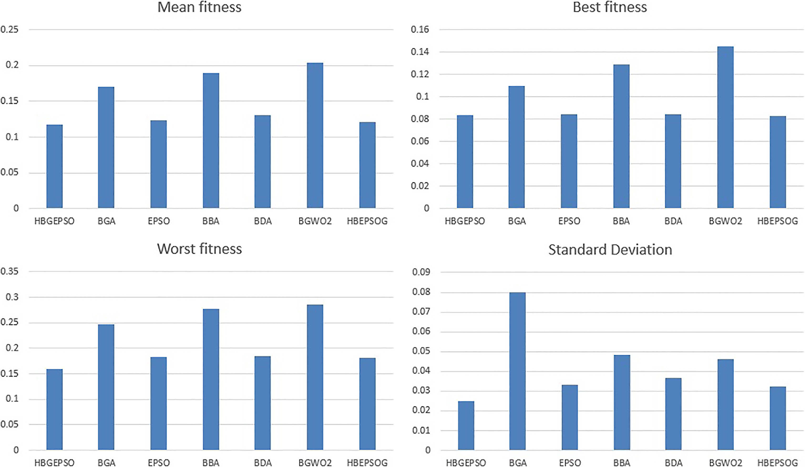
The Comparison of performance the HBGEPSO algorithm with other optimizers through main objectives of FS. The values are averaged over all the datasets.

Figure 2.

The Comparison of performance the HBGEPSO algorithm with other optimizers through few assessment indicators. The values are averaged over all the datasets.

7.1 Evaluation criteria

The datasets are divided into 3 sets of training, validation and testing. The algorithm is run repeatedly for $M=$ 10 times for statistical significance of the results. The following measures [16] are recorded from the validation data:

1.
Mean fitness function is the average of the fitness function value obtained from running the algorithm $M$ times. The Mean fitness function is calculated as shown in Eq. (12).

$\displaystyle\textit{Mean}=\frac{1}{M}\sum\limits_{i=1}^{M}{g_{i}^{}}$ (12)

where $g_{i}^{}$ is the best fitness value obtained at run $i$ .
2.
Best fitness function is the minimum of the fitness function value obtained from running the algorithm $M$ times. The Best fitness function is calculated as shown in Eq. (13).

$\displaystyle\textit{Best}=\min\limits_{i=1}^{M}{g_{i}^{}}$ (13)

where $g_{i}^{}$ is the best fitness value obtained at run $i$ .
3.
Worst fitness function is the maximum of the fitness function value obtained from running the algorithm $M$ times. The Worst fitness function is calculated as shown in Eq. (14).

$\displaystyle\textit{Worst}=\max\limits_{i=1}^{M}{g_{i}^{}}$ (14)

where $g_{i}^{}$ is the best fitness value obtained at run $i$ .
4.
Standard deviation gives the variation of the fitness function value obtained from running the algorithm $M$ times. It is an indicator of the stability and robustness of the algorithm. Larger values of standard deviation would suggest wandering results where as smaller value suggests the algorithm converges to the same value most of the times. The Standard deviation is calculated as shown in Eq. (15).

$\displaystyle\textit{Std}=\sqrt{\frac{1}{M-1}\sum\limits_{i=1}^{M}{(g_{i}^{}-% \textit{Mean})^{2}}}$ (15)

where $g_{i}^{}$ is the best fitness value obtained at run $i$ .
5.
Average Performance(CA) is the mean of the of the classification accuracy values when an algorithm is run $M$ times. The Average Performance is calculated as shown in Eq. (16).

$\displaystyle\textit{CA}=\frac{1}{M}\sum\limits_{i=1}^{M}{\textit{CA}^{i}}$ (16)

where $\textit{CA}^{i}$ is the Accuracy value obtained at run $i$
6.
Mean FS ratio(FSR) is the mean of the ratio of the number of selected features to the total number of features when an algorithm is run $M$ times. The Mean FS ratio is calculated as shown in Eq. (17).

$\displaystyle\textit{FSR}=\frac{1}{M}\sum\limits_{i=1}^{M}{\frac{\textit{size}% (g_{i}^{})}{D}}$ (17)

where $g_{i}^{}$ is the best fitness value obtained at run $i$ , $\textit{size}(g_{i}^{})$ gives the number of features selected and $D$ is the total number of features.
7.
Average F-score* is a measure that evaluates the performance of a chosen feature subset. It requires that in the data spanned by the feature combination the distance between data points in different classes be large and of those in the same class be as small as possible. The Fischer index for a given feature is calculated as in Eq. (18) [28].

$\displaystyle F_{j}=\frac{\sum\limits_{k=1}^{C}{n_{k}(\mu_{k}^{j}-\mu^{j})^{2}% }}{(\sigma_{j})^{2}}$ (18) $\displaystyle(\sigma_{j})^{2}=\sum\limits_{k=1}^{C}{n_{k}(\sigma_{k}^{j})^{2}}$ (19)

where $F_{j}$ is the fischer index for $j$ , $\mu^{j}$ is the mean of the entire data for feature $j$ , $(\sigma^{j})^{2}$ is defined as in Eq. (19), $n_{k}$ is the size of class $k$ , $\mu_{k}^{j}$ is the mean of class $k$ for feature $j$ , $(\sigma_{k}^{j})^{2}$ is the variance of class $k$ for feature $j$ . The Average F-score is calculated by taking the average of values obtained from $M$ runs for only the selected features.

7.2 Results

The proposed binary version of the HBGEPSO algorithm is compared with the binary GA, the Enhanced PSO, and other optimizers. The results are tabulated as follows.

Table 3 outlines the performance of the algorithms using the fitness function mentioned in Eq. (2) in the minimization mode. The table shows the average fitness obtained over $M$ runs and is calculated using Eq. (12). The best performance is achieved by the proposed binary version of the HBGEPSO algorithm proving its ability to search the feature space effectively.

Similar results are seen in Tables 4 and 5 that outline the best and the worst fitness function obtained over $M$ runs and is calculated using Eqs (13) and (14) respectively.

For testing the stability, robustness and the repeatability of convergence of these stochastic algorithms the standard deviation of the fitness values over $M$ runs is recorded as per Eq. (15) in Table 6. The table shows that the HBGEPSO algorithm can converge repeatedly irrespective of the random initialization.

The Best selected feature combinations by the algorithms are also allowed to run on the test data, and the average classification accuracy and the average FS ratio over $M$ runs is recorded using Eqs (16) and (17) respectively as shown in Eqs (7) and (8). As can be seen from these tables, the HBGEPSO algorithm can select the minimum number of features and yet maintain the classification accuracy. This shows the capability of the HBGEPSO algorithm to satisfy both the objectives of optimization.

To analyze the separability and closeness of the selected features Fischer score of these features is calculated as shown in Eq. (18). The average over $M$ runs is recorded in Table 9. As shown in the table, HBGEPSO algorithm achieves superior data compactness in comparison with the other algorithms.

These tables show that the HBGEPSO algorithm outperforms the other algorithms concerning all of the assessment indicators. It can also be seen that it performs much better when compared to its switched version HBEPSOG algorithm. This leads us to believe that the GA is powerful in exploring the search space and the enhanced PSO algorithm aids in exploiting the reduced feature space.

8. Conclusion

In this paper, a new hybrid binary metaheuristic algorithm with GA and Enhanced PSO algorithm is proposed in order to solve FS problems. The proposed algorithm is called Hybrid Binary Genetic Enhanced PSO(HBGEPSO) algorithm. The two algorithms come together to give better solutions that each of them individually. In order to verify the ruggedness and the effectiveness of the proposed algorithm, the proposed algorithm is applied on 20 FS problems. The evaluation is performed using a set of evaluation criteria to assess different aspects of the proposed technique. The experimental results show that the proposed method is promising with its ability to search the feature space effectively. The given algorithm was also run on test data, and observations show the higher performance of the selected features when compared to the other optimizers. The Fischer index table reveals better separability. It is also noted from the values of standard deviation that the algorithm has the robustness to repeatedly converge to similar solutions, therefore, a powerful ability to solve FS problems better than other algorithms in most cases.

Footnotes

Acknowledgments

This research was supported partially by Mitacs Canada. The research of the 1st author is supported in part by the Natural Sciences and Engineering Research Council of Canada (NSERC).

References

Agrafiotis

D.K.

and Cedeno

, Feature selection for structure-activity correlation using binary particle swarms, Journal of Medicinal Chemistry 45(5) (2002), 1098–1107.

Ali

A.F

and Tawhid

M.A.

, Hybrid bat algorithm and direct search methods for solving minimax problems, International Journal of Hybrid Intelligent Systems 14(4) (2018), 209–223.

Ali

A.F

and Tawhid

M.A.

, Hybrid particle swarm optimization with a modified arithmetical crossover for solving unconstrained optimization problems, INFOR: Information Systems and Operational Research 53(3) (2015), 125–141.

Banati

and Bajaj

, Fire fly based feature selection approach, IJCSI International Journal of Computer Science Issues 8(4) (2011), 473–480.

Bell

D.A.

and Wang

, A formalism for relevance and its application in feature subset selection, Machine Earning 41(2) (2000), 175–195.

Chandrashekar

and Sahin

, A survey on feature selection methods, Computers & Electrical Engineering 40(1) (2014), 16–28.

Chizi

Rokach

and Maimon

, A survey of feature selection techniques. Encyclopedia of Data Warehousing and Mining, seconded, IGI Global, 2009, pp. 1888–1895.

Chuang

L.Y.

Chang

H.W.

C.J.

and Yang

C.H.

, Improved binary PSO for feature selection using gene expression data, Comput Biol Chem 32 (2008), 29–38.

Coath

and Halgamuge

S.K.

, A comparison of constraint-handling methods for the application of particle swarm optimization to constrained nonlinear optimization problems, Proceedings of IEEE Congress on Evolutionary Computation 2003 (CEC 2003), Canbella, Australia, 2003, pp. 2419–2425.

10.

Coello Coello

C.A.

Luna

E.H.

and Aguirre

A.H.

, Use of particle swarm optimization to design combinational logic circuits, Lecture Notes in Computer Science (LNCS), No. 2606, 2003, pp. 398–409.

11.

Cotta

, A study of hybridisation techniques and their application to the design of evolutionary algorithms, AI Communications 11(3–4) (1998), 223–224.

12.

Eberhart

R.C.

and Kennedy

, A new optimizer using particle swarm theory, Proceedings of the Sixth International Symposium on Micromachine and Human Science, Nagoya, Japan, 1995, pp. 39–43.

13.

Das

A.K.

and Pratihar

D.K.

, Performance improvement of a genetic algorithm using a novel restart strategy with elitism principle, International Journal of Hybrid Intelligent Systems (2018), 1–15.

14.

De Jong

K.A

, Genetic algorithms: A 10 year perspective, In International Conference on Genetic Algorithms, 1985, pp. 169–177.

15.

Eberhart

R.C.

and Kennedy

, A new optimizer using particle swarm theory, Proceedings of the Sixth International Symposium on Micromachine and Human Science, Nagoya, Japan. 1995, pp. 39–43.

16.

Emary

Zawbaa

H.M.

Grosan

and Hassanien

A.E.

, Binary grey wolf optimization approaches for feature selection, Neurocomputing 172 (2016), 371–381.

17.

Frank

and Asuncion

, UCI Machine Learning Repository [http://archive.ics.uci.edu/ml]. Irvine, CA: University of School of Information and Computer Science, 2010.

18.

Goldberg

D.E.

, Genetic Algorithms in Search, Optimization, and Machine Learning, Addison-Wesley, 1989.

19.

Holland

J.H.

, Adaptation in Natural and Artificial Systems, University of Michigan Press, Ann Arbor, MI, 1975.

20.

Huang

Cai

and Xu

, A hybrid genetic algorithm for feature selection wrapper based on mutual information, Pattern Recognition Letters 28(13) (2007), 1825–1844.

21.

Kaya

, The effects of two new crossover operators on genetic algorithm performance, Applied Soft Computing 11(1) (2011), 881–890.

22.

Eberhart

R.C.

Shi

and Kennedy

, Swarm Intelligence (The Morgan Kaufmann Series in Evolutionary Computation), 2001.

23.

Khalid

, A survey of feature selection and feature extraction techniques in machine learning, Science and Information Conference (SAI), 2014.

24.

Krohling

R.A.

Knidel

and Shi

, Solving numerical equations of hydraulic problems using particle swarm optimization, Proceedings of the IEEE Congress on Evolutionary Computation (CEC 2002), Honolulu, Hawaii USA, 2002.

25.

Man

K.F.

Tang

and Kwong

, Genetic algorithms: concepts and applications (in engineering design), IEEE Transactions on Industrial Electronics 43(5) (1996), 519–534.

26.

Mirjalili

and Lewis

, S-shaped versus V-shaped transfer functions for binary particle swarm optimization, Swarm and Evolutionary Computation 9 (2013), 1–14.

27.

Nakamura

R.Y.

Pereira

L.A.

Costa

K.A.

Rodrigues

Papa

J.P.

and Yang

X.S

, BBA: a binary bat algorithm for feature selection. In 2012 25th SIBGRAPI Conference on Graphics, Patterns and Images, IEEE, 2012, pp. 291–297.

28.

and Han

, Generalized fisher score for feature selection, In Proc. of the 27th Conference on Uncertainty in Artificial Intelligence (UAI), Barcelona, Spain, 2012, arXiv preprint arXiv:12023725.

29.

Talbi

E.G.

, A taxonomy of hybrid metaheuristics, Journal of Heuristics 8(5) (2002), 541–565.

30.

Tawhid

M.A.

and Ali

A.F.

, A Hybrid grey wolf optimizer and genetic algorithm for minimizing potential energy function, Memetic Computing 9(4) (2017), 347–59.

31.

Tawhid

M.A.

and Ali

A.F.

, A hybrid social spider optimization and genetic algorithm for minimizing molecular potential energy function, Soft Computing 21(21) (2017), 6499–514.

32.

Tawhid

M.A.

and Ali

A.F.

, A simplex grey wolf optimizer for solving integer programming and minimax problems, Numerical Algebra, Control & Optimization 7(3) (2017), 301–23.

33.

Tawhid

M.A.

and Ali

A.F.

, Direct search firefly algorithm for solving global optimization problems, Applied Mathematics & Information Sciences 10(3) (2016), 841–860.

34.

Tawhid

M.A.

and Dsouza

K.B.

, Hybrid binary bat enhanced particle swarm optimization algorithm for solving feature selection problems, Applied Computing and Informatics (2018 Apr 11). https://doi.org/10.1016/j.aci.2018.04.001

35.

Tawhid

M.A.

and Dsouza

K.B.

, Hybrid binary dragonfly enhanced particle swarm optimization algorithm for solving feature selection problems, Mathematical Foundations of Computing 1(2) (2018), 181–200.

36.

Xue

Zhang

Browne

W.N.

and Yao

, A Survey on Evolutionary Computation Approaches to Feature Selection, IEEE Transaction on Evolutionary Computation 20(4) (2015), 606–626.

37.

Wolpert

D.H.

and Macready

W.G.

, No free lunch theorems for optimization, IEEE Transactions on Evolutionary Computation 1(1) (1997), 67–82.

Solving feature selection problem by hybrid binary genetic enhanced particle swarm optimization algorithm

Abstract

Keywords

1. Introduction

2. Definition of the feature selection problem

3.1 Main concepts and inspiration

3.2 Definition of concepts

4.1 Main concepts and inspiration

4.2 Movement of particles

7. Experimental results

Table 6 Standard deviation of the fitness function obtained from the different algorithms

8. Conclusion

Footnotes

Acknowledgments

References

Table 6
Standard deviation of the fitness function obtained from the different algorithms