EDGE: Evolutionary Directed Graph Ensembles

Abstract

This paper introduces Evolutionary Directed Graph Ensembles (EDGE). EDGE combines ideas from social dynamics and trust in human beings with graph theory. We use pre-trained prediction models as nodes in a directed acyclic graph where the connections between nodes have associated weight matrices to simulate the trust each node has in its predecessors. EDGE uses a genetic algorithm approach to evolve a population of these directed acyclic graphs, in an ensemble-type hybridization process. The pre-trained models are stored in a pool of models named Reservoir. The Reservoir can be populated with models from different families, such as Decision Trees, Ensemble Methods or Neural Networks. To test EDGE, four datasets were used: a dataset of a parking lot occupancy taken from a university student parking lot; a dataset about appliances energy use in a low energy building; a dataset of Anuran calls; and the MNIST dataset. Results show that we can achieve good accuracy measures of around 98% for the MNIST dataset, 99% for the Anuran data, 86% on the Appliances Energy and about 88% on the parking lot dataset. EDGE proves to be robust against bad performing nodes, presenting average accuracy results of up to 49% above the worst performing node in the ensemble. It also never shows results below the best performing node, and in some cases even improves the results with respect to the best node by up to 4%.

Keywords

Hybrid models ensemble methods genetic algorithms directed acyclic graph

1. Introduction

Currently we see prediction and classification problems being tackled in almost every scientific field, from cancer prediction[21] to credit scoring [1], classification of fake news headlines [30] and even predicting the effect of new combinations of drugs [19].

The idea of hybridization has also been extensively worked on, with applications ranging from prediction of properties of petroleum reservoirs [4] to assisting in photovoltaic (PV) panels modeling [27] and even frameworks for time series problems [29]. Its common feature is the desire to assimilate strengths from different models while mitigating their disadvantages, making for a more robust and powerful prediction tool. This work stems from that desire, and the idea of combining several models that influence each other, and where even worse performing models can be of use to help the system become more robust and target a wider range of patterns.

Inspired by previous work that focused on finding ways to hybridize models in search for better predictive performance, we developed Evolutionary Directed Graph Ensembles (EDGE) to a stage where it can be used in real world problems and extended to allow for a more general tool for common machine learning problems. EDGE picks up on the idea of hybridization by using a directed acyclic graph with a single sink for an ensemble of methods as well as having weights associated with the directed edges as a way to convey the trust of a node in its predecessors. EDGE brings about the evolution part of its name when evolving Directed Graph Ensembles as individuals of a population as well as incorporating different models in the ensembles.

In a previous work we presented a synthetic dataset representing the occupancy rate of a student parking lot throughout the year, which was used to test different approaches as possible base models [11]. This dataset represents a time series instance with the caveat that we discretized the output into several classes. From the different approaches that were tested, and after some parameter tuning, three worked best: Decision Trees (DTs), Random Forests (RFs) and Gradient Boosting models (GBs). In another work, three additional datasets were used for comparison, also with the intent of assessing whether or not some proposed hybrid approaches had more predictive power than the base models used in the hybrid [12].

This paper builds on that work, further refining and formalizing the most promising model – EDGE – and testing its capabilities using datasets with different characteristics.

The rest of this paper is organized as follows. In Section 2 we discuss some works that also use ensembles, hybrid approaches and evolutionary algorithms. Section 3 introduces some previous work in hybrid prediction models, as well as the parking lot dataset. Section 4 presents a formal definition of EDGE and its inner workings, as well as some constraints and assumptions. The experimental setup is outlined in Section 5 and its results are presented and discussed in Section 6. In Section 7 we present some conclusions regarding this work and in Section 8 we describe some of the future developments planned for EDGE.

2. State of the art

Hybrid approaches stem from the idea of joining advantages of the models they are based on, while mitigating their disadvantages. Having in mind the context of this work, in the following sections we focus on analyzing ensemble methods, hybrid prediction models and evolutionary algorithms to give a sense of common approaches and current work in these domains.

2.1 Ensemble methods

Two of the most commonly used ensemble methods are Random Forests and Gradient Boosting models. In [32] several ensemble methods are compared and studied. Some of the most recent methods for ensemble generation are Bagging (of which RFs are an example) and Boosting (GBs for example). Bagging is used to reduce the variance of an estimated prediction function while Boosting relies on the idea of modifying weak learners [3].

Random Forests rely on the idea of averaging out possible mistakes by building a large collection of de-correlated trees [18]. In the context of time series regression, RFs were used to deal with weekly influenza-like illness rate prediction, achieving Mean Absolute Percentage Error (MAPE) of about 4% [43].

GB models have been used by Johnson et al. for predicting waste patterns [22]. The authors used several datasets from New York City in conjunction with historical municipal solid waste (MSW) data to predict patterns in MSW and catch short timescale fluctuations. GBs were also used in [46] for travel time prediction with real-world traffic and sensors data.

Despite the frequent use of Decision Trees (DTs) as baseline model for the ensembles, others can be used, such as Neural Networks (NNs) or Support Vector Machines (SVMs). An ensemble of SVMs was proposed by Kim et al. with bagging or boosting [24]. This ensemble was tested on three datasets and was shown to outperform single SVM instances. On the IRIS and UCI hand-written digits datasets the improvement was of about 2 percentage points while the results for fraud detection saw an improvement of about 5 percent.

In [2] two tree-based ensemble methods were used to predict photovoltaic power generation and compared with Support Vector Regression (SVR). The two ensembles were Extra Trees (ETs, also called Extremely Randomised Trees) and RFs. Assessing the performance using Root Mean Squared Error (RMSE), Mean Absolute Error (MAE) and the determination coefficient $R^{2}$ and doing hyper-parameter tuning, the ETs method was shown to perform at the same levels of RF with an accuracy of 92% and both of these to outperform SVR with an accuracy of 90%.

Ensemble learning was used in [36] for malware detection at the hardware level. This is a binary classification problem where processor Hardware Performance Counters (HPCs) data was fed to several methods and their performance compared. The work shows ensemble learning through Bagging and using a Boosting technique, AdaBoost [13] and other classifiers such as Stochastic Gradient Descent (SGD) and Bayesian Networks. Experimental results showed that ensemble methods outperformed standard classifiers by up to 17% while using less HPCs.

Torres-Barrán et al. tested GBs, RFs and Extreme Gradient Boosting (XGB) to model two problems, wind energy and solar radiation [41]. The experiments included an exploration of the parameter space state and results were compared with the ones of SVR models and Multilayer Perceptrons (MLPs). Although no method distinguished itself from the others, the results point out that ensemble methods rival the performance of more contemporary methods used in Machine Learning.

In the context of classifying data streams, one of the most challenging tasks of data stream mining, Zhang et al. present a new type of data structure, Ensemble-Tree (E-Tree) Indexing Structure, for high speed stream records, achieving sub-linear prediction [45]. The authors propose four different variants of the ensemble method and use them for online search label comparisons. When comparing E-Tree with single trees, the conclusion was that while the test time was bigger for the ensemble, the error rates dropped from 1.5% on the tree to 1.2% on the ensemble.

To showcase another domain where ensemble methods have been tried out, we can cite the work of Hu et al., who used RFs and XGB, as well as SVMs as base models for ensembles to predict lncRNA protein interactions [20]. The models were experimented on different features from the lncRNA and from the protein in study and the sub models were also evaluated to see if the ensembles performed better than the base models. The conclusion was that the proposed ensembles had better predictive performance than the standalone models and even than other proposed models. Similarly, Simopoulos et al. used RFs and Stochastic Gradient Boosting classifiers as elements of a single stacking meta-learner and several ensemble types were proposed and evaluated [38]. The authors concluded that the use of an ensemble approach increased the power of the models and the opportunity to use different models, combining their strengths.

2.2 Hybrid models

Very often we see the combination of models as a way to couple models which are good at predicting the linear component of the data with models that perform better at the non-linearity prediction. An example of this is the combination of Autoregressive Integrated Moving Average (ARIMA) with Artificial Neural Networks (ANNs) made by Zhang, using the ARIMA to predict the linear component and the ANN the nonlinear component. This combination was experimented on three datasets with the hybrid competing against its base parts and the results showed a clear victory for the hybrid when considering the error of each model [44].

Pai and Lin use ARIMA as well, but in conjunction with an SVM model. The ARIMA model is used for the linear component of the data, while the SVM is used on the residuals, which comprehend the non-linear component of the data. Tested on forecasting daily closing stock prices, the hybrid was compared to the ARIMA and SVM models. The results showed that the hybrid model can reduce forecasting errors. Also an interesting conclusion is that not always do the best configurations, when considering the standalone models, translate into the best performing hybrid, which may point to the fact that hybrids might benefit more from base models that are somehow complementary of each other[33].

An attempt at predicting bankruptcy with the integration of genetic algorithms (GA) and SVM is presented by Min et al. where the performance of the SVM is improved by using GA for feature selection and parameter optimization. The hybrid GA-SVM model is presented with three variants – one that optimizes the feature subset to be used in the SVM; a second that optimizes the parameter selection using GA on the kernel function’s parameters; and a third that does both parameter and feature selection optimization. Focusing on improving the SVM, the work showed that the approach had success in improving SVM prediction power and that the feature selection influenced how the parameter choice would favor the performance of the model [31].

We can also see works where the models are more deeply integrated, such as in [15] where we see a combination between Multi-dimensional Bayesian Network Classifiers (MBCs) and classification trees, named Multi-dimensional Bayesian Network Classifier Tree (MBCTree). This approach is similar to [25], where a hybrid between Naive Bayes classifier and a Decision Tree was proposed, Naive Bayes tree (NBTree). The proposed MBCTree is a classification tree with MBCs in the leaves, where an internal node corresponds to a feature variable and a leaf node corresponds to a MBC over all the class variables and feature variables not present in the path from the root to the leaf. The experiments, conducted on synthetic datasets, showed that the MBCTree achieved better accuracy than the MBC model, especially in cases when the data was generated from more disparate probability distributions.

More recently, three different hybrids were presented by Koopialipoor et al. [26]. The three variations used ANNs to predict an adverse side effect produced by blasting mines and tunneling projects, flyrock distance. To adjust the weights and biases of the ANN three approaches were used: Imperialist Competitive Algorithm (ICA), GA and Particle Swarm Optimization (PSO). The models were evaluated on two performance indices, RMSE and $R^{2}$ . Results showed that although all variants displayed acceptable predictive performance, the PSO-ANN distinguished itself from the other two. The results were also compared to previous work on the same dataset and the hybrids managed better results. This type of hybrids are mentioned in [16].

As mentioned in Section 2.1, there are also hybrid works in the context of medical sciences. In the ensemble type of hybrids, a more robust method for brain tumor segmentation is experimented, the Ensembles of Multiple Models and Architectures (EMMA) [23]. The ensemble consisted of a heterogeneous collection of CNNs to make a system insensitive to independent failures that generalizes well. It’s worth noting that EMMA won first place of a brain tumor segmentation challenge.

In [17] hybrid models are used to simulate static and dynamic behaviour of gears. This is done by combining sub-structures of different models to better simulate the behaviour of high-speed thin-rimmed gears. The results from comparing this approach with numerical results proves its versatility and capacity to simulate actual gear sets.

We can see that it is a relatively common approach to use one method to find the best configuration of another in a given prediction task. There are also works where two different models are integrated with one another and even works were an ensemble of different methods is used. There is a multitude of hybridization proposals in search of better performance.

2.3 Evolutionary algorithms

One key area of evolutionary algorithms (EAs) have been used is in multiobjective optimization (MO), this is, a problem where we try to optimize more than one objective function. In practice these objective functions collide with each other and a consensus must be reached and the usual population-based nature of EAs allows us to get several non-dominated solutions [5]. We would also like to reference two surveys made of EAs when applied to MO, usually referred to as MOEAs [42, 35].

From Section 2.2 we can see that many works incorporating EAs use these methods to improve on the performance of other models, such as ANNs, SVMs, etc. In [40], a classifier is presented as a way to maximize profit when modeling customer churn rates, by using genetic algorithms (GAs).

On the topic of protein prediction, in [14] an EA designed for multiobjective optimization is presented to predict the three-dimensional structure of proteins from their one-dimensional sequence. The approach relies on establishing three objective functions and comparing it with prior methods, observing that this approach improves or rivals prior approaches and formulations of the same problem that take only into account two objective functions.

On their application to graphs, EAs have been used to tackle problems that can be formulated as graphs [6, 10] and incorporated with graphs as a way to devise new EAs [28]. In [6] EAs are used for graph partitioning problems, more precisely on balanced k-way partitioning of graphs. On the other side, the same type of algorithms are used in [10] for the k-coloring problem, this is, coloring every node of a graph using one of k colors such that no adjacent nodes share the same color. GNP (Genetic Network Programming) is a graph-based evolutionary algorithm with the intent of improving performance on dynamic environments due to the expression ability of graph structures [28].

The idea of evolving topology has also been used in [39] with the evolution of neural networks through a method called NeuroEvolution of Augmented Topologies (NEAT). Experiments were made on the Pole Balancing and Double Pole Balancing problems. The results showed that NEAT manages to evolve the structure of the network when necessary and provided better results while finding more minimal solutions. It’s also a robust method, being less likely to get stuck on local solutions.

In [34] genetic algorithms are used for community detection in graphs. Detecting a community means detecting nodes that share some form of similarity between them while at the same time having a high degree of connections between them. Compared with other algorithms for community detection on five synthetic datasets, it was shown that this proposal rivals that of prior work and is able to exploit both the attributes of the nodes and the structure of the graph.

3. Previous work

The idea behind EDGE was briefly introduced in [11], where we tackled the task of predicting the occupancy rate of a university student parking lot. For that, we gathered data from several sources: the parking administration provided us with schedules for student classes and exams, as well as all recorded accesses to the park (entrances and exits); from the internet we gathered national and regional holidays for the municipality where the parking lot is located; and from a public API2 of a weather station located about 800 meters from the parking lot we obtained information such as temperature, rain, humidity or wind chill, among others, in intervals of 5 minutes.

When processing the park access records, we noticed some inconsistencies, such as students entering or exiting the park several times in a row, as well as long time intervals with no registered access data. As this data was much too noisy and contained several problems, we took the opportunity to generate an artificial version of the dataset after modeling the parking lot using knowledge from the system administration, weather and holiday information, the park’s maximum capacity and actual student class enrollments, schedules and exams. The target variable (occupancy rate) was discretized into 10 classes, each representing an interval for the occupancy rate of the park. This division allowed us to catch situations where the park is almost full (intervals [80%, 90%] and [90%, 100%]), almost empty (intervals [0%, 10%] and [10%, 20%]) plus everything in between.

Using this data we tested five different models – DTs, GBs, RFs, Convolutional NNs (CNNs) and Long Short-Term Memory Networks (LSTMs) – with some hyper-parameter tuning. This choice of models to use came from a literature review where several models were studied, their strengths, weaknesses and works where their use produced good results. The three best performing methods were the DT, RF and GB. It is interesting to note that the top performing models were tree based and that LSTMs performed worse than expected, leading us to conclude that maybe the configurations used for the neural networks were not the most appropriate.

Figure 1.

EDGE architectural diagram.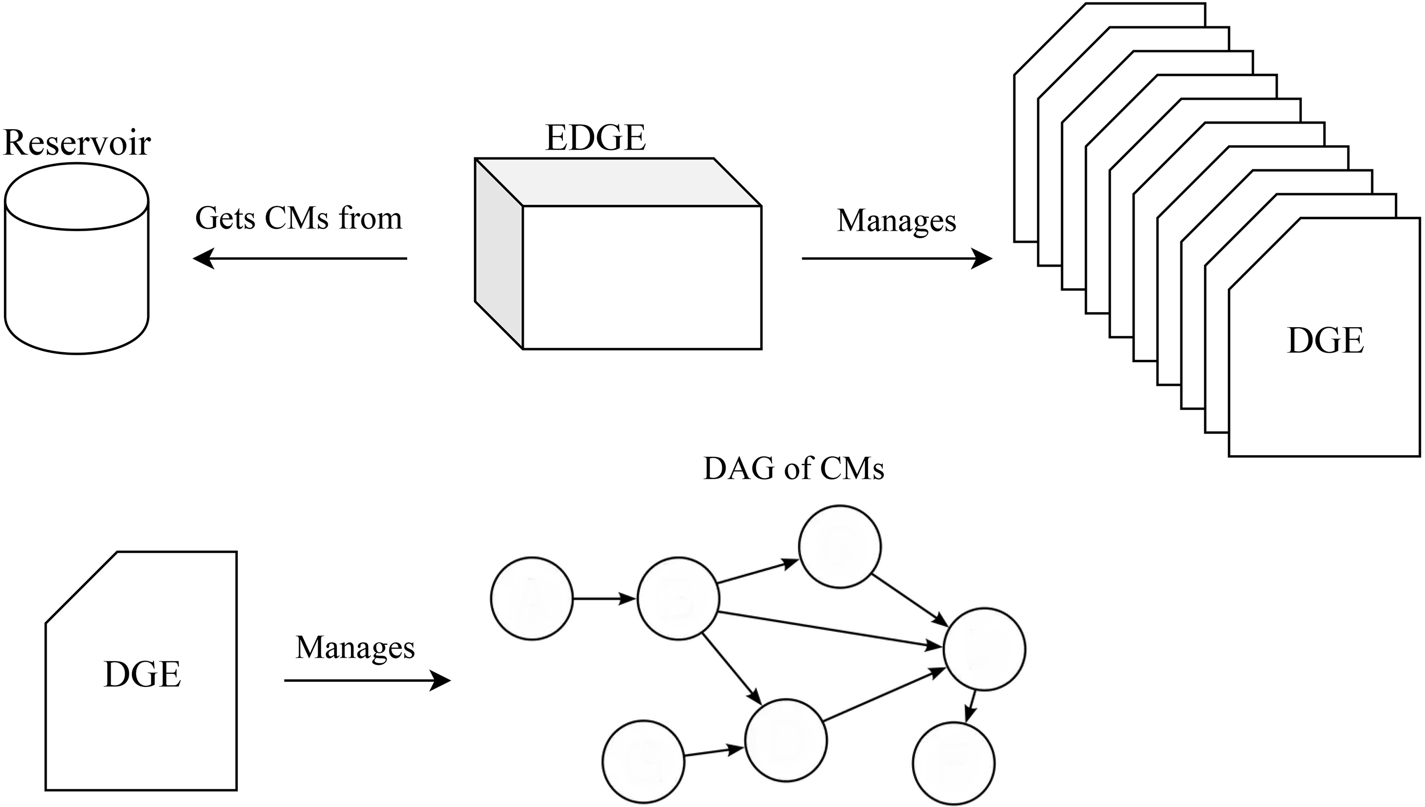

The DT, RF and GB were later used to explore possible approaches to combine the different models [12]. Three approaches for hybridization were proposed: one based on voting mechanisms; one based on pairs; and one based on social trust, a primitive version of EDGE. The voting approach relied on three models and a voting system that operated with different policies to evaluate which gave better results. The pair hybrid combined the predictions of a first model when feeding the input to a second model; the idea was to have the second model figuring out when the first model made a wrong prediction and answer accordingly. The third one was a primordial version of EDGE, which consisted of only one DGE with a fixed, user-defined, structure The models used as the building blocks for these hybrids were the three models found to have better performance on the previous work (DTs, RFs and GBs). These building blocks were followed by some hyper-parameter tuning and tested on more datasets to empirically verify if any of the approaches had potential to improve prediction performance.

From the previous works we gathered the idea for EDGE; models that appear to be strongly suited for the parking lot dataset; and the dataset itself, which represents a time series with non-periodic external factors. The focus now is on proving that EDGE can increase the prediction power against its basic methods, while being robust enough to work well even when the DGE’s base models are not particularly good.

4. EDGE formulation

EDGE manages and applies a genetic algorithm approach to grow its population of Directed Graph Ensembles (DGEs). Each DGE is represented as a Directed Acyclic Graph (DAG) with the constraint of having only one sink node. A brief diagram of the system’s architecture is presented in Fig. 1. EDGE brings the idea of trust in a social environment to a predictive model scenario. This is achieved by evolving several DGEs, which represent a given network of nodes that have weights associated to other nodes in which they trust. These nodes are standalone models, what we call Component Models (CMs), and are randomly sampled from the Reservoir, a structure that acts as a resource pool for all types of model-configuration pairs that can be used.

4.1 Reservoir

When setting the stage for EDGE, we need to set up an auxiliary data structure, the Reservoir. This data structure is fed a specification of a type of model and the range of parameter values, i.e., its desired configuration space. The Reservoir can also be fed with proper models, already configured. When needed, the Reservoir returns a random model based on its internal models and specifications plus configuration space. The desired configuration space is set up by the user and can be arbitrarily large. It’s worth noting that all possible combinations have equal probability of being chosen.

4.2 DGEs

The nodes of the DGE mentioned above as Component Models (CMs) are full-fledged standalone models such as the type of models used in regular prediction problems. The edges of the DGE represent the flow of information through the DAG until the sink node and are associated with weights corresponding to each node’s trust in its predecessors. The CMs are supplied by the Reservoir.

Let $X_{j}$ denote a generic feature vector $j$ of the dataset and $Y_{j}$ denote the corresponding target attribute. Let $\textit{CM}_{i}$ represent a given Component Model $i$ . We are assuming the Component Models are properly trained and can be used to predict $Y_{j}$ from a data point $X_{j}$ . We model $\textit{CM}_{i}$ such that $\textit{CM}_{i}(X_{j})=Y_{j}\prime$ where $Y_{j}\prime$ is a vector with the probability for each class, in case of a classification task; or a scalar denoting the value of the predicted target attribute, in case of regression problems. Each CM has also a scalar $\alpha$ that represents its self-confidence.

Let a DGE be represented as a graph $G=(V,E)$ where $V$ denotes its vertices (or nodes) and $E$ its edges. The constraints on $G$ are as follows:

•
$G$ is a DAG;
•
$\exists_{=1}\ v\in V$ such that $v$ has only incoming edges (there is exactly one sink);
•
$\forall v\in V$ there is at least an edge $(u,t)\in E$ such that $v=u\lor v=t$ (there are no isolated nodes).

The goal of the DGE is to use its structure to predict a given data point. For this and to make sure we propagate the predictions of a vertex to its successors, we need to go through the vertices following a topological ordering.

Each node of the DGE performs the same process to give its prediction about a given data point, except for the nodes that have no incoming edges. For the nodes without incoming edges the prediction they pass along their outgoing edges is simply the prediction of its CM. For every other node we use the following formula:

$\displaystyle P_{i}(X_{j})=\alpha\times sp_{i}(X_{j})+(1-\alpha)\times\frac{pp% _{i}(X_{j})}{\|pp_{i}(X_{j})\|}$

Where

$\displaystyle pp_{i}(X)=\sum_{n\in\textit{predecessors(i)}}\frac{P_{n}(X)\circ W% _{i}^{n}}{\|P_{n}(X)\circ W_{i}^{n}\|}$

Considering that:

•
$\circ$ represents the Hadamard product, also known as element-wise or point-wise multiplication.
•
$sp_{i}(X)$ , for self-prediction, denotes the prediction made by $CM_{i}$ .
•
$pp_{i}(X)$ , predecessors prediction, denotes the sum of the predictions of the predecessors of node $i$ .
•
$W_{i}^{n}$ represents the trust vector of node $i$ in its predecessor, node $n$ .
•
The normalization is used in both types of problems (classification and regression). However, the formula can be tweaked to suit specific needs; for instance, in regression we might only normalize the trust in the predecessors to make sure their weights sum up to 1, constraining the range of weights to the interval [0, 1].

The $W$ factor is bootstrapped using a sample of the dataset the CMs have never seen, and then calculating the recall score. Note that other ways are possible such as the precision score or F-beta score. We believe this approach makes for a better starting point than just initializing $W$ with random values. At the same time, the sample used to bootstrap is one the models have not seen and as such we believe it is a good estimate of real performance as opposed to using the same data the models were trained with.

To summarize the DGE, from the perspective of a node in its structure, we take into account the prediction of a given data point and the predictions of the predecessors where each predecessor is associated with a given trust. The fact that the trust is a vector in classification tasks means we can trust a predecessor only when it predicts a given subset of the target classes, thus making this method a very promising one when dealing with specialized classifiers.
4.3 EDGE

Each DGE represents an individual in a population Pop of size PopSize. We define NElite as a user-defined value representing the number of top-ranking individuals to keep from one generation to the next and NBottom as a number representing how many new DGEs to create between generations as a way to introduce substitutes for the worst performing individuals, while also promoting the exploration of new solutions.

We build the initial population by creating PopSize DGEs with only two nodes and applying a random mutation to them so that the basic building block of the DGEs is a simple structure, as seen in Fig. 2.

Figure 2.

Basic Structure of a DGE.

We evolve the population by performing a generation step, which can be of one of two kinds: topology-based or trust-based. In a trust-based generation step we evolve the trust matrices that connect each node to its predecessors. In a topology-based generation step we evolve the topology of the DGE.

To perform a trust-based step we need to take the trust matrices of each node and calculate the gradient, similarly to what is done in neural networks. From our analogy with social networks, we also must take into account the confidence each node has in itself and as such this calculated gradient must also take into account a node’s own predictions. This trust-based step can also result in actionable insights. For instance, we could cut the connection with a predecessor if the trust in it is below a certain threshold, with the rationale that the predecessor is not contributing enough for the node’s predictions.

Each topology-based step follows 4 ordered sub-steps:

Evaluate the population;

Save the top $N E l i t e$ DGEs;

Cross the population to generate child DGEs;

Mutate the child DGEs.

Sub-step 1 requires only that the user specifies a function to be used to evaluate the performance of any given DGE. This function should be in the form of $f(\textit{DGE}_{i},X_{\textit{eval}},Y_{\textit{eval}})$ where the return value is a fitness indicator of how good the solution is, ie, a distance measure between $Y_{\textit{eval}}$ and the result of applying $\textit{DGE}_{i}$ to $X_{\textit{eval}}$ . $X_{\textit{eval}}$ and $Y_{\textit{eval}}$ are vectors of data points and corresponding targets to evaluate the DGE.

Sub-step 2 saves the best performing DGEs to advance to the next generation without change. This step also includes an optional integer parameter NBottom where NBottom DGEs are generated from scratch as a way to introduce some new individuals into the population, favouring exploration of new random DGEs.

Sub-step 3 needs to create $\textit{PopSize}-\textit{NElite}-\textit{NBottom}$ children DGEs to complete the population. To do so, we choose any two DGEs from the previous population where the probability of any DGE being chosen is proportional to its evaluation score. The two selected DGEs are crossed using a user-defined heuristic such that from two DGEs we obtain possible children. In a generic way, it should be a function $\textit{cross}(\textit{DGE}_{i},\textit{DGE}_{j})$ that returns the result from crossing $\textit{DGE}_{i}$ with $\textit{DGE}_{j}$ , two children DGEs. We suggest a division in the topology in two subgraphs for each DGE such that two child DGEs can be created by combining a subgraph from $\textit{DGE}_{i}$ with another from $\textit{DGE}_{j}$ .

Sub-step 4 mutates the children DGEs obtained from sub-step 3. There are 5 equally likely mutations to occur on the structure of the DGE:

•

Delete a random edge from the DGE;

•

Add a random edge between two existing nodes;

•

Delete a random node and any adjacent edges;

•

Add a random node to the DGE, which implies adding an edge; we propose adding an edge from the new node to one of the other nodes;

•

Swap any two nodes.

Mutations are constrained so that their results are guaranteed to being weakly connected DAGs with only one sink. Other suggestions we propose as more complex mutations would be to evaluate the graph structure and merge several nodes into one or split one node into various, creating and deleting the appropriate connections. One possibility interesting mutation would be to discover network motifs [37] and switch them in the graph structure, nodes and associated trusts.

We apply NGenerationsalling of the anurans. The steps as described above. To further customize the evolution process, the user may define the type of step to be performed at each generation or a ratio representing how many trust-based steps to perform for each topology-based step.

With this we complete our formulation of EDGE, its components and its inner workings. It’s worth noting that our formulation doesn’t restrict EDGE’s extensibility and customization.

5. Experimental setup

We start by introducing the datasets used in the experiments, explaining which were used, what kind of transformations were done and the reasons for these choices. As for the experiments, we first perform tests on static DGEs and then with evolving DGEs. On the evolving DGEs we first fill the Reservoir with DTs alone, and then we fill it with DTs, RFs and GBs.

5.1 Datasets

The Anuran dataset [8] and the MNIST dataset [9] represent classification tasks. The Anuran dataset has Mel-frequency cepstral coefficients (MFCCs) as feature variables that are to be used to predict the species of anuran. These coefficients collectively represent the short-term power spectrum of a sound, in this case, the calling of the anurans. MNIST is a well-known dataset used in benchmarking classification tasks where images of hand-written digits are labeled with the corresponding digit. These datasets both have 10 target classes but while the Anuran dataset uses numeric coefficients as features, the MNIST uses images, so they are good candidates for a varied test sample.

Figure 3.

DGE with 3 nodes (pred. – prediction).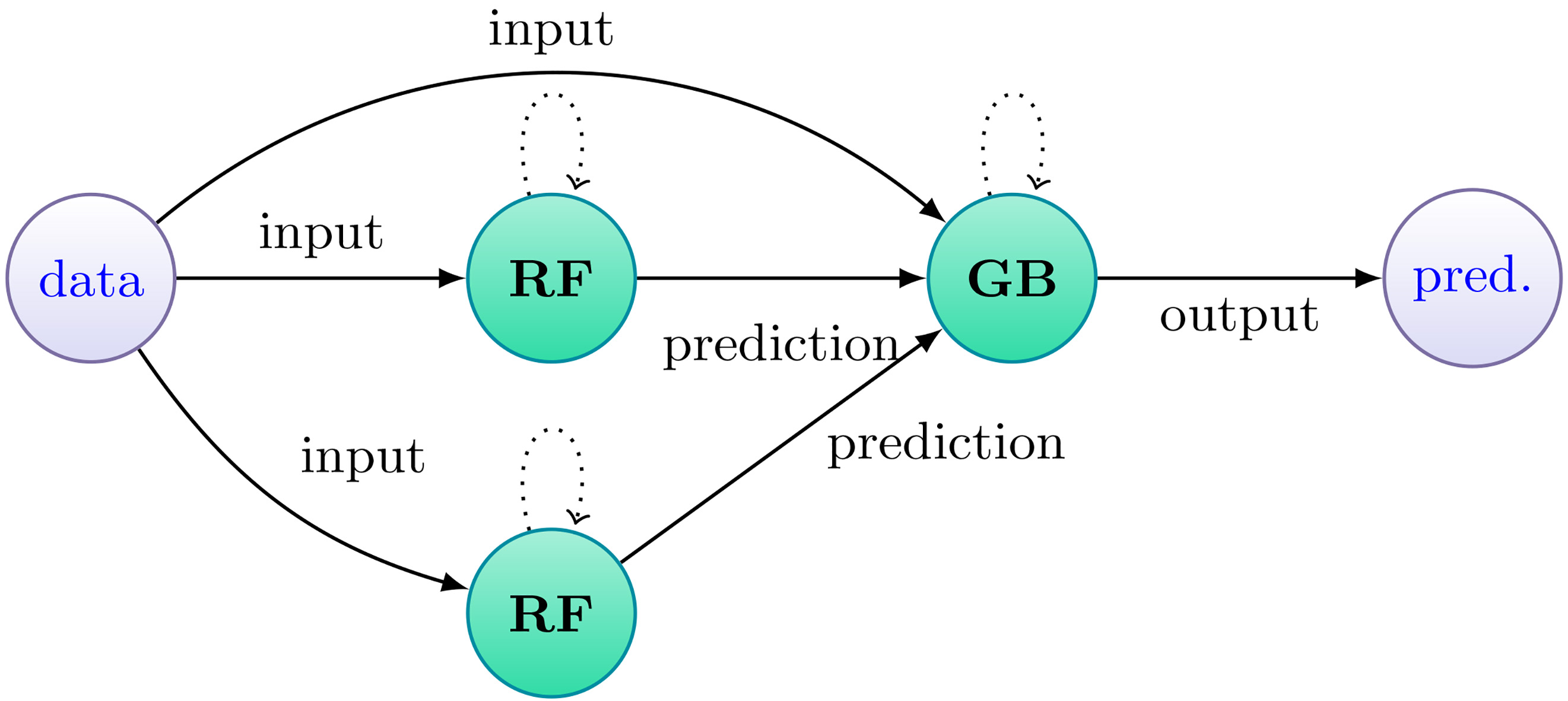

To also use regression data we decided to use the Parking Lot and the Appliances Energy dataset [7]. At the time of writing, EDGE doesn’t yet include regression capabilities, so we decided to discretize both regression datasets into 10 classes, the same number as the classification datasets, so as to have some common ground among all datasets. They were chosen for being representatives of time series. The Parking Lot dataset has features that represent external stimuli like holidays and weather information. The Appliances Energy dataset is an example of a time series where we have one target value to be predicted, in this case appliances energy use in a low energy building.

5.2 Static DGEs

Initially, we followed a more basic approach of forcing a topology without the evolutionary component being involved, to verify whether or not the DGEs prediction capabilities improved when compared to its base models. We experimented with different topology settings, number of nodes and edges between them. In Fig. 3 we present the diagram of a simpler DGE and in Fig. 4 we showcase a more complex topology. All the tests were run 10 times and their metrics averaged. The models used and their parameters are shown in Table 1.

Table 1
Parameters of base models for static DGEs

Parameter	GB	RF
Training examples (%)	80	80
Estimators	5	100
Criterion	Mean squared error	Gini impurity
Max depth	100	100
Max features	All features	All features
Learning rate	0.01
Loss	Deviance

Table 2

Parameter combinations of Reservoir for Evolving DGEs – first experiment

Parameter	DT values
Training examples (%)	80
Criterion	Info. gain
	Gini impurity
Splitter	Best, random
Max depth	5, 10, 15, 20
	50, 100, 500, 1000
Max features	All features, sqrt
	Log2, 33%, 50%, 66%
Min samples split	2, 4, 8, 16

Figure 4.

DGE with 5 nodes. Text on prediction edges was omitted. (pred. – prediction).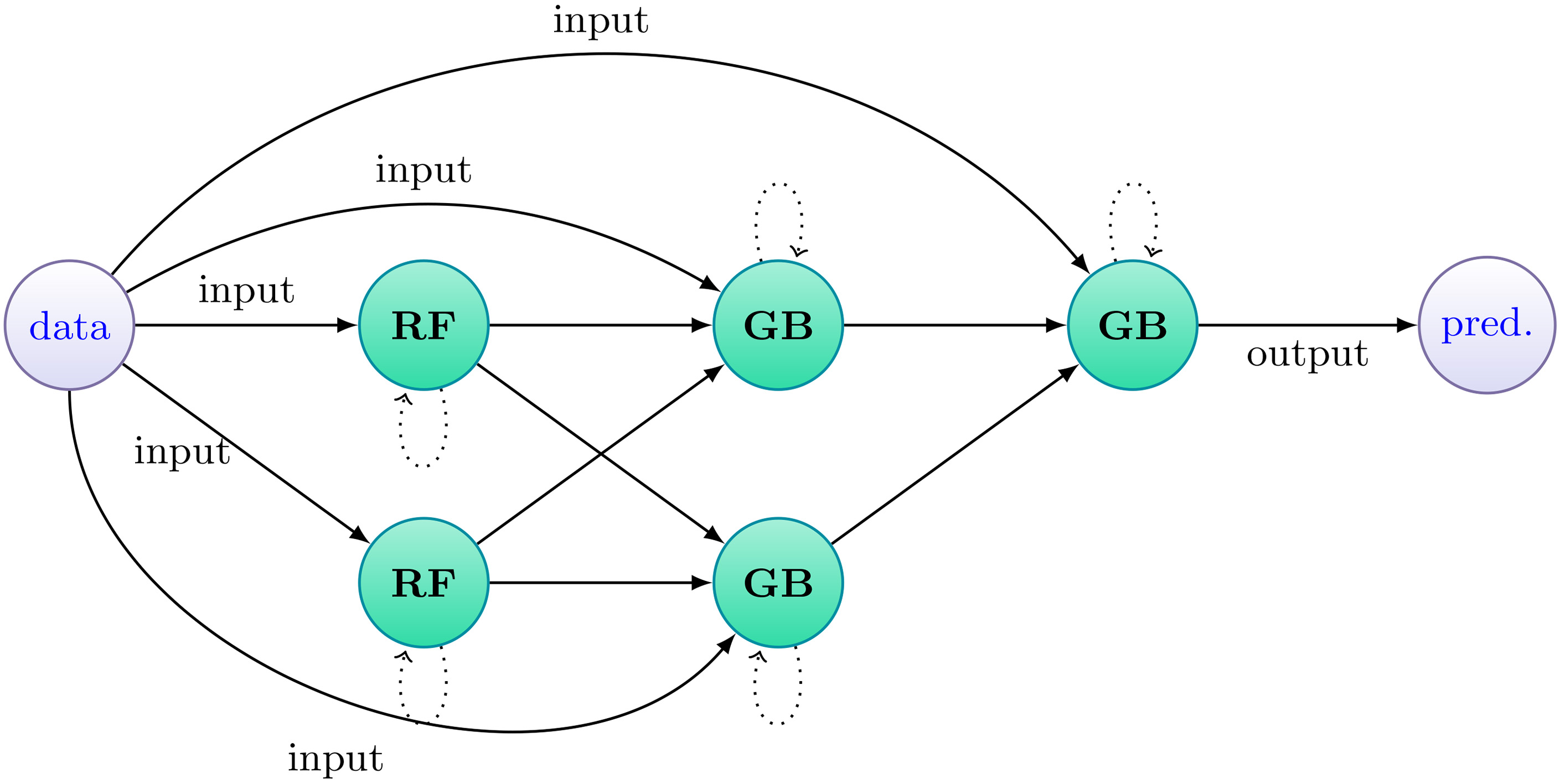

Table 3

Parameter combinations of Reservoir for Evolving DGEs – second experiment

Parameter	GB	RF	DT
Training examples (%)	80	80	80
Estimators	5, 10, 15, 20	10, 50, 100, 200
	MSE	Info. Gain	Info. Gain
Criterion	Friedman MSE	Gini impurity	Gini impurity
Max depth	10, 100, 200	10, 100, 200	10, 50, 100, 1000
Max features	All features	All features	All features
		Sqrt	Sqrt, Log2
Learning rate	0.01, 0.1
Loss	Deviance
Splitter			Best, random

5.3 Evolving DGEs

For this test stage, we decided to first fill the Reservoir with DTs only, as they are one of the most used model when building ensembles. Also, since they are not as time-consuming as other methods, we can also expedite these initial EDGE tests before advancing to experiments with different models. For the first experiment, we filled the Reservoir with DTs from the configuration space presented in Table 2.

For the second stage of experiments, we filled the Reservoir with the three models previously selected, namely DT, RF and GB, using the configurations presented in Table 3.

Note that the combinations revolve around the configurations presented in Section 5.2. It should also be noted that, as the time of writing, we are not evolving the trust of each node in its predecessors, as mentioned in Section 8 but only the topology of the DAG. Even though we believe both steps could provide for better performance, this allows us to isolate and better analyze the contribution of each step to EDGE’s global performance.

Table 4
Parameter values for EDGE configuration

Parameter	Value
NElite	2
NBottom	0
PopSize	20
NGenerations	100

The crossing heuristic used, a necessary step mentioned in Section 4.3, was implemented in a way that crossing two DGEs returns two children. A pseudocode for this algorithm is presented in Algorithm 5.3. The general idea for this algorithm is to break each DGE’s graph structure into two subgraphs such that they can combine with the two subgraphs from another DGE. For clarification purposes, mentions to left and right in the algorithm are considering a horizontal visualization of the graph, with the sources to the left and sink to the right.

Crossing algorithm used in experiment $\textit{DGE}_{i}$ , $\textit{DGE}_{j}$ $\textit{DGE}_{m}$ , $\textit{DGE}_{n}$ Fcombinecombine Fdividedivide_topology

FnFunction: DGE $\textit{sorted\_nodes}=\textit{get\_topological\_order(DGE)}$ $\textit{nodes}_{\textit{left}}=[]$ $\textit{nodes}_{\textit{right}}=[]$ $\textit{size(sorted\_nodes)}\%2==0$ $\textit{nodes}_{\textit{left}}=\textit{first\_half(sorted\_nodes)}$ $\textit{nodes}_{\textit{right}}=\textit{second\_half(sorted\_nodes)}$ $\textit{nodes}_{\textit{left}}=\textit{all\_before\_middle(sorted\_nodes)}$ $\textit{nodes}_{\textit{right}}=\textit{all\_after\_middle(sorted\_nodes)}$ $\textit{middle\_node}=\textit{get\_middle(sorted\_nodes)}$ $\textit{in\_degree(middle\_node)}<=\textit{out\_degree(middle\_node)}$ $\textit{nodes}_{\textit{left}}.\textit{append(middle\_node)}$ $\textit{nodes}_{\textit{right}}.\textit{append(middle\_node)}$ $\textit{subG}_{\textit{left}}=\textit{subgraph\_from\_nodes(DGE, nodes}_{% \textit{left}})$ $\textit{subG}_{\textit{right}}=\textit{subgraph\_from\_nodes(DGE, nodes}_{% \textit{right}})$ $\textit{subG}_{\textit{left}}$ , $\textit{subG}_{\textit{right}}$ $G_{\textit{left}}$ , $G_{\textit{right}}$ $g=\textit{graph\_union}(G_{\textit{left}},G_{\textit{right}})$ $\textit{node}_{l}\in\textit{get\_sink\_nodes}(G_{\textit{left}})$ $\textit{node}_{r}\in\textit{get\_source\_nodes}(G_{\textit{right}})$ $\textit{g.add\_edge}(\textit{node}_{l},\textit{node}_{r})$ $g$ $\textit{sub\_graph}^{i}_{\textit{left}},\textit{sub\_graph}^{i}_{\textit{right% }}=\textit{divide\_topology}(\textit{DGE}_{i})$ $\textit{sub\_graph}^{j}_{\textit{left}},\textit{sub\_graph}^{j}_{\textit{right% }}=\textit{divide\_topology}(\textit{DGE}_{j})$ $\textit{DGE}_{m}=\textit{combine}(\textit{sub\_graph}^{i}_{\textit{left}},% \enskip\textit{sub\_graph}^{j}_{\textit{right}})$ $\textit{DGE}_{n}=\textit{combine}(\textit{sub\_graph}^{j}_{\textit{left}},% \enskip\textit{sub\_graph}^{i}_{\textit{right}})$

As for the parameters of the EDGE, as mentioned in Section 4, we present their values in Table 4. The reason for such arguably small values is due to time-constraints. Nevertheless, it’s worth mentioning we expect EDGE to work well even if constrained by small parameters and we argue that it is a good trade-off between time and potential increase of performance.

Table 5

DGE-3 results (NA – not applicable)

Dataset	Park. Lot	Appliances	Anuran	MNIST
Average accuracy (%)	87.50	86.01	97.51	95.92
Off by 1 avg. accuracy (%)	95.28	94.29	NA	NA
Precision (%)	86.57	83.20	97.55	95.92
Recall (%)	87.50	86.01	97.51	95.92
F1-score (%)	86.77	84.29	97.48	95.82
Avg acc. gained WRT best node (%)	$-$ 0.08	0.09	0.11	0.16
Avg acc. gained WRT worst node (%)	16.61	3.74	6.92	8.37
Best avg. accuracy of all runs (%)	88.66	86.27	98.33	96.05
Worst avg. accuracy of all runs (%)	86.55	85.82	96.11	95.75

Table 6

DGE-5 Results (NA – not applicable)

Dataset	Park. Lot	Appliances	Anuran	MNIST
Average accuracy (%)	74.58	82.27	95.26	96.08
Off by 1 avg. accuracy (%)	81.09	90.98	NA	NA
Precision (%)	56.18	67.68	92.81	96.08
Recall (%)	74.58	82.27	95.26	96.08
F1-score (%)	64.01	74.27	93.95	96.08
Avg acc. gained WRT best node (%)	$-$ 12.92	$-$ 3.82	$-$ 1.93	0.27
Avg acc. gained WRT worst node (%)	3.68	0.00	5.51	8.57
Best avg. accuracy of all runs (%)	74.82	82.27	96.39	96.30
Worst avg. accuracy of all runs (%)	74.33	82.27	94.31	95.96

As can be seen in Table 3, the training data for the individual models was 80% of the whole dataset. We split the remaining 20% in half, one part to use as evaluation of the individuals and the other 10%, never seen by any model, to be used as validation of the DGEs in the final population.

6. Results and discussion

The results are organized as per Section 5, starting by a presentation of the results from the first set of experiments, as outlined in Section 5.2, followed by the results of the experiments outlined in Section 5.3, discussing what was expected and what was observed.

For each experiment we present Accuracy, Recall, Precision and F1 values. For comparison reasons, we also present two other metrics, which are the percentage points gained when comparing the results with both the best and worst performing nodes. This allows us to see if we actually improved the prediction power against all models in the ensemble as well as check for robustness against bad performing nodes. We also introduce the off-by-1 accuracy metric, with the purpose of checking how close the models were to the correct class and compare with average accuracy. The off-by-1 accuracy is defined when the model is wrong by one class or less and is only applicable when the classes represent a continuous space, in this case the occupancy of the parking lot or energy consumption.

6.1 Static DGEs

The results for the first static DGE are shown in Table 5, and by analyzing it we can see there were some good results across the board. The Average Accuracy Gained WRT Best and Worst nodes can tell us how much better or worse the DGE performed against its CMs. In the Parking Lot dataset the DGE’s results are slightly worse than its best performing node (by about 0.08 percentage points) but on the other hand are better than its worst node by about 17 percentage points. With the other datasets the DGE was always better than the best model, even though presenting only marginal gains, with an average of 0.12 percentage points improvement. Overall, the gained accuracy shows there is some potential while also showcasing the robustness of the DGE to worse performing models.

Table 7
EDGE Results with only DTs (NA – not applicable)

Dataset	Park. Lot	Appliances	Anuran	MNIST
Average accuracy (%)	85.83	85.92	96.94	91.80
Off by 1 avg. accuracy (%)	93.84	93.52	NA	NA
Precision (%)	85.09	84.09	97.18	91.83
Recall (%)	85.83	85.92	96.94	91.80
F1-score (%)	85.17	84.30	96.82	91.79
Avg acc. gained WRT best node (%)	0.59	0.81	0.83	4.23
Avg acc. gained WRT worst node (%)	27.57	3.55	14.72	49.63

Table 8

EDGE Results (NA – not applicable)

Dataset	Park. Lot	Appliances	Anuran	MNIST
Average accuracy (%)	87.68	85.41	99.17	97.78
Off by 1 avg. accuracy (%)	95.40	94.12	NA	NA
Precision (%)	87.01	83.42	99.23	98.03
Recall (%)	87.68	85.41	99.17	97.78
F1-score (%)	87.10	84.28	99.16	97.78
Avg acc. gained WRT best node (%)	0.20	0.30	0.28	0.00
Avg acc. gained WRT worst node (%)	8.60	5.37	8.06	22.22

Table 6 shows the results for the second, larger static DGE, and the results paint a somewhat dimmer picture of the DGE’s capabilities, being worse than the best node in all datasets, with the exception of MNIST. We suspect this might have happened because of the topology forced upon the DGE and its connections. Nonetheless the gains against the worse node again demonstrate some robustness.

In bold we highlight the best values for average accuracy when comparing Tables 5 and 6. From the analysis of the other metrics we can infer that the results from DGE-5 have a much bigger discrepancy between Precision and Recall while the results for DGE-3 are more stable. Across the board we can also see better accuracy values when using the DGE-3.

Forcing the topology has no clear advantage other than showcasing the potential for good performance and robustness when taking evolution of the DGE’s into account. We should look at this first set of experiments as a baseline to what we might expect of EDGE and how confident we can be about improving prediction performance.

A point could be argued that a better approach would be to do some parameter tuning for each of the datasets to ensure we use the best configurations of the base models; however, that is not exactly the scope of EDGE. Our interest lies more in being robust to poorly performing models, whether this poor performance comes from bad parameter tuning or from the model’s own inadequacy to the problem at hand.

6.2 Evolving DGEs

For the experimental setup described in Section 5.3, we present the results of the first experiment in Table 7 and for the second experiment in Table 8, highlighting in bold the best for each dataset.

The first experiment served as an intermediate step between the static DGEs experiment and having DGEs evolving with an increased variety of models available in the Reservoir. As DTs are commonly used in ensemble methods we were expecting this experiment to have good results with more emphasis on improving the prediction against the worst performing node in the DGE. This can be seen on Table 7 and although we were not expecting differences such as the ones seen on the MNIST dataset, with about 50 percentage points above the worst node, or in the Parking Lot dataset, with a 27 percentage points improvement, they show the robustness of EDGE we were expecting from the static experiments in Section 5.2. The MNIST dataset showed the best improvement against the best node, which is exactly what we wanted to see from EDGE. Even considering that the results were not as satisfying for the rest of the datasets, averaging an improvement of about 1 percentage point above the best performing node, it can be considered a success, given that the approach focused less on the resource and time consumption and more on introducing a new methodology that can be as generic as possible.

The second experiment brought some interesting results. First off we can clearly notice from analyzing Table 8 that the average accuracy gained with respect to both the best and worst nodes are not on the same level as in the experiments with only DTs. The robustness against the worst nodes was maintained, but the improvement against the best nodes is somewhat disappointing because we can’t completely overrule the resource consumption when the improvement proves to be so small. A case could be made that we would be better off just using the best node when running with the MNIST dataset but our point is that in a real world situation we might have ended up with the worst node or some node in between and thus EDGE brings forward some advantage from this point of view.

A strong point was also that comparing the results in Table 8 with the ones in Table 7 we can clearly see that the average accuracy across all datasets improved when the three models were available in the Reservoir, in comparison to using only DTs. This was somewhat expected when we consider that we are using different types of models and especially models that have been shown to be good approaches in a multitude of problems. Our most impressive result on this point could be said to be the accuracy achieved on the Anuran dataset with an impressive 99% accuracy. In both cases there is more stability between Recall and Precision.

Overall we are satisfied with the results and we believe the parameters for the evolution could be further explored, time permitting. Some more experiments are also needed with even more models available in the Reservoir to evaluate just how much we can push EDGE while still maintaining its robustness as well as trying to improve its general performance.

7. Conclusions

EDGE was thought of as a way to model what happens in social networks, where trust is used as a connection between people. From the study of ensembles we know they are a good approach to most problems or at least one candidate to consider when searching for a possible solution. Connecting the ensemble with matrices representing trust between individuals we consider EDGE to be a multi-purpose candidate when dealing with prediction problems. The individuals of EDGE have enough flexibility to be any other types of models, even EDGE itself, in a more high-level, abstract way. This flexibility ensures EDGE can be updated and used with any combination of other approaches.

While the results from static DGEs seen in Section 6.1 are not good enough that we would call it a definite success, they are good enough for us to remark EDGE’s robustness and prediction power as on par with other relevant and widespread methods such as DTs and RFs.

The results from EDGE properly set up, shown in Section 6.2, brought some arguments in favor of further experimentation and attempts at improving what we believe was a success. The fact that EDGE can cross and mutate individuals in a search for the best DGEs and that these DGEs can maintain good performance even when there are nodes in them that perform much worse is a selling point for this approach. The general approach of using any kind of model as nodes in the graph structure of DGEs is also an interesting idea that we believe is one key component that contributes to EDGE’s power, as well as the trust analogy made with the weights and the directed graph ensemble structure.

We also need to address the time consumption of our approach. Being an ensemble of other models and the way it evolves, EDGE is more resource and time intensive than other methods.

Overall, we think it can still be improved on certain aspects and some more testing is required to further increase our confidence in EDGE.

8. Future work

We have structured some improvements as well as some long-term goals for the continuation of this work. One of the first steps will be the evolution of the trust matrices, so as to evaluate the performance of EDGE using only trust-based steps, and the combination of both trust- and topology-based steps.

Also in the short-term, the regression logic will be implemented as a way to portray the usability of EDGE for a wider range of problems, from classification to regression. For classification tasks, the $\alpha$ scalar mentioned in Section 4 could be made into a vector, as a way to allow different degrees of a node’s trust in itself for different classes. The $W$ factor could also be bootstrapped with a different method.

In the medium-term, an interesting idea would be to allow cycles in the graph instead of using DAGs. By limiting the number of times each cycle is followed, our intuition tells us that it could provide a similar result to that of Recurrent Neural Networks (RNNs) and Hidden Markov Models (HMMs). Regarding insights, when evolving the topology, one possible heuristic to determine underperforming nodes in the DGEs might be to analyze a given node as it was the output, taking into account its predecessors. This way we could have insights on which nodes are not valuable anymore (and could thus be eliminated) and which nodes might make for a better sink than the current one.

From a more holistic point of view, we see extensions to EDGE that would allow it to be even more flexible and customizable. One idea is guiding the evolution process through a rule-based method besides the fitness definition.

Footnotes

Available online at https://meteo.isep.ipp.pt.

References

Abellán

and Castellano

J.G.

, A comparative study on base classifiers in ensemble methods for credit scoring, Expert Systems with Applications 73 (2017), 1–10.

Ahmad

M.W.

Mourshed

and Rezgui

, Tree-based ensemble methods for predicting PV power generation and their comparison with support vector regression, Energy 164 (2018), 465–474.

Alfaro

Gámez

and García

, Ensemble Classifiers Methods, chapter 3, John Wiley & Sons, Ltd, 2018, pp. 31–50.

Anifowose

Labadin

and Abdulraheem

, A hybrid of functional networks and support vector machine models for the prediction of petroleum reservoir properties, In Proceedings of the 11th International Conference on Hybrid Intelligent Systems (HIS 2011), 5–8 December, Melacca, Malaysia, 2011, pp. 85–90.

Antonio

L.M.

and Coello

C.A.C.

, Coevolutionary multiobjective evolutionary algorithms: Survey of the state-of-the-art, IEEE Transactions on Evolutionary Computation 22(6) (2018), 851–865.

Bui

T.N.

and Moon

B.R.

, Genetic algorithm and graph partitioning, IEEE Transactions on Computers 45(7) (1996), 841–855.

Candanedo

L.M.

Feldheim

and Deramaix

, Data driven prediction models of energy use of appliances in a low-energy house, Energy and Buildings 140 (2017), 81–97.

Colonna

Nakamura

Cristo

and Gordo

, Anuran Calls (MFCCs) Data Set, 2017, https://archive.ics.uci.edu/ml (last seen on 2018/11/10).

Deng

, The mnist database of handwritten digit images for machine learning research [best of the web], IEEE Signal Processing Magazine 29(6) (Nov 2012), 141–142.

10.

Fleurent

and Ferland

J.A.

, Genetic and hybrid algorithms for graph coloring, Annals of Operations Research 63(3) (1996), 437–461.

11.

Fontes

and Silva

D.C.

, Towards hybrid prediction over time series with non-periodic external factors, In Proceedings of the 5th International Conference on Time Series and Forecasting (ITISE 2018), 19–21 September, Granada, Spain, 2018, pp. 1431–1442.

12.

Fontes

and Silva

D.C.

, Hybrid approaches for time series prediction, In Proceedings of the 18th International Conference on Hybrid Intelligent Systems (HIS 2018), 13–15 December 2018, Porto, Portugal, 2019, p. 10.

13.

Freund

and Schapire

R.E.

, A decision-theoretic generalization of on-line learning and an application to boosting, Journal of Computer and System Sciences 55(1) (1997), 119–139.

14.

Gao

Song

Cheng

Todo

and Zhou

, Incorporation of solvent effect into multi-objective evolutionary algorithm for improved protein structure prediction, IEEE/ACM Transactions on Computational Biology and Bioinformatics 15(4) (July 2018), 1365–1378.

15.

Gil-Begue

Larranaga

and Bielza

, Multi-dimensional bayesian network classifier trees, In Proceedings of the 19th International Conference on Intelligent Data Engineering and Automated Learning (IDEAL 2018), 21–23 November 2018, Madrid, Spain, 2018, pp. 354–363.

16.

Grosan

and Abraham

, Hybrid Evolutionary Algorithms: Methodologies, Architectures, and Reviews, Springer Berlin Heidelberg, 2007, pp. 1–17.

17.

Guilbert

Velex

Dureisseix

and Cutuli

, Modular hybrid models to simulate the static and dynamic behaviour of high-speed thin-rimmed gears, Journal of Sound and Vibration 438 (2019), 353–380.

18.

Hastie

Tibshirani

and Friedman

J.H.

, The elements of statistical learning: data mining, inference, and prediction, Springer series in statistics, Springer, 2nd edition, 2009.

19.

Henriques

Villaverde

A.F.

Rocha

Saez-Rodriguez

and Banga

J.R.

, Data-driven reverse engineering of signaling pathways using ensembles of dynamic models, PLOS Computational Biology 13(2) (2017), 1–25.

20.

Zhang

Fan

Zhao

and Liu

, Hlpi-ensemble: Prediction of human lncrna-protein interactions based on ensemble strategy, RNA Biology 15(6) (2018), 797–806.

21.

Huang

M.-W.

Chen

C.-W.

Lin

W.-C.

S.-W.

and Tsai

C.-F.

, SVM and SVM ensembles in breast cancer prediction, PLOS ONE 12(1) (2017), 1–14.

22.

Johnson

N.E.

Ianiuk

Cazap

Liu

Starobin

Dobler

and Ghandehari

, Patterns of waste generation: a gradient boosting model for short-term waste prediction in New York City, Waste Management 62 (2017), 3–11.

23.

Kamnitsas

Bai

Ferrante

McDonagh

Sinclair

Pawlowski

Rajchl

Lee

Kainz

Rueckert

et al., Ensembles of multiple models and architectures for robust brain tumour segmentation, In Proceedings of the 2017 International MICCAI Brainlesion Workshop (BrainLes 2017), 10 September 2017, Quebec, Canada, Springer, 2017, pp. 450–462.

24.

Kim

H.-C.

Pang

H.-M.

Kim

and Bang

S.Y.

, Constructing support vector machine ensemble, Pattern Recognition 36(12) (2003), 2757–2767.

25.

Kohavi

, Scaling up the accuracy of naive-bayes classifiers: A decision-tree hybrid, In Proceedings of the Second International Conference on Knowledge Discovery and Data Mining (KDD’96), 2–4 August 1996, Portland, Oregon, 1996, pp. 202–207.

26.

Koopialipoor

Fallah

Armaghani

D.J.

Azizi

and Mohamad

E.T.

, Three hybrid intelligent models in estimating flyrock distance resulting from blasting, Engineering with Computers 35(1) (2018), 243–256.

27.

Laudani

Lozito

G.M.

Riganti Fulginei

and Salvini

, Hybrid neural network approach based tool for the modelling of photovoltaic panels, International Journal of Photoenergy (2015), 10.

28.

Mabu

Hirasawa

and Hu

, A graph-based evolutionary algorithm: Genetic network programming (GNP) and its extension using reinforcement learning, Evolutionary Computation 15(3) (2007), 369–398.

29.

Marwin Züfle

A.B.

Herbs

Curtef

and Kounev

, Telescope: A hybrid forecast method for univariate time series, In Proceedings of the 2017 International work-conference on Time Series (ITISE 2017), 18–20 September, Granada, Spain, July 2017, p. 8.

30.

Miller

and Oswalt

, Fake news headline classification using neural networks with attention, Technical report, California State University, 2017.

31.

Min

S.-H.

Lee

and Han

, Hybrid genetic algorithms and support vector machines for bankruptcy prediction, Expert Systems with Applications 31(3) (2006), 652–660.

32.

Opitz

and Maclin

, Popular ensemble methods: An empirical study, Journal of Artificial Intelligence Research 11 (1999), 169–198.

33.

Pai

P.-F.

and Lin

C.-S.

, A hybrid ARIMA and support vector machines model in stock price forecasting, Omega 33(6) (2005), 497–505.

34.

Pizzuti

and Socievole

, A genetic algorithm for community detection in attributed graphs, in: Sim

and Kaufmann

, editors, Proceedings of the 21st International Conference on the Applications of Evolutionary Computation (EvoApplications 2018), 4–6 April 2018, Parma, Italy, 2018, Lecture Notes in Computer Science, vol 10784. Springer, Cham, pp. 159–170.

35.

Zhu

Jiao

Suganthan

P.N.

and Liang

, A survey on multi-objective evolutionary algorithms for the solution of the environmental/economic dispatch problems, Swarm and Evolutionary Computation 38 (2018), 1–11.

36.

Sayadi

Patel

Sasan

S.M.A.

Rafatirad

and Homayoun

, Ensemble learning for effective run-time hardware-based malware detection: A comprehensive analysis and classification, In Proceedings of the 55th Annual Design Automation Conference (DAC’18), 24–29 June 2018, San Francisco, CA, USA, IEEE, 2018, pp. 1–6.

37.

Shen-Orr

S.S.

Milo

Mangan

and Alon

, Network motifs in the transcriptional regulation network of escherichia coli, Nature Genetics 31(1) (2002), 64–68.

38.

Simopoulos

C.M.

Weretilnyk

E.A.

and Golding

G.B.

, Prediction of plant IncRNA by ensemble machine learning classifiers, BMC Genomics 19(1) (2018), 316.

39.

Stanley

K.O.

and Miikkulainen

, Evolving neural networks through augmenting topologies, Evolutionary Computation 10(2) (2002), 99–127.

40.

Stripling

Vanden Broucke

Antonio

Baesens

and Snoeck

, Profit maximizing logistic model for customer churn prediction using genetic algorithms, Swarm and Evolutionary Computation 40 (2018), 116–130.

41.

Torres-Barrán

Alonso

Á.

and Dorronsoro

J.R.

, Regression tree ensembles for wind energy and solar radiation prediction, Neurocomputing 326 (2019), 151–160.

42.

Trivedi

Srinivasan

Sanyal

and Ghosh

, A survey of multiobjective evolutionary algorithms based on decomposition, IEEE Transactions on Evolutionary Computation 21(3) (2017), 440–462.

43.

Cai

Zhong

Zheng

Lin

and Li

, Time series analysis of weekly influenza-like illness rate using a one-year period of factors in random forest regression, Bioscience Trends 11(3) (2017), 292–296.

44.

Zhang

G.P.

, Time series forecasting using a hybrid ARIMA and neural network model, Neurocomputing 50 (2003), 159–175.

45.

Zhang

Zhou

Wang

Gao

B.J.

Zhu

and Guo

, E-tree: An efficient indexing structure for ensemble models on data streams, IEEE Transactions on Knowledge and Data Engineering 27(2) (2015), 461–474.

46.

Zhang

and Haghani

, A gradient boosting method to improve travel time prediction. Transportation Research Part C: Emerging Technologies 58 (2015), 308–324.

EDGE: Evolutionary Directed Graph Ensembles

Abstract

Keywords

1. Introduction

2. State of the art

2.1 Ensemble methods

2.2 Hybrid models

2.3 Evolutionary algorithms

3. Previous work

4.1 Reservoir

4.2 DGEs

5.1 Datasets

Table 1 Parameters of base models for static DGEs

Table 4 Parameter values for EDGE configuration

6.1 Static DGEs

Table 7 EDGE Results with only DTs (NA – not applicable)

7. Conclusions

8. Future work

Footnotes

References

Table 1
Parameters of base models for static DGEs

Table 4
Parameter values for EDGE configuration

Table 7
EDGE Results with only DTs (NA – not applicable)