
Abstract
Predicting future prices is challenging for both scholars and traders due to the high frequency and complexity of stock markets (SMs). The efficient market hypothesis (EMH) states that stock prices (SPs) follow a random walk and are unpredictably fluctuating. Furthermore, the price contains all accessible data, and we can’t extrapolate profitability from previous or current data, thus technical analysis (TA) is ineffective for projecting future prices. Technical indicators (TI) are calculated using past prices, and they are divided into two categories: trend TI and oscillators. The purpose of this study is to evaluate the accuracy of predictions for three stocks traded on the Casablanca Stock Exchange (CSE): IAM, Attijari Wafa Bank (ATW), and Banque Centrale Populaire (BCP). We combined trend TI with Long Short Term Memory model (LTSM) to make predictions and compared the results to the Random Forest model (RF). We also use Mean Squared Error (MSE), Root Mean Squared Error (RMSE), and Mean Absolute Error (MAE) to assess prediction accuracy. As a result, LSTM outperforms the RF model in terms of prediction.
Introduction
Taking a buy or sell decision in SMs isn’t a simple task, because SMs are known with their non linearity, complexity and high volatility. And the stocks are more complicated than indexes [1]. Furthermore, the objective of any researcher and trader is to predict the trend direction of price stocks. Generally, there are two ways to take decision in SMs, fundamental analysis (FA) and TA [2, 3, 4, 5].
FA is based on calculating the intrinsic value of the stock and compare it with the actual value, if the intrinsic value greater than the actual one we aim to buy the stock, and in the opposite case we attend to sell [4, 5, 6].
TA is based on historical data, open, close, high, low and volume (OCHLV) to calculate TI using mathematics and statistics methods [4, 5], and 90% of traders take decisions based on TA [1]. Those indicators are classified in two main groups, namely trend indicators and oscillator indicators.
Trend indicators are the most indicators used by traders to determine the direction of the market, and the commonly indicators used are [7]: Simple moving average (SMA), Exponential moving average (EMA), Triple Exponential Moving Average (TEMA), Triangular moving average (TriMA), Moving Average Convergence Divergence (MACD), Bollinger Bands (BB), Average Directional Movement Index (ADX), Stop and Reverse (SAR) and Standard deviation (StDv).
Oscillator indicators help traders to determine if the stock is oversold or overbought [7]. Generally, oscillator indicators vary in interval and the commonly used are: Relative Strength Index (RSI), Commodity Channel Index (CCI), Bulls Bears Power, Force Index (FI), Stochastic, Momentum, Relative Vigor Index (RVI) and Williams’ Percent Range (W%R).
With the development of technologies and the expanding power of artificial intelligence, predicting future price becomes more suitable for researchers and traders, and gives them a fertile land to innovate and predict SPs with high accuracy [2].
In the current work, we aim to predict Moroccan SP using LSTM model, as input features we will use only trend indicators. Our objective is to help researchers and traders to make accurate decisions in order to minimize risks and maximize profits, and call into the EMH of Fama. The EMH means that all available information is reflected on the price and no one can take profit with the past or existing information [4]. Also, the predictions will be evaluated by MSE, RMSE and MAE. And results will be compared by RF.
In Section 2 we will present related works. In Sections 3 and 4 we will present the methodology and the results. And, in Section 5 a conclusion and future works well be the nub of the matter.
Related works
In the recent years, the application of new algorithms to predict SP have known enormous evolution, and LSTM proves its efficacy in predictions and detecting patterns for time series problems [8].
Sezer et al. [9] discuss the development of a stock trading system using a deep neural network and evolutionary optimization techniques. The authors aimed to improve the performance of technical analysis parameters in predicting SPs. They applied Neural Networks (NN) to detect buy and sell signals using RSI and SMA indicators as input features.
They tested the system on historical stock data and found that it had higher accuracy than traditional technical analysis methods. The system could also adapt to changing market conditions. The results indicate that the use of evolutionary optimization and neural networks in stock trading can be an effective way to improve the performance of technical analysis.
Ou et al. [10] compared the prediction accuracy between various models, Linear Discriminant Analysis (LDA), Quadratic Discriminant Analysis (QDA) , K-Nearest Neighbour (KNN) classification, Naive Bayes based on Kernel Estimation, Logit model, Tree Based Classification , NN, Bayesian Classification with Gaussian process, Support Vector Machine (SVM) and Least Squared SVM (LS-SVM), and they found that the SVM and LS-SVM more accurate than other used models. They used Open price, High price, Low price, S&P 500 index price, and Exchange rate USD against HKD as inputs to train models. Specifically, SVM performed better for in-sample predictions while LS-SVM was better for out-of-sample forecasts in terms of hit rate and error rate.
Kumar et al. [11] compare the performance of Support Vector Machines (SVMs) and Random Forest (RF) in predicting the movement of stock indices. They used two datasets, Nifty and BSE-Sensex, from the Indian SM and analyzed the accuracy and error rate of the predictions made by both models. The results showed that the SVMs performed better in terms of accuracy, while RF had a lower error rate. The authors also found that the performance of both models improved with an increase in the number of input variables and when using a non-linear kernel function in SVMs. They concluded that both SVMs and RF can be effectively used for stock index movement prediction, with SVMs being better suited for high accuracy predictions and RF for low error rate predictions.
Khaidem et al. [12] mobilized to predict the direction of different stocks in different time horizons using RF to train and test their six extracted features, namely RSI, W%R, Stochastic, MACD, Percentage of Rate of Change (PROC), and On Balance Volume (OBV), and they found out that this model is more accurate in the long term and it is confirmed with ROC curve.
Imandoust et al. [13] compared between Decision Tree (DT), RF and Naïve Bayesian in predicting the direction of the Tehran Stock Exchange Index. They used three types of features, TI namely SMA, weighted moving average (WMA), Stochastic, RSI, MACD, W%R, Accumulation/Distribution (A/D), CCI, fundamental indicators explicitly Oil, Gold and USD/IRR and both of them. And they found that DT more accurate than other models using the different input features.
Shen et al. [14] utilized various major international financial assets specifically NASDAQ, DJIA, S&P 500, Nikkei 225, Hang Seng index, FTSE100, DAX and ASX, as inputs to forecast the trend direction of some indexes mobilizing the SVM model to train and predict the model. Consequently, this model gave good outcomes compared to LR and Generalized Linear Model (GLM).
Agrawal et al. [16] employed SMA, RSI, MACD, EMA, Stochastic, and W%R indicators combined with Optimal LSTM (O-LSTM) to predict the evolution of SM and compared this model with other models precisely Event LSTM (E-LSTM), SVM and LR. And they found that O-LSTM has an accuracy higher than other models.
Qiu et al. [15] combined Artificial Neural Network (ANN) with Genetic Algorithm (GA) to predict Nikkie 225 index. They mobilized two types of indicators. Type 1: Stochastic %K, Stochastic %D, Stochastic slow %D, Momentum, ROC, W%R, A/D, Disparity in 5 days, Disparity in 10 days, Price Oscillator (OSCP), CCI, RSI. Type 2: OBV, MA, BIAS, the ratio of the number of
Zhang et al. [17] also combined Backpropagation NN and Improved Bacterial Chemotaxis Optimization to predict S&P 500, utilizing EMA, A/D, Stochastic, RSI, PROC, Close Price Accelerator (CPACC), High Price Accelerator (HPACC) indicators. The proposed model provides a good accuracy.
Pang et al. [18] present an innovative neural network approach to improve SM predictions. The authors use data from the live SM for real-time and offline analysis and visualization to demonstrate the use of Internet of Multimedia of Things for stock analysis. They propose the use of a deep LSTM with an embedded layer and a long short-term memory neural network with an automatic encoder to predict the SM. These models use an embedded layer and an automatic encoder to vectorize data in order to forecast the stock using a long short-term memory neural network. The experimental results show that the deep LSTM with embedded layer is more effective, with an accuracy of 57.2% for the Shanghai A-shares composite index and 52.4% for individual stocks. The authors argue that their research contributes to the field of neural network-based financial analysis in the context of Internet of Multimedia of Things (IMMT).
Sethia et al. [8] proposed LSTM, Gated Recurrent Unit (GRU), ANN and Support Vector Regression (SVR) to predict close price of S&P 500. They found that LSTM and GRU had an accuracy higher than other models. The indicators used in this study are OCHLV, MACD, Daily Returns, Pivot Point, Momentum, Average True Range (ATR), SMA, EMA, RSI, BB, OBV, Stoch, Fibonacci, Past 8 Weekly & Past 2 Monthly Returns and ROC.
Moghar et al. [19] tried to predict the open price of Nike and Google stocks using LSTM model. The results of this study illustrate that the number of epochs plays a critical role in the accuracy of predictions.
Vijh et al. [20] compared the accuracy prediction of ANN and RF for five stocks. Indicators mobilized in this work are H-L, O-C, SMA, standard deviation (STDDEV) and Volume. As result, ANN is more exact than RF.
Ifleh and El Kabbouri [21] applied LSTM model to predict ATW stock using only close price as feature and they found a good result.
Ifleh and El Kabbouri [22] compared the prediction performance of RF and SVM combined with various TI in predicting Moroccan SM direction in different time windows. They found that RF more accurate.
The contributions of our work will be (1) testing the profitability of trend TI in predictions, (2) the verification of the predictability of the three major stocks listed in CSE namely IAM, ATW and BCP via LSTM and RF, (3) comparing the prediction performance of the two models.
Methodology
In this research we aim to predict Moroccan SM movement using algorithms of ML, LSTM and RF. Our objective is to help traders to make good decisions at the right time to minimize their losses and maximize their gains. Also, we intend to reject the EMH by exploiting historical data to determine the future.
We are going to predict three stocks listed in CSE (IAM, ATW and BCP). The historical data was extracted from investing. The data vary between 04/01/2020 and 12/11/2020, and it, furthermore, includes the open, high, low and close prices and volume. We have proposed our method to predict Moroccan SP and it is divided into 6 main steps. In step 1, we import our data. In step 2, we extract features from the imported data. In step 3, we split our data into training and testing data, 80% and 20% respectively. In step 4, we train our data with LSTM. In step 5, we predict and evaluate our predictions with proposed accuracy metrics. In the last one, we compare the accuracy of LSTM with RF (see Fig. 1).
Proposed method.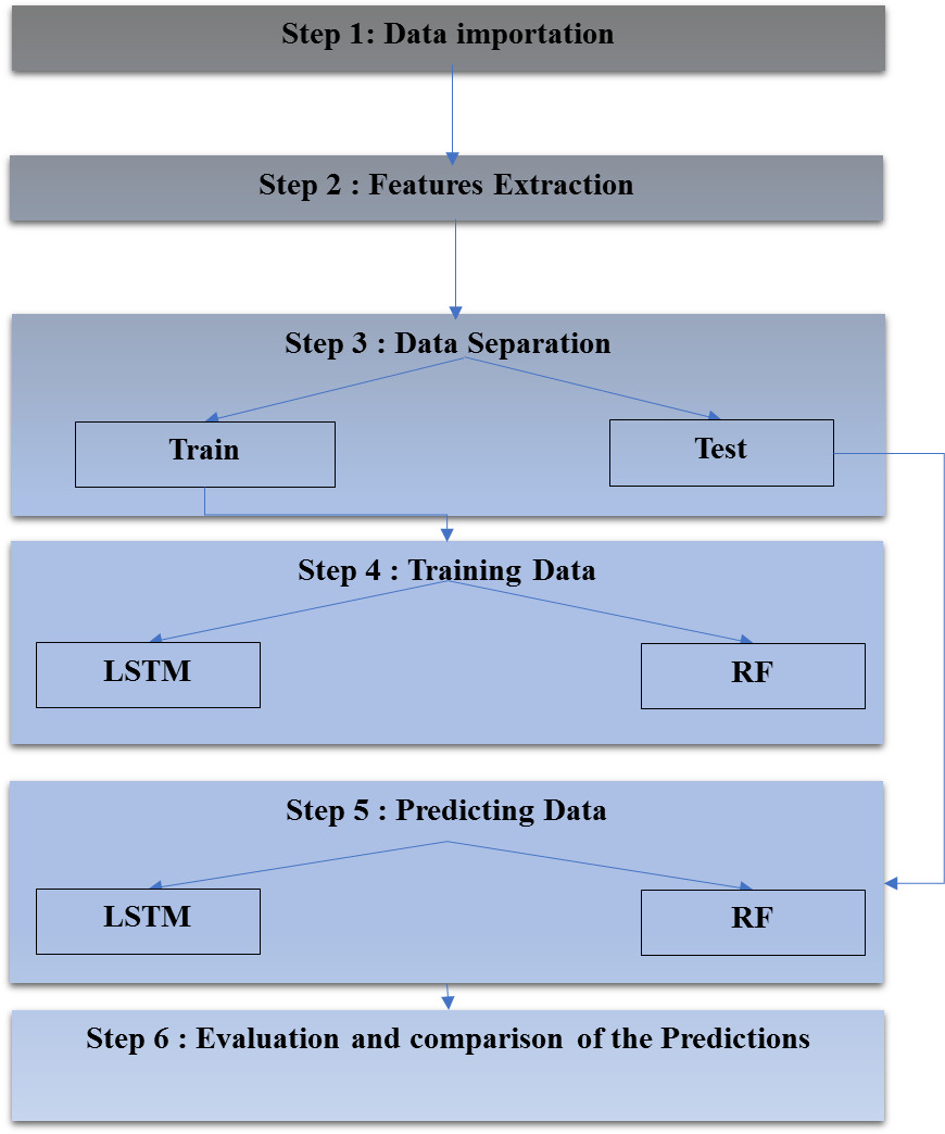
Decisions in financial markets are based on TIs to determine if the stock will increase or decrease. In this paper we will focus only on trend TIs as inputs to predict close price of stocks, the mobilised trend TIs are:
MA
The MA is one of the simplest trend indicators. It presents the evolution of the average of the previous closing prices over a given period [23]. Investors distinguish between short moving averages that vary between 5 and 50 days and long moving averages that vary between 10 and 50 weeks. Generally, investors look for short moving averages and long moving averages to cross to determine a trend. If the short moving average is above the long moving average then there is an uptrend and vice versa.
Different types of averages are distinguished, namely, Simple Moving Average (SMA), Exponential (EMA), Double Exponential (DEMA), Triple Exponential (TEMA) and Triangular (TriMA).
SMA
EMA
DEMA
TEMA
TriMA
The MACD is one of the most widely used trend indicators. This indicator is represented by three elements:
The first is the MACD line, which is the difference between the exponential moving averages of two different periods, generally 26 days and 12 days. The second is the exponential moving average of the MACD calculated over 9 days. It is called the signal line. The third is the histogram that represents the difference between the MACD and the signal line.
If the MACD is above the signal line, there is an uptrend. In the opposite case there is a downtrend [24].
“BB are evolution channels (envelope) that are plotted on either side of the MA. They are calculated by adding (upper envelope) or subtracting (lower envelope) twice the value of the standard deviation of the stock’s prices, calculated over the period of the MA. As a result, prices have a 98% chance of being within the BB” [24].
The BB were developed by John Bollinger in 1980. They are used to measure the volatility of prices. The distance of the bands from each other means that the price is volatile, and their narrowing means that the price is less volatile.
Thus, BB determine the direction of the trend. If the price oscillates between the upper band and the moving average, then the price is in an uptrend. And when it oscillates between the moving average and the lower band, then it is in a downtrend.
The ADX calculates the difference between the DMI
With DMI is the Directional Movement Index:
The SAR indicator is developed by J. Welles Wilder in 1978. This indicator is used to identify trends and potential reversal points in the market. It is calculated by determining the highest high or lowest low of a certain number of previous periods and then plotting that value on the chart. This indicator is represented by dots on the chart.
It is possible to enter a position when the price penetrates one of the SAR points:
To buy, if the price crosses above the SAR; To sell, if the price is below the SAR.
With
Mobilised features
The STDV is used to measure the dispersion or spread of a set of values around their mean. It measures the volatility in the market. If the standard deviation is high, it means that the market is volatile (risky). Conversely, it is stable [25].
Table 1 resumes the mobilised trend TIs used to train and test our models and their orders.
LSTM
The LSTM Model was developed by Hochreiter and Schmidhuber in 1997, it is an extension of the Recurrent Neural Network (RNN). This model eliminates the “Vanishing Gradient” problem encountered in RNN [8].
This problem means that the information is not preserved for a long time and the gradient becomes ineffective in the deep layers. Thus, the information of the previous instants is connected to the current instants, as long as the useful information is not too far away in time, as shown on Fig. 2.
Vanishing gradient problem.
To solve this problem, LSTM includes the “Cell State”, which is called the conveyor and acts as a memory and stores the information for deep layers. In this model each unit is linked to this conveyor, Fig. 3 illustrates the LSTM model.
LSTM schema.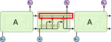
Cell state with sigmoid gates.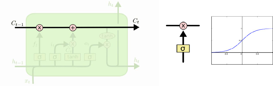
The conveyor has three bridges or “gates” that impact the transfer of information from
In the first step, “Forget gate” is used to select the information from the previous instants that should be kept or discarded with respect to the incoming training in the neuron, as shown in Fig. 5.
Forget gate.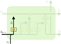
It is presented by the following function:
with, the function that provides a number between 0 and 1 depending on the importance of the information.
In the second step, it is necessary to keep the necessary information from the previous moments. The information passes through a gate
The scheme of the bridge used to keep the new information.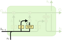
The equations associated with the gate
In the third step, we switch from the old “Cell State” to the new one. The new cell is defined as the sum of the previous retained information
The process of creating a new “Cell State”.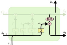
The equations associated with the creation of this new “Cell State” are the following:
In the last step, the definition of what we want to provide as output
The equations associated with this new creation are the following:
The scheme for creating the new output.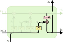
Our data is divided into 80% for training and 20% for testing. Also, for training we use MSE as a loss function, Adam optimizer and 100 epochs.
RF introduced by Breiman (2001) is a supervised ML algorithm. RF is an extension of the DT model [12].
Our RF model is based on the conventional approach given in Breiman (2001). No changes are applied to the algorithm, as we expect that the original RF may have sufficient capacity to handle a variety of variables in the datasets and result in unbiased prediction for real-world regression problems, including finance.
In essence, the RF is made of many uncorrelated deep DTs built on many data samples (Breiman, 2001). The construction process for an RF is straightforward. For every DT, we first generate a subset at random as a sample of the original data set. Next, we grow a DT with this sample to its maximum depth of
Various extensions may be made to the actual RF algorithm, like the mixed RF-neural network machine, and the multi-label learning machine advanced by RF. These approaches are interesting in that they lead to a broader diversification of the model, and can be used to increase the performance of our stock selection in the future [17].
In RF regression model, predictions are based on average predictions made by a multiple trees. In our case, we will use 100 trees, and our data are divided into 80% for train and 20% for test. Concretely, each tree of the RF is trained on a random subset of data according to the principle of bagging (correct the instability of DT by reducing the variance), with a random subset of features according to the principle of random projections (reduce the dimensionality of a set of points). The data used in RF is split into subsets, and the commonly splitting criterion used in RF is GINI index.
Results and discussion
Prediction results
Prediction results
RF architecture.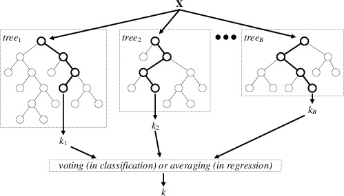
The performance evaluation of two state-of-the-art models, LSTM and RF, in predicting the behaviour of three major stocks (IAM, ATW, and BCP) is presented in the following table. The evaluation is based on three commonly used metrics in time series forecasting MSE, MAE and RMSE.
The results of this evaluation indicate that the LSTM model has a superior performance in terms of accuracy as it has a lower MSE and MAE for all three stocks. However, the RF model’s predictions are less consistent and more dispersed as demonstrated by a higher RMSE for all three stocks.
In conclusion, it is apparent that the LSTM model has a better overall performance compared to the RF model when it comes to the prediction accuracy of these stocks.
It’s worth noting that, the LSTM and RF models are both powerful tools in time series forecasting, each with their own strengths and weaknesses. However, based on the results of this specific evaluation, it appears that the LSTM model is more suitable for the prediction of these three stocks [26].
Predicting the close price of the stocks is important not only for traders but also for researchers. It helps them to take the right decisions, maximize the profit and minimize the risk if the predictions are highly accurate. But the predictions aren’t a simple task.
In this work we tried to predict the close price of three stocks listed in CSE, namely IAM, ATW and BCP. We mobilized two models and we compared their prediction performance on the daily data between 04/01/2020 and 12/11/2020. Furthermore, the input variables used in this work are only the trend TI.
As results, the LSTM is more accurate than RF and gives predictions much better. Thus, we able to state that the LSTM model is useful prediction tool for this topic and the trend TI used here proved their ability in predicting the close price, in other words this work calls into question the EMH and proves the ability to take profitability of TA.
However, the predictions of our models could be improved by adding new technical variables and using more data, and this is will be our future work. Where we are going to compare between the profitability of trend TI, oscillators and the combination between them.