
Abstract
BACKGROUND:
Like Bitcoin or any other cryptocurrencies, non-fungible tokens (NFTs) count on blockchain technology, and NFTs are the latest and the most popular in a series of blockchain solutions. Traders in this ecosystem need to pay a dynamic fee, called a gas fee, for making any transactions on the Ethereum blockchain. The gas fee is measured by gwei, and traders must consider this as an additional cost. So, the current price of this fee may affect the decision of NFT creators or traders.
OBJECTIVE:
This study investigates the interrelationships between NTFs, cryptocurrencies (Ethereum and BTC), and gas fees using daily market data from January 2019 to November 2021.
METHOD:
Fourier Shin’s (2016) cointegration test, Fully Modified Ordinary Least Squares, and Group Dynamic Least Squares tests were employed to analyze the data. Then, the variance Decomposition method was applied to determine what other variables explain the percentage of the total variance on NFTs— it also used Impulse-response functions for measuring the response of the NFTs variable for one standard deviation shock.
RESULTS:
Results show that an increase in gas fees, the daily volume of Bitcoin, and the daily volume of Ethereum decrease NFTs sales. There is a unidirectional relationship between lnSales and lnGasFee variables. Also, there is a determined unidirectional relationship between lnBTC and lnSales variables. Lastly, there is a one-way causality relationship between lnSales and lnETH variables.
CONCLUSIONS:
The primary causation of the relationship between NFTs, gas fees and Ethereum fees is most likely related to the use of Ethereum as the primary means of payment in the NFTs market and gas fees being a significant cost element in NFTs trading. Another point of view is that the dominance of Bitcoin in the market is very effective in pricing of other cryptocurrencies and in the sales and pricing of NFTs indirectly. It is supported by empirical findings that the main elements in the blockchain ecosystem are interrelated.


Introduction
Non-fungible tokens (NFTs) are the latest and the most popular in a series of blockchain solutions. NFTs have gained lots of momentum and become the new center of attention in the decentralized finance ecosystem after an NFT for a digital art by Beeple was sold at Christie’s auction house for nearly $70 million. Following the cryptocurrency market, the current popularity of NFTs are one of the most notable successes of blockchain technology [1]. Representing a radical innovation, NTFs have become a new phenomenon and attracted more users with new solutions [2]. NFTs based on innovative and unique characteristics certify ownership of digital content and assets [3] and pave the way for the digitization and trade of them [4]. These digital values can be art, videos, songs, articles, collectibles and even game objects.
Like Bitcoin or any other cryptocurrencies, NFTs rely on blockchain technology [4], and the vast majority of them are built on the Ethereum blockchain [5]. Unlike other cryptocurrencies NFTs serve as an asset representing a digital value. NFTs differ from fungible tokens such as Bitcoin or Ethereum in two major aspects. NFTs are unique and they cannot be divided or merged [6]. The interchangeability of each unit of a Bitcoin with other units of another Bitcoin makes it fungible. In other words, all Bitcoins are equivalent and indistinguishable, one Bitcoin equals any of two half Bitcoins and it is completely irrelevant which of you own. However, each NFT is unique and non-fungible. NFTs are an indivisible, irreplaceable and verifiable token that represent a digital asset [7]. The uniqueness characteristics of NFTs enable to authenticate ownership without a doubt, because there is only one token that has some specific characteristics [8].
All NFTs are tradeable in NFT marketplaces which runs in the blockchain ecosystem. Anyone to trade an NFT needs to use cryptocurrencies as a means of payment in NFT marketplace. Most of the NFT trades occur in the Ethereum blockchain which can provide smart contracts to mint NFTs. Traders need to pay a dynamic fee, called “gas fee”, for making any transactions on the Ethereum blockchain. In Ethereum blockchain, traders who pay higher fees will get an opportunity to confirm their transactions quickly [9]. The gas fee is measured by “gwei” and traders have to take this fee into account as an additional cost. Since this fee is dynamic and high particularly in Ethereum blockchain [10], the current cost of this fee may affect the decision of NFT creators or traders. Given the NFT ecosystem, we expect connectedness between NTFs and cryptocurrencies and gas fees. The main research of this paper is to investigate interconnectedness between the three of them.
The literature on NFT market is nascent and to the best of our knowledge, this is the first paper considering gas fee on NFT market and use it as a variable in econometric analysis. This paper provides novel evidence about the interrelationships between NTFs and cryptocurrencies and gas fees. The peak period of NFT’s was the third quarter of 2021 and our study contributes to NFT empirical literature covering this very recent period. To investigate the interrelationships, we use daily market data between January 2019 and November 2021. In our econometric analysis, we use Bitcoin and Ethereum volume data, representing nearly 60% of total cryptocurrency market capitalization. Bitcoin is the most dominant cryptocurrency and Ethereum is the most popular cryptocurrency used in the NFT marketplace as a means of payment. Unlike other studies, we used market volumes of Bitcoin and Ethereum instead of their prices to focus on the impact on market volume rather than pricing. We did not focus on some specific NFT markets like most of the studies and included all NFTs sale as a whole. In the analysis, we also use Gwei (gas fee), representing the cost of any transactions on the Ethereum blockchain and NFT traders have to pay.
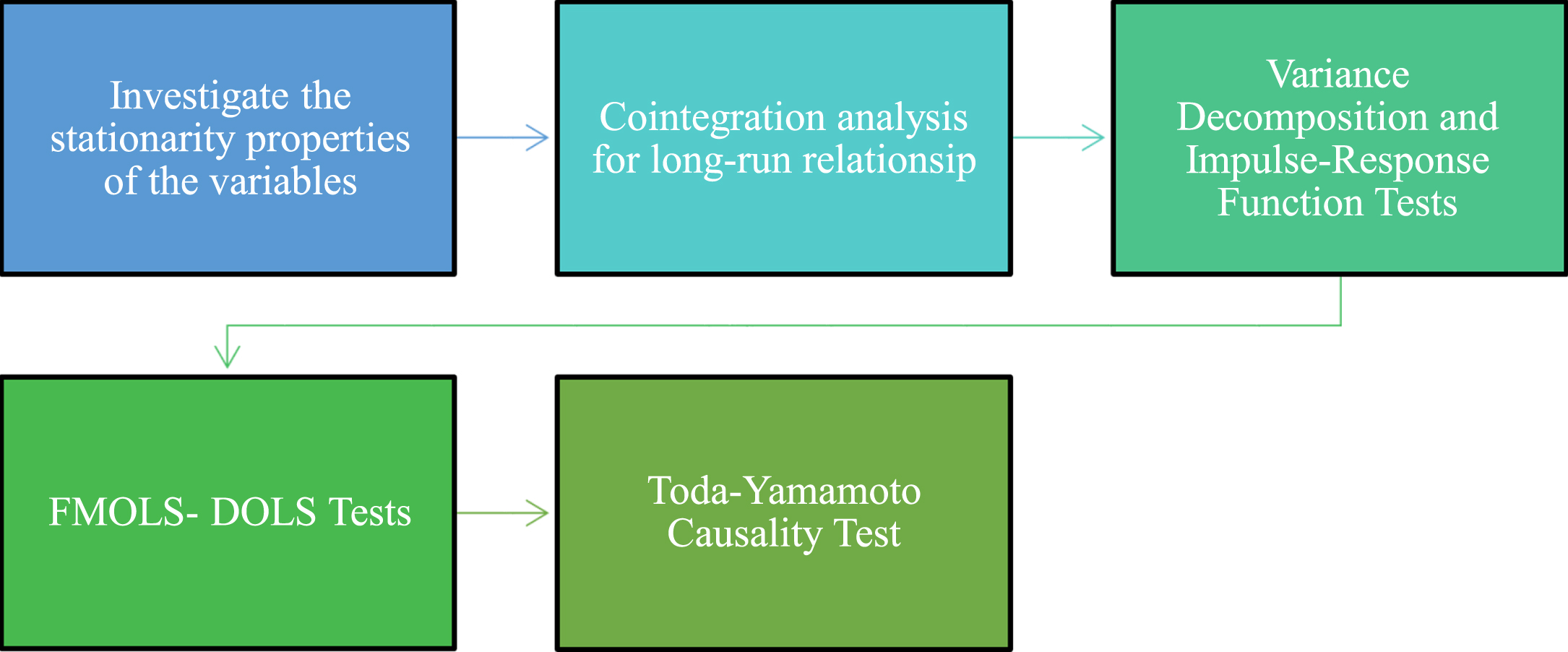
The remainder of the study addresses these neglected areas by employing more techniques to examine the hypothesized relationship between the study variables. First and foremost, the study looked into the variables’ stationarity by using the Fourier KPSS (FKPSS) Unit Root Test. After, the long-term relationship between the variables was investigated using Fourier Shin’s [11] cointegration test. Fully Modified Ordinary Least Square (FMOLS) and Dynamic Ordinary Least Square (DOLS) tests were used to interpret the coefficients of this relationship after applying the cointegration test. Then, with the variance decomposition test, the change in one of the endogenous variables was examined as separate shocks affecting all the endogenous variables. This study also explained the relationship between variables by the impulse-response test. With this test, the impact of shocks in the economic analysis of the variables used in the series was investigated. Finally, causality analysis was used in this study to determine the relationship between the variables and the direction of this relationship.
Non-fungible tokens (NFTs)
The beginning of NFT goes back to early 2010 s [12] and the first application based on NFTs using the ERC-721 was the famous virtual game CryptoKitties. The gamers spent hundreds of thousands of dollars to get ownership of cats in this virtual online game. However, the public attention towards NFTs exploded, in particular, after the Beeple’s sale in 2021, and that auction shaken up the art world. Beeples’s art named “5000 Everydays” was sold for a record 69 million USD in March 2021. That sale ranked as the most expensive NFT and the third most expensive work sold at an auction by a living artist [7]. Another prominent examples of NFTs was Twitter CEO Jack Dorsey’s tokenizing his first-ever tweet in 2006 for 2.9 million USD, and the musician RAC’s album as an NFT for 708 thousand USD [13].
The most popular NFT categories are Metaverse, Collectible, Game, Utility, DeFi, Art, Sports, and Music [10]. The NFT contents can be sold in NFT marketplaces such as OpenSea, Rarible, SuperRare, AtomicMarket, and Foundation [14]. NFT sales volume and active wallets achieved significant growth in 2021 and still increasing at a high speed as time goes. As of March 2022, the number of active wallets has reached nearly 3 million and the volume of the market has exceeded 10 billion USD (nonfungible.com). In the first quarter of 2021, sports and collectible NFTs were the most popular categories. NBA Top Shot was the platform with the highest sales volume in that quarter. Currently, a digital pet community centered around collecting, training, raising, and battling fantasy creatures called Axie ranks as the top NFT project in the first quarter of 2022 with a 3.5 billion USD all-time volume. Bored Ape Yacht Club, a collection of 10,000 Bored Ape NFTs ranks the second, CryptoPunks, 10,000 unique collectible characters with proof of ownership stored on the Ethereum blockchain ranks the third in the top NFT projects (nonfungible.com). In recent months, so-called “Metaverse”, virtual property sales setting new records [15].
In traditional marketing, it is difficult to distinguish the originals from the identical copies. However, once an NFT is recorded on the Ethereum blockchain which is supported by a digital ledger, ownership details are added to the blockchain [9]. The blockchains are transparent to all parties and provide the guarantee of nonfungibility [5]. The transparency makes all transactions, the creator, the previous and the current owner visible by everyone [7]. ERC721 is the first blockchain-based platform that has standardized the non-fungible tokens [16]. It is possible for any internet user to view even the original of the most expensive digital art, but only the person who bought the NFT tied to the art owns it [17]. There’s a big difference between seeing an art worth millions of dollars in an art museum and owning it [18]. NFTs provide legal protection to owner via the generation of third-party smart contracts [5].
The literature on NFTs is rather incipient, and focuses mostly on technical aspects [19]. Ante [20] investigates the interactions and causal relationships, short-term and long-term effects between the top 14 NFT projects. The success of the new NFT projects is influenced by that of more established markets like CryptoKitties. Another study of Ante [4] investigates the interrelations between the NFT sales and the price of Bitcoin and Ethereum. According to this study, Bitcoin price shocks trigger an increase in NFT sales, while Ethereum price shocks reduce the number of NFT wallets. This is an empirical evidence that shows the Bitcoin and Ethereum prices affect the NFT market, but not vice versa. Dowling [3] examines the pricing of NFT markets and their relationship to cryptocurrencies by using three NFT submarkets (Decentraland, CryptoPunks and Axie Infinity) markets and the prices of the two largest cryptocurrency markets (Bitcoin and Ethereum). He finds only limited volatility transmission effects between the largest cryptocurrencies and three secondary NFT market. But the wavelet coherence analysis in the paper suggests cryptocurrency pricing behavior can be helpful to understand NFT pricing patterns. Another study of Dowling [1] related to NFT pricing, examining the metaverse Decentraland parcel prices, shows that land prices characterised by inefficiency. Aharon and Demir [21] find NFTs are largely independent of shocks from other asset classes including Ethererum and most of them are attributable to endogenous shocks. Vidal-Tomas [15] analyzes short and long-term performances of NFTs focusing on metaverse and play-to-earn tokens and finds a positive performance in the long run.
Data
This study investigates the interactions between NTFs, cryptocurrencies, and gas fees. It uses the daily market data from January 2019 to November 2021. The third quarter of 2021 was the most active period for NFTs; for this reason, our data covers this most recent period. Table 1 shows the variables to be used in the analysis. Also, it demonstrates the methodology and source of these variables.
The List of Variables
The List of Variables
A longitudinal data design is used for the current study. The sales (NFT Sales) variable is used as the dependent variable, and Gas Fee, BTC (Bitcoin) and ETH (Ethereum) variables are used as independent variables with time series analyzes. This study is interested in the link between the four variables as follows:
Econometric framework.
The study follows a five-step methodological approach. Firstly, a unit root test is performed to determine the stationary levels of the variables. In the second step, long-run relationships among the variables are tested. In the third step, the effect of independent variables on the dependent variable is explained with coefficients. In the fourth step, how much the dependent variable affected itself and the independent variable in ten periods and the effect and duration of the response of the variables in ten periods are tested. In the last step, the impact of the variables on each other and the direction of this effect is revealed by a causality test.
Perron’s [22] study shows that unit root tests become less effective when structural breaks are ignored. These tests lose their validity when the fracture structure is not distinct and smoother transitions are observed [23]. In contrast to conventional unit root tests, the standard ADF unit root test is extended using Fourier functions based on a specific frequency dimension. They could obtain reliable tests regardless of time or breakage pattern by reducing the number of predicted parameters [24].
Since each time series has its characteristics, the number, duration and form of structural breaks in macroeconomic variable series vary. Enders, Becker, and Lee [25] developed the KPSS-type stationarity test by including Fourier functions in the unit root tests. Thus, it is no longer important whether the break occurs suddenly or not in determining the number of breaks by using the Fourier function [26]. The Fourier Kwiatkowski-Phillips-Schmidt-Shin test developed by [25] is independent of the break date and the number of breaks. This test allows cross-section dependence, heterogeneity, and gradual structural changes based on the Fourier stationarity test. When using trigonometric terms for nonlinear structures, this test parallels the unit root tests proposed by [27] and [28].
In the study, the equational structure of the data generation process (DGP) was created as follows:
The μt value in the equation 2-3 has an independent structure and is identically distributed with the σu2 variance. ɛt represents stationary error terms. Under the (t) approximation, the Fourier series was constructed as follows:
T and K, respectively, were indicated as the sample size and frequency values in Equations 4 [23].
The FKPSS unit root test compares the null hypothesis, “There is no unit root in the series” to the alternative, “There is a unit root in both the fixed and both fixed and trended form of the time series". The null hypothesis is not rejected if the FKPSS test statistics are lower than the critical table value determined from the simulation result [29].
After the series obtained the stationarity finding, this study examined the long-term relationship between the variables by the Fourier Shin (2016) cointegration test.
Cointegration analysis is defined as the presence of a long-term equilibrium relationship between the variables. After unit root tests determine the series’ stationarity, cointegration analysis is used to investigate the series’ relationship. Along with the cointegration test, which is the test that Engle-Granger [30] brought to the literature, new tests have emerged in the literature that also take into account structural changes. Some of these are Hatemi-J, Gregory and Hansen, and Johensen et al. The main problem seen in these tests is that the number and form of structural change are determined a priori [31].
The problems of cointegration tests were also solved by including Fourier functions in the Equation [32]. [11] and [32] have made significant progress on cointegration in their studies. For example; (11) by including the Fourier equation in the cointegration test, he was able to eliminate the lines that occur due to the number and form of structural breaks in the FKPSS test. FSHIN (cointegration) test is one of the important tests that started to be used in this way.
The Fourier SHIN (FSHIN) cointegration test was introduced to the literature by [11] and is used to test the existence, not the absence, of a long-term relationship between variables in a time series. The FSHIN cointegration test tests cointegration under the null hypothesis. [11], this test is also used as an extended version of the FKPSS stationarity test for cointegration. This test can produce strong results against structural changes such as the FKPSS test. [11] Fourier cointegration FSHIN test is expressed as follows;
In the equation is η
t
= y
t
+ v1t, y0 = 0, y
t
= yt-1 + u
t
, and x
t
= xt-1 + v2t. Here u
t
represents 0 mean
The test statistic for the FSHIN cointegration test is as follows;
The
F statistic is used in the FSHIN cointegration test and if the test statistic is smaller than the critical values of Tsong et al. (2016)’s table, it is decided that there is a cointegration relationship with structural breaks between the variables [34].
After applying the cointegration tests, FMOLS-DOLS tests were used to interpret the coefficients of this relationship. The FMOLS method was developed by [35] to obtain optimal estimates of cointegration regressions. FMOLS and DOLS methods estimate the long-term relationship in variables with the cointegration relationship. These tests can be used when the variables are I(1) or I(0). Unlike the DOLS estimator, the FMOLS method is not sensitive to the number of lag and leading values [36].
The FMOLS estimator is a semi-parametric correction method that considers the internality problem between the explanatory variables and the error term and the autocorrelation between the error terms to avoid the problems caused by the long-run correlation of the cointegrated equation and stochastic shocks [37]. FMOLS’ theoretical background is expressed as follows:
The FMOLS estimator is obtained using the following Equation (11) after calculating Equations (9) and (10):
DOLS, developed by (38) and (39), is calculated as follows:
Δ denotes the difference operator, ∂ i the coefficient of the lags and antecedents of the explanatory variables with the first difference.
The variance decomposition test examines the change in one of the endogenous variables by separating them as separate shocks affecting all the endogenous variables. In addition, variance decomposition gives information about the dynamic structure of the system. The purpose of variance decomposition is to reveal the effect of each random shock on the error variance of the prediction for future periods [40].
The dynamic behaviour of each variable in the model’s response to shocks and all other endogenous variables is described by impulse-response functions. Also, it is used to explain the relationship between variables and examine their effects on each other. Impulse-response testing investigates the impact of shocks in the economic analysis of the variables used in the series [41].
Toda-Yamamoto causality test
This study used causality analysis for determining the relationship between the variables and the direction of this relationship. Toda-Yamamoto [42] developed the Toda-Yamamoto test to investigate Granger causality tests. Based on VAR model estimation, this test takes a straightforward approach to the subject while explaining the causal relationship. This method, proposed by Toda-Yamamoto, is seen as a complementary feature of the technique he developed by [43]. This approach allows causality inferences based on an enhanced VAR model with integrated and cointegrated processes. This method is also more beneficial as it bypasses preliminary tests for unit root tests [44]. In the Toda Yamamoto causality test, which can be used if the variables become stationary due to taking both the level and the first difference, firstly, the dmax (maximum degree of integration) value calculated by the VAR method should be learned. Then, the dmax value of the variable with the highest integrated value is added to the lag length determined in the VAR model. Finally, the causality relationship is determined for the p + dmax delay value in the test [42]. The equation for the model is expressed as follows:
The k term in the equations represents the appropriate lag length. While dmax shows the maximum degree of integration, it reflects that the mean of the ɛ1t and ɛ2t error terms is zero on the equation and the covariance matrix is constant [45].
The descriptive statistics of the variables are given in Table 2.
Descriptive Statistics
Descriptive Statistics
Note: If the skewness value is < 0; skewed left, If the Skew value > 0; is skewed to the right. If the kurtosis value is < 3; engraved, if Kurtosis value > 3; it is vertical. Source: Authors.
The asymmetric distribution in the series represents the skewness value, while the Standard Deviation value states the volatility of variables for the descriptive statistic. The kurtosis coefficient value expresses the tail distribution in the series. The coefficient of variation is obtained by dividing the standard deviation by the mean. Whichever series has a higher coefficient of variation, that series shows more variability. Jarque Bera value is explained based on two main hypotheses. The first hypothesis explains the null hypothesis, which states that the series has a normal distribution. The second hypothesis expresses the alternative hypothesis that the series is not normally distributed [46]. In the study, the skewness value of the lnSales and lnGasFee variables was skewed to the right, whereas the skewness value of the lnBTC and lnETH variables was skewed to the left. The kurtosis value for lnSales and lnBTC is vertical, but it is flat for lnGasFee and lnETH. The coefficient of variation was obtained for the highest variable lnSales. Since the probability values of the Jarque Bera value are within the threshold values, it was determined that there is no normal distribution.
Table 3 shows the unit root test of the variables result. As seen in Table 3, the statistical results of the F test, which is used for the significance test of the Fourier functions of the variables, were more significant than the critical values for both the fixed and trend models. The unit root test was carried out to determine the stationarity of the variables. Determining at what level the variables are stationary is crucial for proper cointegration and other tests. The Fourier functions of the variables were significant. After these results, the null hypothesis that the series was stationary was rejected when applied FKPSS test. In other words, the smooth transitions led to the conclusion that the series contains a unit root. This study determined that the series became stationary when it took the first difference.
FKPSS Unit Root Test Results
Note: Critical values for FKPSS and F test are included in Becker et al.’s (2006) article. Source: Authors.
Cointegration tests are performed to determine a long-term relationship between variables. Table 4 presents the Fourier Shin cointegration test used to determine the relationship between equally stationary variables in the study.
Fourier Shin Cointegration Test Results
Note:
The statistical value of the F test used for the Fourier function significance test is greater than the critical values. In this case stated that Fourier function was significance.
The F test used for the Fourier function significance test had a statistical value that was higher than the critical values. In this case, it is stated that the Fourier functions are significant. As seen in Table 4, the dependent variable lnSales and all independent variables, there was a long-term relationship at the 1% significance level (lnGasFee-lnBTC-lnETH).
After applying the cointegration tests, FMOLS-DOLS tests were used to interpret the coefficients of this relationship. The FMOLS method was developed by [35] to obtain optimal estimates of cointegration regressions. FMOLS and DOLS methods estimate the long-term relationship in variables with the cointegration relationship. These tests can be used when the variables are I(1) or I(0). Unlike the DOLS estimator, the FMOLS method is not sensitive to the number of lag and leading values [36].
FMOLS and DOLS tests are used to explain how much the independent variables affect the dependent variable with coefficients. The resulting coefficients and the negative/positive nature of these coefficients explain the effect of the variables on each other and whether this effect is positive or negative. According to FMOLS and DOLS test results in Table 5, it was seen that there was a negative and long-term relationship between the variables. For FMOLS results, the lnGasFee variable had the most significant impact on lnSales. This variable was followed by lnETH (1.069) and lnBTC (0.177). According to DOLS results, lnETH (1.048) had the most significant effect on lnSales. This variable was followed by lnGasFee (0.359) and lnBTC (0.188).
FMOLS-DOLS Test Results
FMOLS-DOLS Test Results
Source: Authors.
Ten-period variance decomposition results for all variables used in the analysis were given in Table 6. This test is used to explain how many of the interactions of the variables in the ten-term process are caused by themselves and how many of them are caused by other variables. A unit change in lnSales was only due to itself in the first period. As seen in Exhibit 6, the effect of a unit change in lnSales was felt in the following periods on lnGasFee, lnBTC and lnETH variables. In the ten lagged periods, the variance of lnSales is 94% due to shocks from itself, 4.9% from lnGasFee, 0.208% from lnBTC, and 0.513% from lnETH.
Variance Decomposition Test Results (For Dependent Variable (lnSales))
Variance Decomposition Test Results (For Dependent Variable (lnSales))
Source: Authors.
The results of the Impulse-Response test graphically explain how the response of the variables in ten periods creates an effect and the duration of this effect. Used in conjunction with the Variance decomposition test, this test graphically shows how long it takes to react to shocks and variables.
As seen in Fig. 2, the reaction of lnSales to the shocks coming from itself was insignificant for the first four periods, but then the effect turned positive. While lnSales’s reaction to lnETH was meaningless in the first four periods, the effect became positive afterwards. The response of lnSales to the shocks in lnBTC and lnGasFee did not reflect a theoretical result. lnETH’s reaction to the shocks at lnSales is theoretically meaningless. InETH’s response to the shocks from him was meaningless in the first three periods, but this effect later became positive. While lnETH’s reaction to the shocks in lnBTC and lnGasFee was insignificant in the first six periods, the effect was positive afterwards.

Results of Impulse-Response Function Test.
As seen in Fig. 2, the reaction of lnBTC to the lnSales variable was economically significant and positive for the ten periods followed. While the response of lnBTC to the shocks in lnETH was inconsistent in the first five periods, this effect became positive afterwards. The reaction of lnBTC to the shocks coming from itself was economically significant and positive for the ten periods. The response of lnBTC to shocks from lnGasFee was theoretically and statistically insignificant.
The reaction of lnGasFee to the shocks in lnSales, lnBTC and lnGasFee was economically significant and positive for the ten periods followed. InGasFee’s response to the shocks from InETH did not reflect a theoretical result.
Causality analysis is used to explain the existence and direction of the relationship between variables. With the causality test, the significance level (1%, 5%, 10%) of the relationship between the variables was revealed by the analysis.
Table 7 demonstrates that at the percent 10 levels, there was a unidirectional relationship between lnSales and lnGasFee variables. Also, at the percent 5 level, was determined a unidirectional relationship between lnBTC and lnSales variables. It was determined that there is a one-way causality relationship between lnSales and lnETH variables at the 1% significance level.
Causality Test Results
Source: Authors.
Bitcoin has the highest volume in the cryptocurrency market and almost all cryptocurrencies in the market are traded with Bitcoin parity. Many of the traders in the cryptocurrency market control their capital with Bitcoin value along with USD. This dominant power of Bitcoin in the market is very effective in the pricing of other cryptocurrencies. It is an expected result that NFT trading within the blockchain ecosystem will also be affected by Bitcoin. Looking at the causality results, it is seen that NFTs (Sales) are in a one-way causality relationship with both gas fees and Ethereum. This causality is most likely related to the use of Ethereum as a main means of payment in the NFT marketplace and gas fees being a significant cost element in NFT trading. However, no causality was observed from gas fees to NFTs. This shows that NFTs sales are not affected by the increase in fees, but NFTs have an impact on fees. Similarly, there is one-way causality relationship from NFTs sales to Ethereum. While NFTs sales affect Ethereum, Ethereum volume does not affect the number of NFTs sales.
This study explored the interrelationships between NTFs, cryptocurrencies, and gas fees. The third quarter of 2021 was the highest period for NFTs, and our research adds to the empirical literature on NFTs covering this very recent period. This study used daily market data from January 2019 to November 2021 to analyze the interrelationships.
As a result of this study, the dependent variable NFT Sales and all independent variables, there was a long-term relationship at the 1% significance level. According to FMOLS and DOLS test results, it was seen that there was a negative and long-term relationship between the variables. This finding means an increase in gas fee, the daily volume of Bitcoin, and the daily volume of Ethereum decreased NFTs sales. The relationship between Ethereum, which is frequently used as a form of payment in the NFT marketplace, and the gas fee, which directly affects the cost, with NFT is a result that is consistent with the theory and natural functioning of NFT trading, which primarily occurs within the Ethereum blockchain ecosystem. Another point of view maybe is an investment substitution between NFT and cryptocurrency. Another point of view is the dominance of Bitcoin in the market is very effective in the pricing of other cryptocurrencies and indirectly in the sales and pricing of NFTs. It is supported by empirical findings that the main elements in the blockchain ecosystem as a whole are interrelated.
Furthermore, the confirmation of Bitcoin as the variable with the third-largest effect in both FMOLS and DOLS stems from Bitcoin’s dominance in the cryptocurrency market and its ability to influence the market price.
It is a fact that Bitcoin has the highest volume in the cryptocurrency market. Almost all cryptocurrencies on the market are traded in terms of Bitcoin. Most cryptocurrency investors manage their funds in terms of Bitcoin value and USD. This market dominance of Bitcoin has a significant impact on the pricing of other cryptocurrencies. Naturally, it is an expected result that NFT trading in the blockchain ecosystem will also be affected by Bitcoin. The results of the causality test also confirm this. According to the causality analysis results, it is seen that NFTs were in a one-way causality relationship with both gas fees and Ethereum fees. This causation is most likely related to the use of Ethereum as the main payment instrument in the NFT market and gas fees being a vital cost element in NFT trading. However, this study observed no causality from gas fees to NFT sales. These findings show that NFT sales are unaffected by the rise in fees, but NFTs affect fees. Similarly, there was unidirectional causality from NFT sales to Ethereum. NFT sales affect Ethereum volume, while Ethereum volume does not affect the number of NFT sales.
We expect that these findings would be useful in the decision of the NFT creators, NFT and cryptocurrency traders by presenting a statistical relationship in the blockchain ecosystem. Also, the findings would be useful for policymakers for the following and ongoing market regulation drafts and legal acts.
In future research, investigating the relationships of NFT markets with traditional investment instruments such as gold and foreign exchange or with various world stock market indices such as NASDAQ will further enrich the literature in this field. Access to short-term data is one of the limitations of this study. The effect of economic and political factors on the variables discussed in the study has been neglected, and the NFT market is a new emerging market.
Footnotes
Acknowledgments
The authors have no acknowledgments.
Author contributions
Conception: İbrahim Dağlıand Ferhat Özbay.
Methodology: Ceren Pehlivan and Ferhat Özbay.
Data collection: İbrahim Dağlı.
Interpretation or analysis of data: Ceren Pehlivan, İbrahim Dağlı, and Ferhat Özbay.
Preparation of the manuscript: Ferhat Özbay.
Revision for important intellectual content: İbrahim Dağlı, Ferhat Özbay and Ceren Pehlivan.
Supervision: İbrahim Dağlı, Ceren Pehlivan and Ferhat Özbay.