I-DLV: The new intelligent grounder of DLV

Abstract

DLV is a powerful system for Knowledge Representation and Reasoning which supports Answer Set Programming (ASP) – a logic-based programming paradigm for solving problems in a fully declarative way. DLV is currently widely used in academy, and, importantly, it has been fruitfully employed in many relevant industrial applications. Similarly to the other main-stream ASP systems, while processing an input program, in a first phase of the computation DLV eliminates the variables, thus generating a ground program which is semantically equivalent to the original one, but significantly smaller than the Herbrand Instantiation, in general. This phase, called ‘grounding’, plays a key role for the successful deployment in real-world contexts. In this work we present ℐ-DLV, a brand new version of the intelligent grounder of DLV . While relying on the solid theoretical foundations of its predecessor, it has been completely redesigned and re-engineered, both in algorithms and data structures; it now features full support to ASP-Core-2 standard language, increased flexibility and customizability, significantly improved performance, and an extensible design that eases the incorporation of language updates and optimization techniques. ℐ-DLV results in a stable and efficient ASP instantiator, that turns out to be a full-fledged deductive database system. We describe here the main features of ℐ-DLV and present the results of proper experimental activities for assessing both its applicability and performance.

Keywords

Answer Set Programming DLV Artificial Intelligence Knowledge Representation and Reasoning Grounding Instantiation Deductive Database Systems

1 Introduction

Answer Set Programming (ASP) is a purely declarative formalism, developed in the field of logic programming and nonmonotonic reasoning [7 , 48], that became widely used in AI and recognized as a powerful tool for Knowledge Representation and Reasoning (KRR). The language of ASP is based on rules, allowing (in general) for both disjunction in rule heads and nonmonotonic negation in the body; such programs are interpreted according to the answer set semantics [32, 33]. Throughout the years a significant amount of work has been carried out in order to extend the “basic” language and ease knowledge representation tasks with ASP; it has been proven to be highly versatile, offering several language constructs and reasoning modes. Moreover, the availability of reliable, high-performance implementations [11, 29] made ASP a powerful tool for developing advanced applications in many research areas, ranging from Artificial Intelligence to Databases and Bioinformatics, as well as in industrial Contexts [11 , 57].

The “traditional” approach to the evaluation of ASP programs relies on a grounding module (grounder), that generates a propositional theory semantically equivalent to the input program, coupled with a subsequent module (solver) that applies propositional techniques for generating its answer sets. There have been other attempts deviating from this customary approach [17 , 37] DBLP:conf/lpnmr/LefevreN09,lefe-nico-2009-lpnmr}; nonetheless, the majority of the current solutions relies on the canonical “ground & solve” strategy, including DLV [39] and Potassco, the Potsdam Answer Set Solving Collection [26, 27]. Among the most widely used ASP systems, DLV has been one of the first solid and reliable; its project dates back a few years after the first definition of answer set semantics [32, 33], and encompassed the development and the continuous enhancements of the system. It is widely used in academy, and, importantly, it is still employed in many relevant industrial applications, significantly contributing in spreading the use of ASP in real-world scenarios.

In this work we present ℐ-DLV, the new intelligent grounder of DLV ; starting from the solid theoretical foundations of its predecessor, it has been redesigned and re-engineered aiming at building a modern ASP instantiator marked by improved performance, native support to the ASP-Core-2 standard language [32, 33], high flexibility and customizability, and a lightweight modular design for easing the incorporation of optimization techniques and future updates. ℐ-DLV is more than an ASP grounder, resulting also in a complete and efficient deductive database system; indeed, it also keeps a set of features and capabilities that made DLV distinguishing and, especially in some industrial application domains, very popular and successful. Furthermore, ℐ-DLV is envisioned as part of a larger project aiming at a tight integration with a state-of-the-art ASP solver, a set of mechanisms and tools for interoperability and integration with other systems and formalisms, further improvements on the deductive database side, a solid base for experimenting with techniques and implementations of new approaches and applications of ASP solving, such as stream reasoning. Although the project is at the initial phase, it already shows good performance and stability, proving to be competitive both as ASP grounder and deductive database system. Furthermore, the flexible and customizable nature of ℐ-DLV allows to widely experiment with ASP and its applications and to better tailor ASP-based solutions to real-world applications. The newly herein introduced possibility of annotating ASP code with external directives to grounder is a bold move in this direction, providing a new way to fine-tune both ASP encodings and systems for any specific scenario at hand.

The present work is structured as follows. In Section 2 we introduce Answer Set Programming by first formally describing syntax and semantics, and then showing the capabilities of ASP as a KRR tool; in addition, we discuss the problem of grounding ASP programs. In Section 3 we describe the new grounder, providing the reader first with an overview of the whole computational process it is based on, and then focusing on its characteristic optimization strategies and new features; furthermore, we discuss main customization capabilities, both via command-line and by means of inline annotations. Section 4 reports the results of a thorough experimental activity that aims at assessing ℐ-DLV capabilities both as ASP grounder and deductive database system, while Section 5 discuss some related works. Eventually, in Section 6 we draw our conclusions.

2 Answer set programming

In this Section, we briefly recall syntax and semantics of ASP, and then provide, by means of proper examples, some insights about the capabilities of ASP as a tool for KRR and Deductive Databases; furthermore, we introduce the major approaches to the problem of grounding ASP programs.

A significant amount of work has been carried out by the scientific community in order to enrich the basic language of ASP, and several extensions have been studied and proposed over the years. Recently, the community agreed on a standard input language for ASP systems: ASP-Core-2, the official language of the ASP Competition series [11, 29]. We focus next on the basic aspects of the language; for a complete reference to the ASP-Core-2 standard, and further details about advanced ASP features, the reader may refer to [10] and the vast literature [4 , 47].

2.1 Syntax

A variable or a constant is a term. An atom is p (t₁, . . . , t_n), where p is a predicate of arity n and t₁, . . . , t_n are terms. A literal is either a positive literall or a negative literal not l, where l is an atom 1 . A (disjunctive) ruler has the following form:

a₁| … | a_n : -- b₁, …, b_k, not b_k+1, …, not b_m.

with n ≥ 1, m ≥ k ≥ 0, and where a₁, ⋯ , a_n, b₁, ⋯ , b_m are atoms. The disjunction a₁| ⋯ | a_n is the head of r, while the conjunction b₁, . . . , b_k, not b_k+1, . . . , not b_m is the body of r.

We denote by H (r) the set {a₁, . . . , a_n} of the head atoms, and by B (r) the set {b₁, . . . , b_k, not b_k+1, …, not b_m} of the body literals. B⁺ (r) (resp., B^- (r)) denotes the set of atoms occurring positively (resp., negatively) in B (r). For a literal L, var (L) denotes the set of variables occurring in L. For a conjunction (or a set) of literals C, var (C) denotes the set of variables occurring in the literals in C, and, for a rule r, var (r) = var (H (r)) ∪ var (B (r)). A rule having precisely one head literal (i.e. n = 1) is called a normal rule. If the body is empty (i.e. k = m = 0), it is called a fact, and we usually omit the : – sign. A rule r is safe if each variable appearing in r appears also in some positive body literal of r, i.e., var (r) = var (B⁺ (r)).

A program P is a finite set of safe rules. A term, an atom, a literal, a rule, or a program is ground if no variables appear in it.

A predicate p is referred to as an EDB predicate if, for each rule r with p ∈ H (r), r is a fact; all others predicates are referred to as IDB predicates. The set of facts in which EDB predicates occur, is called Extensional Database (EDB), the set of all other rules is the Intensional Database (IDB).

Rules without a head : –l₁, …, l_n called strong constraints, are a shorthand for false: –l₁, …, l_n. Intuitively, the body of a strong constraint must not be true in any answer set.

2.2 Semantics

Let P be a disjunctive logic program. The Herbrand universe of P, denoted as U_P, is the set of all constants appearing in P. In case no constant appears in P, an arbitrary constant ψ is added to U_P. The Herbrand base of P, denoted as B_P, is the set of all ground atoms constructible from the predicate symbols appearing in P and the constants of U_P.

Given a rule r occurring in a program P, a ground instance of r is a rule obtained from r by replacing every variable X in r by σ (X), where σ : var (r) ↦ UP is a substitution mapping the variables occurring in r to constants in UP. We denote by ground (P) the set of all the ground instances of the rules occurring in P.

An interpretation for P is a set of ground atoms, that is, an interpretation is a subset I of BP. A ground positive literal A is true (resp., false) w.r.t. I if A ∈ I (resp., A ∉ I). A ground negative literal not A is true w.r.t. I if A is false w.r.t. I; otherwise not A is false w.r.t. I.

Let r be a ground rule in ground (P). The head of r is true w.r.t. I if H (r)∩ I ≠ ∅. The body of r is true w.r.t. I if all body literals of r are true w.r.t. I (i.e., B⁺ (r) ⊆ I and B^- (r)∩ I = ∅) and is false w.r.t. I otherwise. The rule r is satisfied (or true) w.r.t. I if its head is true w.r.t. I or its body is false w.r.t. I.

A model for P is an interpretation M for P such that every rule r ∈ ground (P) is true w.r.t. M. A model M for P is minimal if no model N for P exists such that N is a proper subset of M. The set of all minimal models for P is denoted by MM (P).

Given a ground program P and an interpretation I, the reduct of P w.r.t. I is the subset P^I of P, which is obtained from P by deleting rules in which a body literal is false w.r.t. I.

Note that the above definition of reduct, proposed in [25], simplifies the original definition of Gelfond-Lifschitz (GL) transform [33], but is fully equivalent to the GL transform for the definition of answer sets [25].

Definition 1. [33, 51] Let I be an interpretation for a program P. I is an answer set for P if I ∈ MM (P^I) (i.e., I is a minimal model for the program P^I). The set of all answer sets for P is denotedby AS (P).

Example 2. Given the general logic program P₁ = { b | c : – a . , c : – not b, not a ., b | a : – not c . } and the interpretation I = {c}, the reduct P₁ ^I consists of {c : – not b, not a .}. It is easy to see that I is a minimal model of P₁ ^I , and for this reason it is also an answer set of P₁. Now, consider J = {b}. The reduct P₁ ^J is { b | a : – not c .} and it can be easily verified that J is an answer set of P₁. If, on the other hand, we take K = {a}, the reduct P₁ ^K is { b | c : – a . , b | a : – not c .} and K is not an answer set of P₁ ^K : the rule b | c : – a . , is not true w.r.t K and hence K is not a model for P₁ ^K . Indeed, it can be verified that I and J are the only answer sets of P₁.

2.3 Knowledge representation and reasoning with ASP

In the following, we briefly introduce the use of ASP as a tool for knowledge representation and reasoning, and show how its fully declarative nature allows to encode a large variety of problems via simple and elegant logic programs. It is worth noting that in an ASP program the order of rules and subgoals (literals) in rules bodies does not matter, and has no effect on the semantics; in particular, it does not affect the termination of program evaluation.

We first deal with a couple of classical deductive database applications; then, we present one of the most common ASP programming methodology, and illustrate it on a number of computationally hard problems.

2.3.1 Deductive database applications

We start illustrating an ASP-based solution to Reachability, and then deal with Same Generation.

2.3.1.1 Reachability. Given a finite directed graph G = (N, A), we want to compute all pairs of nodes (a, b) ∈ N × N such that b is reachable from a through a nonempty sequence of arcs in A. In other words, the problem amounts to computing the transitive closure of the relation A.

In the following ASP encoding, we assume that A is represented by the binary relation arc (X, Y), where a fact arc (a, b) means that G contains an arc from a to b, i.e., (a, b) ∈ A; the set of nodes N is not explicitly represented, since the nodes appearing in the transitive closure are implicitly given by these facts. Hence, the following program computes a relation reachable (X, Y) containing all facts reachable (a, b) such that b is reachable from a through the arcs of the input graph G:

reachable(X,Y) : -- arc(X,Y).

reachable(X,Y) : -- arc(X,U), reachable(U,Y).

2.3.1.2. Same generation. Given a parent-child relationship, represented by acyclic directed graph, we want to find all pairs of persons belonging to the same generation. Two persons are of the same generation if either they are siblings, or they are children of two persons of the same generation. If input is encoded by a relation parent (X, Y), where a fact parent (a, b) states that a is a parent of b, the solution can be encoded by the following program, which computes a relation samegeneration (X, Y) containing all facts such that X is of the same generationas Y:

samegeneration(X,Y)

: -- parent(P,X), parent(P,Y).

samegeneration(X,Y) : -- parent(P1,X),

parent(P2,Y), samegeneration(P1,P2).

2.3.2 The GC declarative programming methodology

We introduce here one of the most common programming paradigm in ASP, namely the Guess&Check ( GC ) Technique [19], and illustrate its application on a number of examples. Many problems can be solved in a natural manner by using this declarative programming technique: the power of disjunctive rules allows to express problems which are more complex than NP, and the (optional) separation of a fixed, non-ground program from an input database allows to do so in a uniform way over varying instances.

Given a set F_I of facts that specify an instance I of some problem P, a GC program P for P consists of the following two main parts:

Guessing Part. The guessing part G ⊆ P of the program defines the search space, such that answer sets of G ∪ F_I represent “solution candidates” for I.

Checking Part. The (optional) checking part C ⊆ P of the program filters the solution candidates in such a way that the answer sets of G ∪ C ∪ F_I represent the admissible solutions for the problem instance I.

There are no restrictions on which rules G and C may contain; hence, in the extremal case we might set G to the full program and let C be empty, i.e., checking is completely integrated into the guessing part, so that solution candidates are always solutions. Thus, both G and C may consist of arbitrary collections of rules, and it depends on the complexity of the problem at hand which kinds of rules are needed to realize these parts (in particular, the checkingpart).

The GC programming methodology has also positive implications from the “Software Engineering” point of view. Indeed, the modular program structure typical of GC allows to develop programs in an incremental fashion, which is helpful to simplify testing and debugging. For instance, one can start by writing the guessing part G and testing that G ∪ F_I correctly defines the search space, and then add the checking part and hence verify that the answer sets of G ∪ C ∪ F_I actually encode the admissible solutions.

When dealing with optimization problems, the methodology can be further extended to match a “Guess/Check/Optimize” ( GCO ) paradigm [8]: ad-hoc means for expressing preferences among answer sets are employed, such as weak constraints [8, 10], thus implementing the Optimization Part that specifies a quantitative cost evaluation of solutions. It implicitly defines an objective function f : AS (G∪ C ∪ F_I) → $ℕ$ mapping the answer sets of G ∪ C ∪ F_I to natural numbers. The semantics of G ∪ C ∪ F_I ∪ O optimizes f by filtering those answer sets featuring the minimum value; by doing so, the optimal (least cost) solutions are computed.

Let us consider a classical NP-complete problem in graph theory, namely Hamiltonian Path.

2.3.2.1. Hamiltonian path. Given a directed graph G = (N, A) and a node a ∈ N of this graph, does there exist a path in G starting from a and passing through each node in N exactly once?

If the graph G is specified by means of facts over predicates node (unary) and arc (binary), and the starting node a is specified by the predicate start (unary), then, the following GC program P_hp encodes a solution to the problem:

% Guessing Part (3 rules)

in Path(X,Y) | outPath(X,Y)

: -- start(X),arc(X,Y).

in Path(X,Y) | outPath(X,Y)

: -- reached(X),arc(X,Y).

reached(X) : -- inPath(Y,X).

% Checking Part (3 rules)

: -- inPath(X,Y),inPath(X,Y1),Y < > Y1.

: -- inPath(X,Y),inPath(X1,Y),X < > X1.

: -- node(X),not reached(X),not start(X).

In the Guessing part, the two disjunctive rules guess a subset S of the arcs to be in the path, while the rest of the program checks whether S constitutes an Hamiltonian Path. Here, an auxiliary predicate reached is used, which is associated with the guessed predicate inPath using the third rule. Note that reached is completely determined by the guess for inPath, and no further guessing is needed. In turn, through the second rule, the predicate reached influences the guess of inPath, which is made somehow inductively: initially, a guess on an arc leaving the starting node is made by the first rule, followed by repeated guesses of arcs leaving from reached nodes by the second rule, until all reached nodes have been handled.

In the Checking part, the first two constraints ensure that the set of arcs S selected by inPath meets the following requirements, which any Hamiltonian Path must satisfy: (i) there must not be two arcs starting at the same node, and (ii) there must not be two arcs ending in the same node. The third constraint enforces that all nodes in the graph are reached from the starting node in the subgraph induced by S.

It is easy to see that any set of arcs S which satisfies all three constraints must contain the arcs of a path v₀, v₁, …, v_k in G that starts at node v₀ = a, and passes through distinct nodes until no further node is left, or it arrives at the starting node a again. In the latter case, this means that the path is in fact an Hamiltonian Cycle (from which an Hamiltonian path can be immediately computed, by dropping the last arc).

Thus, given a set of facts F for node, arc, and start, the program P_hp ∪ F has an answer set if and only if the corresponding graph has an Hamiltonian Path. The above program correctly encodes the decision problem of deciding whether a given graph admits an Hamiltonian Path or not.

In the previous example we have seen how a search problem can be encoded in an ASP program whose answer sets correspond one-to-one to the solutions of the given instance. We see next another use of the GC programming technique: we build an ASP program whose answer sets witness that a property does not hold, i.e., the property at hand holds if and only if the ASP program has no answer set at all. We next apply the above programming scheme to a problem from the number and graph theories, namely Ramsey Numbers.

2.3.2.2. Ramsey numbers. The Ramsey number R (k, m) is the least integer n such that, no matter how we color the arcs of the complete undirected graph (clique) with n nodes using two colors, say red and blue, there is a red clique with k nodes (a red k-clique) or a blue clique with m nodes (a blue m-clique) [52].

We next show a program P_ramsey that allows us to decide whether a given integer n is not the Ramsey Number R (3, 4). By varying the input number n, we can determine R (3, 4), as described below. Let F be the collection of facts for input predicates node and arc encoding a complete graph with n nodes. P_ramsey is the following GC program:

% Guessing Part (1 rule)

blue(X,Y) | red(X,Y) : -- edge(X,Y).

% Checking Part (2 rules)

: -- red(X,Y), red(X,Z), red(Y,Z).

: -- blue(X,Y), blue(X,Z), blue(Y,Z),

blue(X,W), blue(Y,W), blue(Z,W).

Intuitively, the disjunctive rule guesses a color for each edge. The first constraint eliminates the colorings containing a red clique (i.e., a complete graph) with 3 nodes, and the second constraint eliminates the colorings containing a blue clique with 4 nodes. The program P_ramsey ∪ F has an answer set if and only if there is a coloring of the edges of the complete graph on n nodes containing no red clique of size 3 and no blue clique of size 4. Thus, if there is an answer set for a particular n, then n is not R (3, 4), that is, n < R (3, 4). On the other hand, if P_ramsey ∪ F has no answer set, then n ≥ R (3, 4). Thus, the smallest n such that no answer set is found is the Ramsey number R (3, 4).

2.4 Grounding for ASP computation

All currently competitive ASP systems mimic the definition of the semantics as given above by first creating a program without variables. This phase, usually referred to as instantiation or (grounding), is then followed by the answer sets search phase, in which a solver applies a propositional algorithm for finding answer sets.

The grounding solves a complex problem, which is in general EXPTIME-hard; the produced ground program is potentially of exponential size with respect to the input program [18] 2 . Grounding, hence, may be computationally expensive and has a big impact on the performance of the whole system, as its output is the input for an ASP solver, that, in the worst case, takes exponential time in the size of the input [5, 6]. Thus, given a program P, ASP grounders are geared toward efficiently producing a ground program, that is considerably smaller than Ground(P), but preserves the semantics.

The two first stable grounders have been lparse [56] and the DLV instantiator. They accept different classes of programs, and follow different strategies for the computation. The first binds non-global variables by domain predicates, to enforce ω-restrictedness [56], and instantiates a rule r scanning the extensions of the domain predicates occurring in the body of r, generating ground instances accordingly. On the other hand, the only restriction on DLV input is safety. Furthermore, the DLV instantiation strategy is based on semi-naive database techniques [58] for avoiding duplicate work, and domains are built dynamically. Over the years, a new efficient grounder has been released, namely gringo [27]. The first versions accepted only domain restricted programs with an extended notion of domain literal in order to support λ-restrictedness [30]; starting form version 3.0, gringo removed domain restrictions and instead requires programs to be safe as in DLV and evaluates them relying on semi-naive techniques as well.

3 Towards a new grounder

In this Section we introduce ℐ-DLV, the new grounder of the DLV system. As both the DLV instantiator and gringo, the core strategies rely on a bottom-up evaluation based on a semi-naive approach, which proved to be reliable and efficient over a huge number of scenarios, especially when domain extensions are very large. We discuss next the general architecture of ℐ-DLV, its typical work flow, characteristic optimization means and new features; a more thorough description of such basic techniques is available in [24].

3.1 ℐ-DLV overview

Figure 1 depicts ℐ-DLV high-level architecture. The Pre-processor module parses the input program P and builds the extensional database (EDB) from Facts(P); then, the Rewriter produces the intensional database (IDB) from the rules. The DependencyAnalyzer examines IDB rules and predicates, identifying program modules and a proper ordering for incrementally evaluating them according to the definitions in [24]. The Program Instantiator grounds the program; the process is managed by the ProgramModulesInstantiator, that, applying a semi-naive schema [24, 58], evaluates one module at a time according to the order provided by the DependencyAnalyzer. The core of the computation is performed by the RuleInstantiator: given a (non-ground) rule r and a set of ground atoms S representing predicate extensions, it generates the ground instances of r, finding proper substitutions for the variables. Notably, the set S is dynamically computed: initially, it contains only Facts(P) and from then on it is extended by the ground atoms occurring in the head of the newly generated ground rules. Ground rules are also analysed by the Simplificator, in order to check if some can be simplified or even eliminated, still guaranteeing semantics. Eventually, the output is gathered and properly arranged by the OutputBuilder. The produced ground program will have the same answer sets of the full theoretical instantiation, yet being possibly smaller [24].

Fig.1

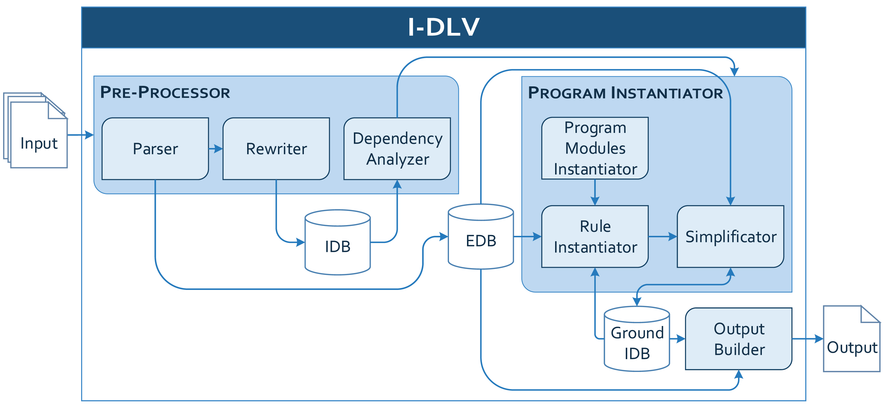
ℐ-DLV Architecture.

Thanks to the full compliance to the ASP-Core-2 standard and the capability of the OutputBuilder to format the output in different ways, including the numeric format required by state-of-the-art solvers wasp [1] and clasp [26], ℐ-DLV can be easily coupled with solvers and other ASP systems and tools.

3.2 Optimized grounding process

In the following, we better outline the computational process carried out by ℐ-DLV and discuss some of the main optimizations implemented into ℐ-DLV, pointing out the main differences with respect to the old DLV grounder. Whenever we say that some technique can be enabled/disabled on request, we imply that the grounder engine can be properly instructed by the means described in Section 3.3.

Optimizations are presented in the same order as they intervene during the grounding process, in order to help the reader at getting a general picture of the whole mechanism. Interestingly, most of them are related to different extents to the rule instantiation task, which constitutes the core of the computation and is crucial for performance; instantiating a rule basically corresponds to evaluate relational joins of the positive body literals: it requires to iterate on the literals, matching them one by one with their instances and binding the free variables accordingly, at each step. When the matching of a literal fails, backtracking to a previous literal is needed, trying to match it with another instance.

3.2.1 Managing isolated variables

At the very beginning, rules possibly undergo a rewriting process in order to remove isolated variables. For instance, consider a non-ground rule r containing a body atom p (X₁, . . . , X_n), with a variable X_i that does not appear anywhere else in r. While instantiating r, substitutions for X_i will not affect any failed match for other atoms, nor the instances obtained for the head atoms. Thus, we can safely eliminate X_i by projecting all variables X_k, k ≠ i of p to an auxiliary predicate p′. That is, a new (non-ground) rule is added: p′ (X₁, . . . , X_i-1, X_i+1, . . . , X_n) : – p (X₁, . . . , X_n) . and p (X₁, . . . , X_n) . is substituted by p′ (X₁, . . . , X_i-1, X_i+1, . . . , X_n) in the body of r. By doing so, the generation of ground instances of r which differ only on the binding of X_i is avoided. In many cases this reduces the size of the ground program, and consequently the instantiation time; nevertheless, an overhead is paid, due to the need for copying the projected instances of p in the extension of p′; such overhead, even if negligible in general, might become significant when the benefits of the projection are limited. For this reason, such projection rewriting can be disabled on request.

As a remark, the old DLV grounder was endowed with a dedicated rewriting module that implemented, among others, also this functionality. Such a module was monolithic: either all strategies were applied, or none at all. However, every rewriting shows its benefits only in specific scenarios, and can worsen performance in others; thus, the contemporary activation of many is not typically convenient.

3.2.2 Body ordering

Once the rewriting process is over, the order of literals in the rule bodies is analysed and possibly changed in a way inspired by techniques developed in the database setting, where a crucial task is to find an optimal execution ordering for the join operations. Several ordering strategies have been defined and implemented in ℐ-DLV, based on different heuristics; they perform differently, each one featuring some advantages case by case. We discuss next the Combined⁺ criterion, which is the one that better performed in the experiments, and, hence, the one that ℐ-DLV uses as default; a more thorough discussion about other criteria is out of the scope of this work. This criterion has been defined by enhancing the Combined criterion [38] already implemented in DLV . In order to highlight how the new criterion acts, we formalize first the key ideas behind the Combined criterion, and then describe its improvements.

Intuitively, given a rule r, the Combined criterion processes B (r) generating a new version of it, namely B′ (r), where the literals have been rearranged according to a greedy algorithm; at each step, the “best” literal, which is determined relying on statistics over the involved predicates, is placed, and then the statistics are updated. The “best” literal is the one that minimizes a formula (see [38]) based on two factors: one is a measure of how much the choice of a literal reduces the search space for possible substitutions, and the other takes into account the binding of the variables of the literal (indeed, preferring literals with already bound variables might lead to detecting possible inconsistencies quickly). In order to outline how the Combined⁺ criterion enhances the Combined one, we illustrate next some measures whose definition changes while moving from the old criterion to the new one.

Let us define $B_{i}^{'}$ as the reordered (partial) body at step i, and $var (B_{i}^{'})$ as the set of variables within $B_{i}^{'}$ , which is also denoted as the set of bound variables in $B_{i}^{'}$ . Given a positive literal L over a predicate p, for each variable X ∈ var (L), the selectivity of X in L (i.e. the number of distinct values), denoted V (X, L), corresponds to the number of tuples in the projection of X over the ground extension of the predicate p. Furthermore, given a rule r, for each variable X appearing in B⁺ (r), the active domain of X is defined as $dom (X) = \max_{L \in B^{+} (r)} V (X, L)$ . Being L the literal positioned at step i, i.e., $B_{i}^{'} = B_{i - 1}^{'} \cup L$ , then, for each variable $X \in var (B_{i}^{'})$ , the selectivity of X in $B_{i}^{'}$ is defined as $V (X, B_{i}^{'}) = V (X, B_{i - 1}^{'}) \cdot (V (X, L) / dom (X))$ if $X \in var (B_{i - 1}^{'})$ ; if otherwise $X \notin var (B_{i - 1}^{'})$ , then $V (X, B_{i}^{'}) = V (X, L)$ . However, according to these measures, the criterion might fail at finding a “good” ordering. As a running example, let us consider the rule: $a (X, Y, Z) : – b (X), b (Y), b (Z), Z < X, Z < Y .$

Here the criterion has no useful information for the selection of a proper order for literals b (X), b (Y), b (Z). Indeed, given that they all have the same predicate and that the considered measures do not take into account the comparisons built-in, each possible permutation of these atoms may be indiscriminately chosen.

However, their ordering can significantly affect performance, since their variables are involved in the comparisons Z < X, and Z < Y. To overcome such situations, the Combined⁺ criterion improves the cited measures relying on linear interpolation techniques to determine how much the actual search space for variables substitution is influenced by the comparisons. The new criterion preserves the assumption of uniform distribution of data already adopted in the original criterion.

Given a positive literal L over the predicate p, and a variable X ∈ var (L) which features a domain consisting of integer numbers, we define min (X, L) as the minimum value, max (X, L) as the maximum value over such domain. Please notice that the assumption over integer domains is not restrictive, as it is always possible to define a proper mapping from a generic term to a number, according to the total order of terms defined in the ASP-Core-2 standard.

Let us now describe how the Combined⁺ criterion estimates and updates the measures at each step i.

For each candidate literal L, for each variable X ∈ L, the criterion makes a pre-estimation V_e (X, B_i) of V (X, B_i) if X is an evaluable variable, that is if the following conditions hold: (i) X is not bound (i.e., $X \notin var (B_{i - 1}^{'})$ ), and (ii) X appears in B (r) in some comparisons of the form X ≺ Y, where ≺ ∈ {< , < = , > , > = , = , < >} and Y is either a ground term or a bound variable such that $Y \in var (B_{i - 1}^{'})$ .

Initially, $V_{e} (X, B_{i}^{'}) = V (X, L)$ ; then, it is recursively updated taking into account each comparison involving X and satisfying the last condition, as described next.

If X is involved in a comparison in the form X < C or X < = C where C is a ground term and C_num is the reduction of C to a numeric value, then:

$\begin{matrix} V_{e} (X, B_{i}^{'}) = & (V_{e} (X, B_{i}^{'}) - 1) \times \\ (\frac{(C_{num} - \min (X, L))}{(\max (X, L) - \min (X, L))}) . \end{matrix}$

If the comparison is of the form X > C or X > = C, then it is equivalent to C < X or C < = X, respectively; hence:

$\begin{matrix} V_{e} (X, B_{i}^{'}) = & V_{e} (X, B_{i}^{'}) - \\ ((V_{e} (X, B_{i}^{'}) - 1) \times & \frac{(C_{num} - \min (X, L))}{(\max (X, L) - \min (X, L))}) . \end{matrix}$

On the other hand, when the X is compared to a variable, such as in X ≺ Y, where ≺ ∈ {< , < = , > , > =}, then a constant value Y_num for Y is first estimated, and then the formulae above are applied; in particular, if ≺in {< , < =} then Y_num = max (Y, L₁), while if ≺in {> , > =} then Y_num = min (Y, L₁), where L₁ is the literal binding Y in B_i-1.

Finally, if X appears in a comparison in the form X = Z, where Z is either a ground term or a variable, then: $V_{e} (X, B_{i}^{'}) = \frac{1}{V_{e} (X, B_{i}^{'})}$

while if the comparison is like X ! = Z then:

$V_{e} (X, B_{i}^{'}) = V_{e} (X, B_{i}^{'}) - (\frac{1}{V_{e} (X, B_{i}^{'})}) .$

In these last two cases, indeed, the algorithm tries to estimate the probability that the value that will bound the variable X will actually be equal (or different) to the one estimated. In addition, if Z is a constant, say C, it is possible to determine with certainty if the value C is admissible or not for X, by computing if C belongs to the domain of X; otherwise, if Z is a variable, it is still possible to estimate the probability that the values assignable to Z are admissible by estimating a ground value Z_num as $1 / V (Z, B_{i - 1}^{'})$ .

After computing these pre-estimations, the criterion has a better measure of how much the comparisons can influence the variables selectivities, and thus it can properly select the next literal to add in $B_{i - 1}^{'}$ , say L′, so that $B_{i}^{'} = B_{i - 1}^{'} \cup L^{'}$ . Eventually, for each variable X ∈ L′, $V (X, B_{i}^{'})$ is updated in an unchanged way with respect to the old criterion, unless X is evaluable: in this case $V (X, B_{i}^{'}) = V_{e} (X, B_{i}^{'})$ .

Coming back to the running example, let us assume that instances for predicate b currently consists of the set b (1 . .100) (i.e., all from b (1) to b (100)); then, the Combined⁺ algorithm arranges the rule asfollows: $a (X, Y, Z) : – b (X), b (Z), Z < X, b (Y), Z < Y .$

Initially, $B_{0}^{'} = b (X)$ , and the next chosen literal is then b (Z): the algorithm prefers b (Z) over b (Y), as it computes that $V (Z, B_{1}^{'}) = 99$ and $V (Y, B_{1}^{'}) = 100$ . Intuitively, b (X) and b (Z) are here involved in a cross-product operation, thus the algorithm estimates that, in general, Z ranges over values that are smaller than the ones assigned to X in 99/100 cases, except for when they have assigned the same value. At this point, we have $B_{1}^{'} = b (X), b (Z)$ , and the comparison built-in Z < X can be safely selected: indeed, when adding a comparison literal its variables have to be bound in order to correctly evaluate them. Subsequently, b (Y), and finally Z < Y, can be chosen. It is worth noticing that an equally preferable ordering would be, in this case: $a (X, Y, Z) : – b (Y), b (Z), Z < Y, b (X), Z < X .$

Indeed, both Z < X and Z < Y have the same influence on the selectivity of Z.

3.2.3 Backjumping

Once the non-ground rules have been “adapted”, they undergo the actual rule instantiation phase, based on a backtracking search. It is worth remembering that backtracking has a great impact on the whole rule instantiation machinery: fine-tuning it might lead to great performance improvements.

ℐ-DLV employs the same non-chronological backtracking strategy of its predecessor, that reduces both the computation time and the size of the instantiation. In particular, while instantiating a rule, when a backtrack step is necessary, by considering the literal that most likely is involved in the reason of a failed match, it is possible to jump back many literals, rather than just one as in the chronological algorithm. Such “jumps” should be designed carefully, in order to avoid that some solution is missed, especially in our case, where we have to compute all (relevant) solutions. Moreover, our algorithm makes use of both semantic and structural information of the rule at hand, to compute only a relevant subset of its ground instances, yet fully preserving the semantics [50].

3.2.4 Indexing

The process is further optimized by making use of indexing techniques for the retrieval of matching instances from the predicate extensions. The indexing strategy adopted in ℐ-DLV is very flexible: any predicate argument can be indexed, allowing both single- and multiple-argument indices. For each predicate different indexing data structures can be built “on-demand”, only if needed, while instantiating a rule containing that predicate in its body.

The default configuration makes use of a heuristic which selects single- or double-indices relying on bindings; we recall here that, given a rule r whose body contains the literals L₁, …, L_n, an argument of a predicate p contained in a literal L_i is bound if it is either a ground term or contains only variables already present in some literals L_j with j = {0, …, i - 1}.

When ℐ-DLV retrieves the instances of a predicate p in r, it creates an indexing structure on-the-fly depending on its bound arguments, if needed. In particular, when multiple arguments are bound, ℐ-DLV adopts a double-argument strategy: it selects the two indexable arguments that feature the highest number of different values in the extension of p, as these are nearer to represent a double primary key for the extension of p. For instance, let us consider the rule: $a (X, Y, Z, W) : – b (X, Y), c (X, Z), d (X, Y, Z, W) .$

It is not possible to use any index for b (X, Y), due to the fact that both arguments are unbound; c (X, Z) can be indexed only on the first argument of predicate c, which is the only bound; eventually, d (X, Y, Z, W), features three bound arguments, namely the first, the second and the third, and so different indexing strategies are possible. In such situation, ℐ-DLV examines the number of different values of each bound argument, and proceeds indexing d on the most selective arguments.

An on-demand indexing strategy was present also in the old DLV grounder [15]; however, the one herein presented is more general, more flexible, and, as experiments confirmed, moreeffective.

3.2.5 Aligning substitutions

The search for an “agreement” between body literals on variable substitutions is further eased thanks to an ad-hoc mechanism that was not present in the old DLV grounder: before processing a rule r, for each variable X. Basically, we compute the intersection of all sets of possible substitutions for all the occurrences of X in r; intuitively, this reduces, in general, the number of possible values for X, by skipping those that would not match among distinct variable occurrences. Such technique performs best when the sets of substitutions differ significantly, thus can be enabled on demand.

More formally, given a predicate p of arity n, for each argument i with i ∈ {0, …, n}, ℐ-DLV stores set (p, i) as the set of possible (distinct) values for the argument i of p. Given a rule r, a variable X is said to be a “join variable” if it occurs in at least two different positive literal in B⁺ (r), and therefore if X corresponds to an argument of at least two different predicates. This alignment technique consists in determining, before the grounding of r actually starts, for each join variable X in B⁺ (r) the actual intersection of the sets set (q, j), where X is featured by the j-th arguments of the predicate q in B⁺ (r). As an example, let us consider therule r: $a (X, Y, Z) : – b (X, Y), c (Y, X, Z), d (Y, Z), e (X) .$ and in particular the variable X occurring three times in the body of r; furthermore let us suppose that |set (b, 0) |=30, |set (c, 1) |=50 and |set (e, 0) |=10. The computed intersection for X consists here in set (b, 0) ∩ set (c, 1) ∩ set (e, 0). Hence, the intersection will just contain the values on which predicates b, c and e “agree”. Intuitively, due to the presence of e (X), at most 10 values can be substituted to X in order to generate a significant substitution (i.e., a substitution that allows to obtain a relevant ground instance of r). Consequently, when substituting X with a ground value during the instantiation of r, each value that is not present in the computed intersection can be safely skipped.

3.2.6 Pushing down selections

Another optimization simulates the classic relational algebra operation of pushing selections down the execution tree. Let us consider, for instance, the following rule r: $p (X) : – t (X, Y, Z), q (Z, V, S), V < S .$

It is easy to see that, instead of first joining t with q and then selecting what complies with the comparison V < S, it is more convenient, in general, to first select, in the extension of q, the instances complying with the comparison, and then to join them with the ones of t. This can be obtained by means of a rewriting process similar to the one already described to project-out isolated variables. In order to avoid a possibly significant overhead, we do not actually perform the rewriting, but we simulate it during the instantiation of r: while retrieving the instances of q, only those complying with the comparison are actually taken into account. Such technique can be easily applied to cases in which more than one comparison occurs, and the involved terms appear in more than one atom.

This strategy, just like the one described in Section 3.2.1, was implemented in the rewriting module of DLV , whose disadvantages have already been mentioned. Furthermore, as already stated above, the technique is further optimized in ℐ-DLV, as the rewriting is performed virtually.

3.2.7 Isolated variables filtering

Just like the process of pushing down selections, the projection rewriting described above can be simulated as well during the instantiation, even if only in some cases. In particular, when instantiating a rule r, if a predicate p is solved (i.e., it is an EDB predicate, or it depends only on EDB and solved predicates), when looking for next matches for it, all instances that differ just because of the substitution of an isolated variable X could be ignored. To this end, the matching of atoms is empowered with a special filter mechanism that suggests only the relevant instances. This filter, combined with the backjumping machinery, when the projection rewriting (described in Section 3.2.1) is disabled, can simulate its behaviour without paying the overhead. However, the projection rewriting is more general, since it can safely be applied to all predicates, with no distinction between solved and unsolved; if p is unsolved, instead, all its instances must be considered as relevant in order to preserve semantics of the produced ground program; thus, the use of the described filter mechanism must be prevented.

This technique was not present in the old DLV grounder.

3.2.8 Simplifications

The output of the rule instantiation process is a set of ground instances of the rule at hand. The size of the output is further reduced by examining the produced ground rules and possibly simplifying, or even eliminating them. Indeed, body literals which are already known to be true can be safely dropped. Moreover, once the rule instance has been created, when some negative literal already known to be false occurs in the body, the rule instance is already (trivially) satisfied: it does not contribute to the semantics of the ground program, and it is removed.

In case the input program is non-disjunctive and stratified w.r.t. negation, the modular evaluation guided by the Program Modules Instantiator along with the simplification mechanism allows ℐ-DLV, just like the predecessor DLV grounder, to completely evaluate the input program: the output consists of a set of facts, that correspond to the unique answer set of the program. In such cases, there is no need to rely on a further solving module.

3.2.9 Anticipating strong constraints evaluation

The described rule grounding process can be applied also to strong constraints, with a few simplifications and adaptations due to the missing heads, when compared to “standard” rules. Notably, precisely because of this, their evaluation does not affect the aforementioned dynamic creation of the predicate extensions: thus, they could be safely processed at the very end, once the instantiation of all program modules is completed, as it was done by the old DLV grounder. However, due to the simplification mechanism, literals appearing into the body of a ground constraint can be removed, possibly leading to an empty-body constraint. By definition, such constraints are always violated; thus, the input program is inconsistent, and the grounding process can be safely aborted. For this reason, ℐ-DLV anticipates constraints grounding, and a constraint undergoes the instantiation process as soon as the extensions of its body predicates are available.

3.2.10 Magic sets

We conclude this overview with a technique for the effective use of ℐ-DLV in a deductive database setting, where efficient query answering over logic programs is essential: the magic-sets rewriting technique. It has been originally defined in [3] for non-disjunctive Datalog (i.e., with no function symbols) queries only, and afterwards many generalizations have been proposed; a thorough presentation can be found in [9, 59]. ℐ-DLV integrates an adapted version already presented in [2, 16]; in the following, we report some basic intuitions.

The magic-set method is essentially a rewriting strategy for simulating the top-down evaluation of a query: the original program is modified in order to narrow the computation to what is relevant to answer the query. Intuitively, the goal is to use the constants appearing in the query to reduce the size of the instantiation by eliminating a priori a number of ground instances of the rules which cannot contribute to the (possible) derivation of the query goal. Basically, given an input program, the binding information for IDB predicates which would be propagated during a top-down computation are materialized by means of proper adornments of the input predicates. Hence, the adorned program is used to generate a set of magic rules, which single out the atoms potentially relevant for the input query. The adorned rules are modified by adding magic atoms in the rule bodies: this limits the range of the head variables avoiding the inference of facts which cannot contribute to deriving the query. Eventually, a magic version of the query goal is produced, that will “trigger” the bottom-up generation.

The following example shows the effectiveness of the technique while dealing with the already introduced Reachability problem.

Example 3. Let us consider the program P_q-reach constituted by the encoding for the Reachability problem reported in Section 2.3.1, along with the ground query reachable (1, 5) ? and the following facts encoding a graph:

arc (1, 2) . arc (1, 3) . arc (3, 4) . arc (4, 5) . arc (2, 6) .

arc (6, 7) . arc (3, 6) . arc (7, 8) . arc (8, 6) . arc (2, 8) .

In order to answer, without the Magic Sets technique, the system should first complete the instantiation, and then check whether the query atom is actually contained in the unique answer set (we are dealing here with a stratified datalog program, hence there is no need for a solver, as discussed in Section 3.2.8). Such answer set contains 25 instances of the predicate reachable, while not all of them are (possibly) relevant in order to answer thequery.

The application of the magic-set technique would produce the following rewritten program, instead:

magic_reachable^bb(Z,Y) : -- arc(X,Z),

magic_reachable^bb(X,Y).

reachable(X,Y) : -- arc(X,Y),

magic_reachable^bb(X,Y).

reachable(X,Y) : -- magic_reachable^bb(X,Y),

arc(X,Z), reachable(Z,Y).

magic_reachable^bb(1,5).

In this rewriting, the extension of magic _reachable^bb represents the set of start- and end-nodes of all potential sub-paths of paths from 1 to 5. Therefore, when answering the query via a bottom-up computation, only these sub-paths will be actually considered: in this case, just 8 instances of magic _ reachable^bb, leading to the generation of only 3 instances of reachable.

3.3 Flexibility, customizability and further features

As already discussed, one of the main goals of the ℐ-DLV project is to obtain a novel, flexible tool for experimenting with ASP and its applications; to this end, it has been designed in order to allow a fine-grained control over the whole computational process, both via command-line options and inline annotations.

3.3.1 Command-line customization

In what follows, we describe the most relevant options that the user can set via command-line in order to customize the behaviour of ℐ-DLV. A more comprehensive list of options, along with further details, is available via the online documentation [13].

ℐ-DLV allows to completely control the indexing strategy, thus providing the user with a mean to handle situations where the default behaviour is not satisfactory. In particular, the indexing module can set per each predicate in the program a single- or multiple-index, on the desired arguments. Since only ground arguments can be indexed, if the user specifies a non indexable argument, the default indexing strategy is adopted.

As for body ordering, the user can currently choose among the following alternatives: ord₀: a basic ordering that aims at preserving the original literal positions in the rule; ord₁: the DLV Combined criterion [38]; ord₂: the aforementioned Combined⁺ criterion (enabled by default); ord₃: an enhanced version of the Combined criterion that pushes literals with functional terms down in the body; ord₄: a strategy that tries to improve the quality of available indices; ord₅: a criterion that works in synergy with backjumping in order to facilitate it; ord₆: a criterion combining the latter two.

Furthermore, the projection rewriting and the filter mechanism for isolated variables in solved predicates, both enabled by default, can be disabled. Conversely, the technique to align variable substitutions can be enabled at will: it is disabled by default, given that its benefits strictly depend from the distribution of the input data.

By default, choice rules are natively managed by directly instantiating them, possibly undergoing a conservative rewriting/rearrangement that aims at optimizing efficiency; however, the user can ask for a rewriting approach that makes use of disjunction and removes them, thus generating a choice-rule-free program. Both approaches preserve thesemantics.

ℐ-DLV is able to process both ground and non-ground queries. By default, it simply produces the instantiation; upon request, for non-disjunctive and stratified programs, that are completely evaluated by the system, it can directly provide the query answer. The magic-set technique, enabled by default, can be disabled.

For advanced users, insights on the grounding process might be of great interest: they are available via a number of statistics that can be produced on demand. In particular, the following information are provided for each input rule: total instantiation time, number of produced ground instances, number of iterations required for instantiation (in case the rule is recursive); in addition, size of extension and selectivity of all arguments are reported, for each predicate in the rule.

3.3.2 Inline customization and optimizations via annotations

In order to ease and improve system customization and tuning, ℐ-DLV introduces a new special feature: annotations of ASP code.

Annotations and meta-data have been applied in different programming paradigms and languages; Java annotations, for instance, have no direct effect on the code they annotate: a typical usage consists in analysing them at runtime in order to change the code behaviour. Some sorts of annotations have been proposed also for declarative paradigms, although to different extents and purposes with respect to our setting; a more detailed discussion is carried out in Section 5.

ℐ-DLV annotations allow to give explicit directions on the internal grounding process, at a more fine-grained level with respect to the command-line options: they “annotate” the ASP code in a Java-like fashion, while embedded in comments: hence, the resulting programs can still be given as input to other ASP systems that do not support them, without any modification. In particular, our annotations can have two different scopes: at the global level, meaning that they are applied to the whole program, or at the rule level, and hence annotations acts just on the rule they precede.

Syntactically, all annotations start with the prefix “% @” and end with a dot (“.”). The current ℐ-DLV release supports annotations for customizing two of the major aspects of the grounding process: body ordering and indexing; additional options are being developed.

A specific body ordering strategy can be explicitly requested for any rule, simply preceding it with the line:

% @rule_ordering(@value=Ordering_Type).

where Ordering_Type is a number representing an ordering strategy (Section 3.3.1). In addition, it is possible to specify a particular partial order among atoms, no matter the employed ordering strategy, by means of before and after directives. For instance, in the next example, ℐ-DLV is forced to always put literals a (X, Y) and X = # count {Z : c (Z)}} before literal f (X, Y), whatever the order chosen:

% @rule_partial_order(

@before={a(X,Y), X=#count{Z:c(Z)}},

@after={f(X,Y)}).

As for indexing, directives on a per-atom basis can be given; the next annotation, for instance, requests that, in the subsequent rule, atom a (X, Y, Z) is indexed, if possible, with a double-index on the first and third arguments:

% @rule_atom_indexed(@atom=a(X,Y,Z),

@arguments={0,2}).

Multiple preferences can be expressed via different annotations; in case of conflicts, priority is given to the first appearing in the program. In addition, preferences can also be specified at a global scope, by replacing the rule directive with the global one. Such kind of annotations are applied on the rules, if possible. While a rule annotation must precede the intended rule, global annotations can appear at any line in the input program. Both global and rule annotations can be expressed in the same program; in case of overlap on a particular rule/setting, priority is given to the more specific rule ones.

Intuitively, the way annotations change the grounding mechanisms can noticeably affect performance on the program at hand; in order to give an idea, we illustrate next a few interesting cases related to problems featured in the 6th ASP Competition benchmark suite (see Section 4), where performance is significantly affected by the body orderings. It is worth noting that the heuristic-based nature of the default ordering criterion (see Section 3.2.2) does not guarantee optimality, and thus it is possible that the introduction of further policies, directly indicated by the user or inferred from other criteria, lead to a better-performing ordering. Indeed, in the following examples the standard strategy turns out as not the best one: customization via annotations allows the grounder to improve efficiency. As first example let us consider the rule:

reach (X, Y, T) : –reach (XX, YY, T) ,

dneighbor (D, XX, YY, X, Y) ,

conn (XX, YY, D, T) , conn (X, Y, E, T) ,

inverse (D, E) , step (T) .

which is taken from the encoding of Labyrinth. In this case, by annotating the rule with:

% @rule_partial_order(

@before={inverse(D,E)},

@after={reach(XX,YY,T),

dneighbor(D,XX,YY,X,Y),

conn(XX,YY,D,T), conn(X,Y,E,T),

step(T).}).

that corresponds to ask ℐ-DLV to select as first literals inverse (D, E) in its ordering strategy no matter how the other literals are positioned, average grounding time over all instances is reduced up to 90%. Similarly, by annotating the following rule in the Visit-all encoding:

% @rule_ordering(@value=5).

atother (N, T) : – connected (C, N) , C ! = N,

step (T) , atrobot (O, T) , O ! = N .

that requires the use of criterion ord₅ instead of the default one on this specific rule, the average grounding time computed over all instances reduces by 15%; the same improvement is obtained with the ordering criterion ord₆. Having a closer look at what changes, we can observe that while the default algorithm orders the rule body as already reported, the mentioned criteria orders the body as follows:

atother (N, T) : – atrobot (O, T) , step (T) ,

connected (C, N) , C ! = N, O ! = N .

Let us give some insights about the reasons of the performance improvements. In the case of Labyrinth instances, intuitively, since the extension of the predicate inverse is very small, it is better to add it as soon as possible, possibly at first. As for Visit-all, both criteria ord₅ and ord₆ try to prefer literals binding output variables (i.e., variables appearing in head or in body literals with unsolved predicates) in order to facilitate the backjumping mechanism. In that rule, the output variables are N, T and O, and thus the literal atrobot (O, T) is inserted as soon as possible (in fact, it is the one containing the largest number of output variables).

It is worth noting that, in all reported cases, acting at a global scope, as one could do via command-line options, does not bring the same improvements: indeed, experiments showed that the gain due to the change of strategy over the reported rules is overshadowed by corresponding losses over the rest of the program; the flexible customization means featured by ℐ-DLV, that allows to configure and fine-tune the grounder as needed, even at a rule level, are exactly aimed at better dealing with such scenarios.

4 Experimental evaluation

Hereafter we report the results of an experimental activity carried out to assess ℐ-DLV performance as both ASP grounder and deductive database system. In order to obtain trustworthy results, we considered tests that have already been largely used and are publicly available. In particular, we relied on:

the whole 6th ASP Competition suite [28], the latest edition of a series of events [11, 29] assessing ASP systems on challenging benchmarks, in order to promote state of the art techniques and language standards;

OpenRuleBench [42], an open (freely available) set of resources comprising a suite of benchmarks for analysing performance and scalability of different rule engines;

a suite of benchmarks employed in literature to test Consistent Query Answering (CQA) systems on large inconsistent database [34, 35].

Experiments have been performed on a NUMA machine equipped with two 2.8GHz AMD Opteron6320 processors and 128 GiB of main memory, running Linux Ubuntu14.04.4(kernel v.3.19.0-25). Binaries were generated with the GNU C++compilerv. 4.8.4. As for memory and time limits, we allotted 15 GiB and 600 seconds for each system, per each single run.

4.1. ASP grounding benchmarks. For this setting we tested ℐ-DLV against the two mainstream grounders gringo and the (old) intelligent grounder of DLV , and in particular the latest available versions at the time of writing: 4.5.4 and 2012-12-17, respectively. We first launched the 6th ASP Competition suite, that features 28 problems and 20 different instances per each. Results are reported in Fig. 2: first column shows the name of the problem, while the next three report the average times. Dashes in the column of a system means that it has not been tested on the corresponding problem: this was due, for gringo, to the presence of queries in three cases, and for DLV to the missing support for relevant ASP-Core-2 constructs. When launched, all systems were able to ground all 20 instances in the allotted time. It is evident, while comparing ℐ-DLV against DLV , that the new grounder systematically outperforms its predecessor, enjoying performance gains up to 90%. Also the comparison with gringo is encouraging: despite the prototypical version of ℐ-DLV, it proves to be competitive. More in detail, excluding the 3 domains solved only by ℐ-DLV, times are substantially aligned (time differences below 20%) in 9 domains out of 25; as for the remaining domains, each outperforms the other in an almost equal number of domains.

Fig.2

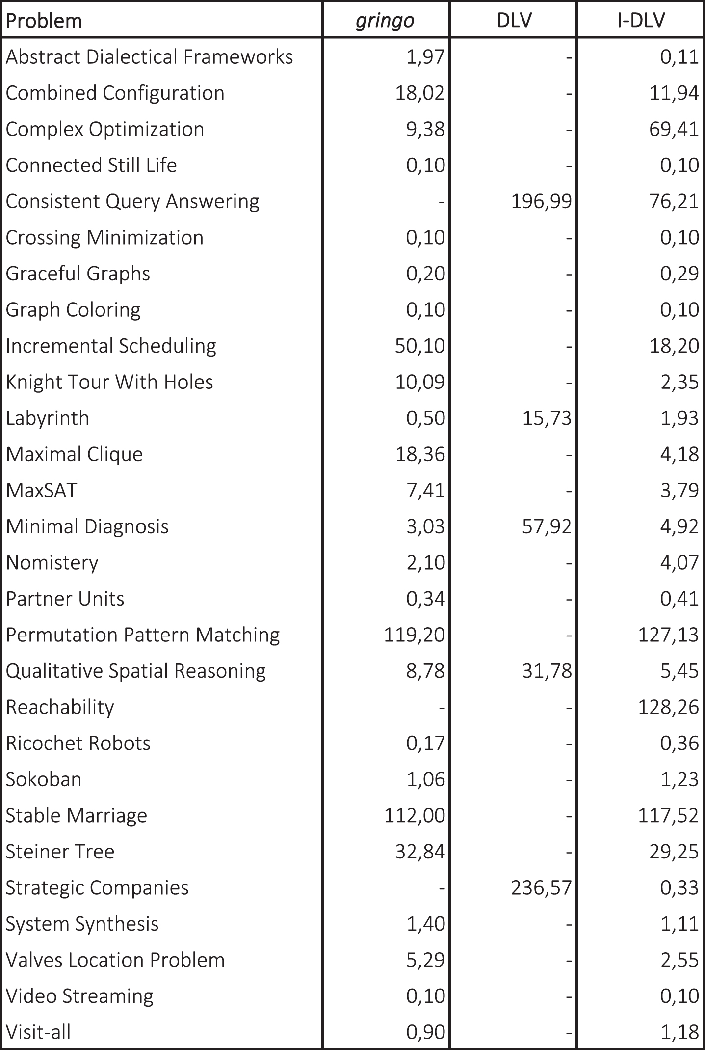
Benchmarks from 6th ASP Competition – grounding times in seconds.

In order to find further comparison settings outside of the ASP Competition series, where gringo became the de facto standard grounder for all competing solvers, we took into account the problems appearing in OpenRuleBench and in CQA benchmarks. This is also motivated by the fact that the ASP Competition mainly focuses on problems where solving task is more relevant with respect to the grounding one (indeed, as Fig. 2 shows, all systems completed all instances), while OpenRuleBench and the selected tests from CQA suite demand a more significant work from the grounders.

Regarding OpenRuleBench, since it consists essentially of a query-based set of problems, that gringo would not accept “as-is”, we removed the query from the encodings and measured just the grounding times. Obviously, we did the same also for the DLV instantiator and ℐ-DLV: otherwise, these might have taken advantage from the magic-set technique, thus leading to an unfair test. Results are reported in Fig. 3: after domains names and corresponding number of instances, the next three pairs of columns show the number of solved instances and the running time averaged over solved instances. Last line reports the total running times for each system (600 secs is added for unsolved instances, as systems were stopped if unable to finish before). The unique dash in the table corresponds to a domain for which DLV did not solve any instance within the allotted time. Interestingly, even if DLV is outperformed by both gringo and ℐ-DLV, its performance are somehow satisfactory, still confirming its solidity and reliability. As for gringo and ℐ-DLV, both solved 101 instances out of 108; however, ℐ-DLV appears to enjoy better performance: it clearly outperforms gringo in almost all domains.

Fig.3

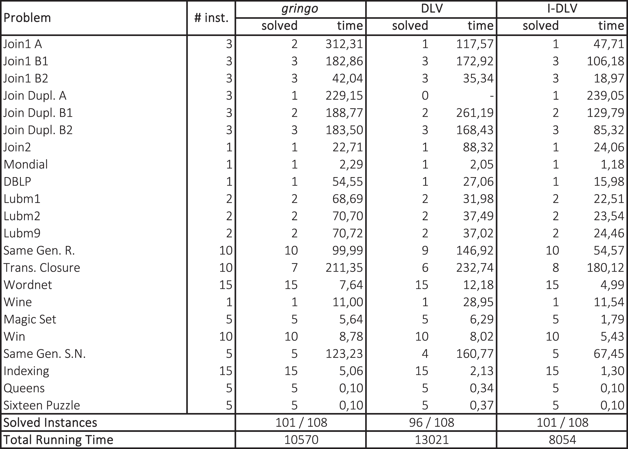
OpenRuleBench Benchmarks – grounding times in seconds.

As for the CQA benchmarks, we selected a single database among the four available: indeed, they are randomly generated, and from a grounding perspective performance was very similar; moreover, among the available encoding we chose the Pruning one introduced in [45], as it was shown to be the one on which most of the execution time is spent on grounding. The executed part of the benchmark consists in 10 instances with increasing sizes, varying from 100k to 1M tuples, and 21 encodings obtained by combining the Pruning encoding with 21 different extensions each one simulating a different database query. It is worth noticing that, in order to fairly test DLV and ℐ-DLV against gringo, no encoding contains a query explicitly expressed in ASP: queries are simulated via plain normal rules. Figure 4 shows the average grounding times for each encoding on the 10 instances: gringo and ℐ-DLV were able to ground the whole suite within the given limits, while DLV was not able to execute any problem due to the presence of choice rules, which are not supported by the system. Also in this case, the results confirm the reliability of ℐ-DLV, which obtained the best performance on each problem, even if the special optimization means for query answering could not be employed due to the lack of explicitly expressed queries.

Fig.4

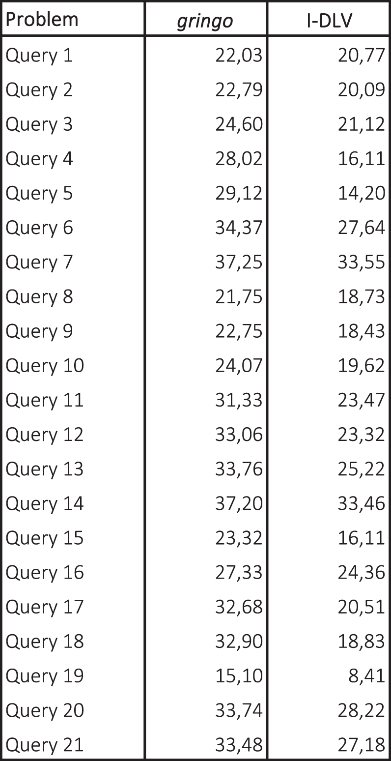
CQA Benchmarks – grounding times in seconds.

4.2. Deductive database benchmarks. For this setting, the natural choice was the query-based set of problems of the OpenRuleBench initiative. Besides DLV , we tested ℐ-DLV against XSB [55] (the latest available version, 3.6) which was among the clear winners and is currently one of the most widespread Logic Programming and Deductive Database systems. All systems support query answering, thus, differently from above, queries have not been removed. Results are reported in Fig. 5: after domain names and corresponding number of instances, the next three pairs of columns show the number of solved instances and the running time averaged over solved instances. Similarly as above, last line reports the total running times for each system. The unique dash in the table corresponds to a domain for which DLV did not solve any instance within the allotted time. Also in this setting, results are very encouraging: not only ℐ-DLV behaves better than DLV , but it is definitely competitive against XSB. Indeed, in spite of a non-negligible variability from a problem to another, ℐ-DLV times are, on the overall, comparable with the ones of XSB; in addition, it was able to solve even more instances within the allotted time (123 for ℐ-DLV, 115 for XSB). Interestingly, XSB has been launched with the exact OpenRuleBench settings, where the best configuration was set manually per each problem; ℐ-DLV, instead, features the same default configuration over all domains. As already stated, a thorough study of the impact on performance due to ℐ-DLV fine-tuning capabilities is out of the scope of the present work; an analysis of possible performance improvements due to a specific customization on each single problem in this setting will be definitely of interest.

Fig.5

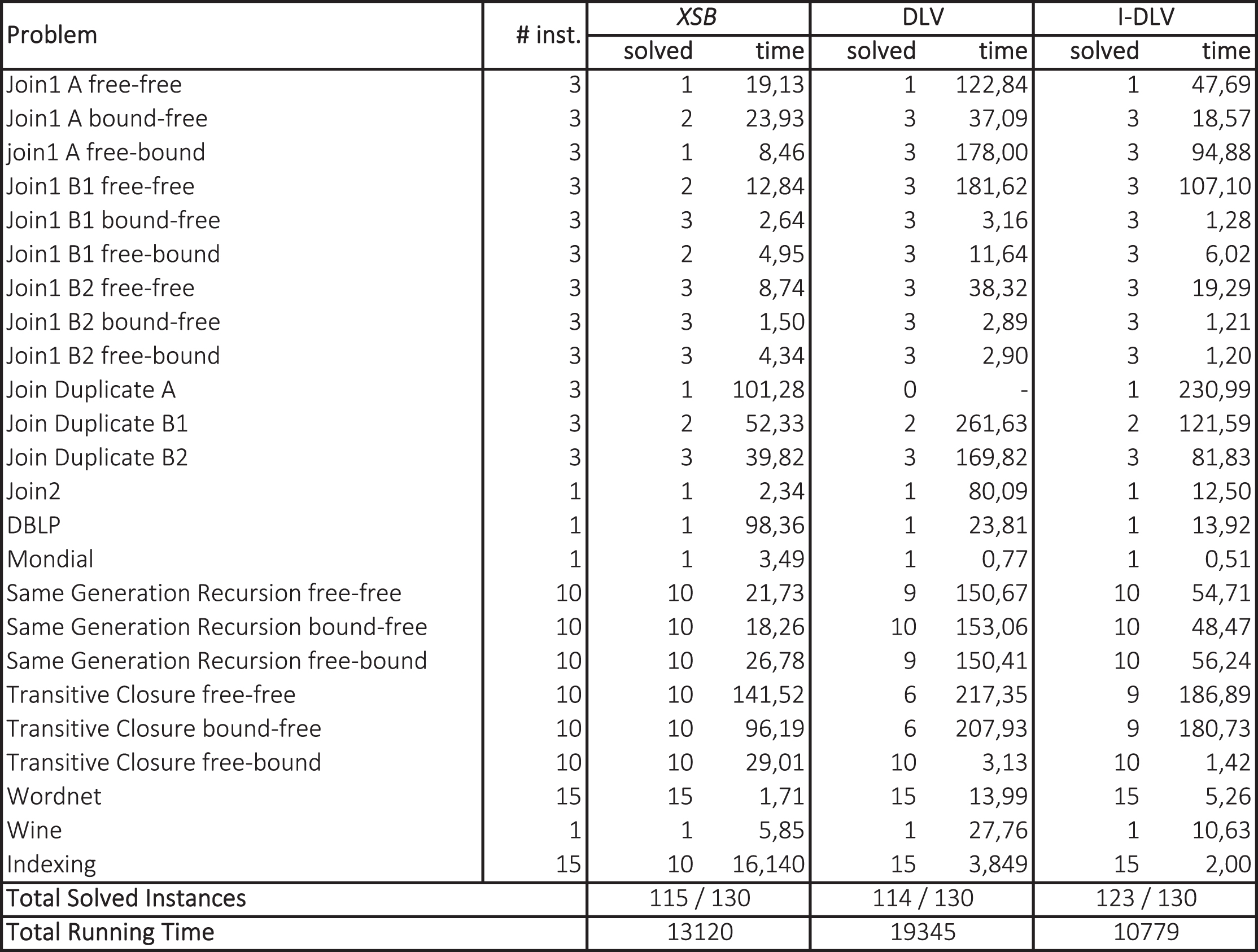
Benchmarks from OpenRuleBench – query answering times in seconds.

5 Related works

Some connections to our work can be found with other rule-based engines and deductive database systems; an interesting overview can be found in [43]. Such systems have common roots, even though differ in several aspects, especially with respect to supported languages and evaluation mechanisms; in particular, XSB [55], among the most prominent, is indeed a Prolog system which relies on a top-down evaluation. ℐ-DLV as already discussed in this work, is an ASP grounder relying on a bottom-upapproach.

As for grounding processes, different approaches are pursued by lparse [56], that supports ω-restricted [56] programs, and GidL [62], a grounder for FO⁺. Nevertheless, stronger connections can be found with the other state-of-the-art ASP grounders, such as the grounder module of DLV [24], and gringo [27]: they all share the basic evaluation approach.

Although stemming from common roots with the DLV grounder, ℐ-DLV features many differences and novelties. From the syntactic point of view, contrarily from its predecessor, ℐ-DLV fully supports the ASP-Core-2 standard language, and hence it can interoperate with the state-of-the-art solver modules. It maintains a similar backjumping mechanism to process rule instantiation along with the magic sets technique for query answering, and incorporates improved optimizations that impact over all phases of the computational machinery, such as body ordering and indexing. Moreover, ℐ-DLV introduces many new optimization means that guarantee better performance (see Section 4).

The grounder gringo constituted, so far, the only ASP grounder supporting the ASP-Core-2 standard and hence able to interoperate with solvers, thus becoming the most commonly used ASP grounder, as emerged from the last ASP Competitions; it is also a long-lasting player, part of a larger family of Answer Set Programming tools that already optimize interoperation. Similarly to gringo, in order to improve performance, ℐ-DLV incorporates different optimization techniques; yet, it features novel customization properties, such annotations and special command-line options. Furthermore, differently from gringo, ℐ-DLV implements specific deductive-database-oriented features, such as Magic Sets: when answering a query, these allow to avoid the grounding of the whole input program, just requiring the grounding of a selected (and ad-hoc rewritten) part of it.

The usage of annotations has already been proposed in the literature [35 , 61]. The work In [61] is one of the most related to our setting, as applies annotations to ASP programs. In particular, it introduces the language LANA, that allows one to express meta-information that acts as an external tool for development support (such as documentation, testing, verification, or code completion); therefore, annotations do not have a direct impact on program evaluation. Similarly, the work in [35] refers to annotations as a tool for better documenting Prolog programs, while the one in [53] is oriented towards semantic annotations of ontologies. A different approach is pursued in [20], where some syntactic means for expressing (desirable) properties of ASP HEX programs are introduced. However, the aim of the introduction of annotations in ℐ-DLV is different from the mentioned mechanisms: as described in Section 3, they allow an inline customization of the actual grounding machinery: it acts internally, by changing the behaviour of the system that can hence be “trained ” in order to follow specific user’s desiderata related to the groundingprocess.

6 Conclusions

In this work we introduced ℐ-DLV, the new grounder of the DLV system. With respect to its predecessor, it features full support to the ASP-Core-2 standard, new optimization techniques, new features and customization capabilities, as well as interoperability with current state-of-the-art ASP Solvers and improved performance.

Besides experiments and further optimizations, ongoing work focuses on studying and experimenting with a tight integration with a state-of-the art ASP solver, equipping it with a set of advanced mechanisms and tools for interoperability and integration with other systems and formalisms, and enriching it with additional database-oriented functionalities. Moreover, we plan to properly experiment with the customization capabilities of the system, further extending them, for instance by widening the range of aspects over which annotations canintervene.

ℐ-DLV source and binaries are available from the official repository [14].

Footnotes

Without loss of generality, in this paper we do not consider strong negation, which is irrelevant for the instantiation process; the symbol ‘not ’ denotes default negation here.

Hence, producing the ground instantiation may require an exponential time in the size of the input program. In order to grasp the intuition consider the following program containing only one non-ground rule: obj (0) . obj (1) . disp (X₁, …, X_n) : – obj (X₁) , …, obj (X_n) . It is easy to see that the corresponding ground instantiation contains 2ⁿ + 2 rules. For more details about complexity results the reader may refer to [18 , ].

References

Alviano

, Dodaro

, Leone

and Ricca

, Advances in WASP. In Calimeri et al. [12], pp. 40–54.

Alviano

, Faber

, Greco

and Leone

, Magic sets for disjunctive datalog programs. Artificial Intelligence187 (2012), 156–192.

Bancilhon

, Maier

, Sagiv

and Ullman

J.D.

, Magic Sets and Other Strange Ways to Implement Logic Programs, In Proceedings of the Fifth ACM SIGACT-SIGMOD Symposium on Principles of Database Systems, Cambridge, Massachusetts, 1986, pp. 1–15 .

Baral

, Knowledge Representation, Reasoning and Declarative Problem Solving, Cambridge University Press, 2003.

Ben-Eliyahu

and Dechter

, Propositional semantics for disjunctive logic programs. Annals of Mathematics and Artificial Intelligence12 (1994), 53–87.

Ben-Eliyahu

and Palopoli.

, Reasoning with Minimal Models: Efficient Algorithms and Applications. In Proceedings Fourth International Conference on Principles of Knowledge Representation and Reasoning (KR-94) (1994), 39–50.

Brewka

, Eiter

and Truszczynski

, Answer set programming at a glance. Communications of the ACM54(12) (2011), 92–103.

Buccafurri

, Leone

and Rullo.

, Strong and Weak Constraints in Disjunctive Datalog. In Dix

Jürgen

, Furbach

Ulrich

, and Nerode

Anil

, editors, Proceedings of the 4th International Conference on Logic Programming and Non-Monotonic Reasoning (LPNMR’97), volume 1265of Lecture Notes in AI (LNAI), Dagstuhl, Germany, 1997, pp. 2–17. Springer Verlag.

Calimeri

, Cozza

, Ianni

and Leone

, Magic sets for the bottom-up evaluation of finitely recursive programs. In Erdem et al. [23], pp. 71–86.

10.

Calimeri

, Faber

, Gebser

, Ianni

, Kaminski

, Krennwallner

, Leone

, Ricca

and Schaub

, Asp-core-2: Input language format, 2012. https://www.mat.unical.it/aspcomp2013/files/ASP-CORE-2.03b.pdf

11.

Calimeri

, Gebser

, Maratea

and Ricca

, Design and results of the fifth answer set programming competition. Artificial Intelligence231 (2016), 151–181.

12.

Calimeri

, Ianni

, Truszczynski

, and editors., Logic Programming and Nonmonotonic Reasoning - 13th International Conference, LPNMR 2015, Lexington, KY, USA, September 27-30, 2015. Proceedings, volume 9345of LNCS. Springer, 2015

13.

Calimeri

, Perri

, Fuscá

and Zangari

, I-DLV homepage, since 2016. https://github.com/DeMaCS-UNICAL/I-DLV/wiki

14.

Calimeri

, Perri

, Fuscá

and Zangari

, I-DLV repository, since 2016. https://github.com/DeMaCS-UNICAL/I-DLV

15.

Catalano

, Leone

and Perri

, On demand indexing techniques for the dlv instantiator. In Proceedings of the Workshop on Answer Set Programming and Other Computing Paradigms (ASPOCP 2008), Udine, Italy, 2008.

16.

Cumbo

, Faber

, Greco

and Leone

, Enhancing the magic-set method for disjunctive datalog programs. In Proceedings of the the 20th International Conference on Logic Programming – ICLP’04 volume 3132of Lecture Notes in Computer Science, 2004, 371–385.

17.

Dal Palú

, Dovier

, Pontelli

and Rossi

, GASP: Answer set programming with lazy grounding. Fundamenta Informaticae96(3) (2009), 297–322.

18.

Dantsin

, Eiter

, Gottlob

and Voronkov

, Complexity and Expressive Power of Logic Programming. ACM Computing Surveys33(3) (2001), 374–425.

19.

Eiter

, Faber

, Leone

and Pfeifer

, Declarative problem-solving using the DLV system. In Logic-based artificial intelligence, Springer, 2000, pp. 79–103.

20.

Eiter

, Fink

, Krennwallner

and Redl

, Liberal safety for answer set programs with external sources. In desJardins

Marie

and Littman

Michael L.

, editors, July 14-18, 2013, Bellevue, Washington, USA. AAAI Press, 2013.

21.

Eiter

, Gottlob

and Mannila

, Disjunctive Datalog. ACM Transactions on Database Systems22(3) (1997), 364–418.

22.

Eiter

, Ianni

and Krennwallner

, Answer Set Programming: A Primer. In Reasoning Web. Semantic Technologies for Information Systems. 5th International Summer School - Tutorial Lectures, Brixen-Bressanone, Italy, 2009, pp. 40–110.

23.

Erdem

, Lin

, Schaub

and editors, Logic Programming and Nonmonotonic Reasoning, 10th International Conference, LPNMR 2009, Potsdam, Germany, September 14-18, 2009. Proceedings, volume 5753of Lecture Notes in Computer Science. Springer, 2009.

24.

Faber

, Leone

and Perri

, The intelligent grounder of DLV. In Erdem

Esra

, Lee

Joohyung

, Lierler

Yuliya

, and Pearce

David

, editors, Correct Reasoning - Essays on Logic-Based AI in Honour of Vladimir Lifschitz, volume 7265of LNCS, Springer, 2012, pp. 247–264.

25.

Faber

, Leone

and Pfeifer

, Recursive aggregates in disjunctive logic programs: Semantics and complexity. In Alferes

José Júlio

and Leite

João

, editors, Proceedings of the 9th European Conference on Artificial Intelligence (JELIA 2004), volume 3229of Lecture Notes in AI (LNAI), Springer Verlag, September2004, pp. 200–212.

26.

Gebser

, Kaminski

, Kaufmann

, Romero

and Schaub

, Progress in clasp series 3. In Calimeri et al. [12], pp. 368–383.

27.

Gebser

, Kaminski

, König

and Schaub

, Advances in gringo series 3. In Logic Programming and Nonmonotonic Reasoning - 11th International Conference, LPNMR 2011, Vancouver, Canada, May 16-19, 2011. Proceedings, volume 6645of Lecture Notes in Computer Science, Springer, 2011, pp. 345–351.

28.

Gebser

, Maratea

and Ricca

, The Design of the Sixth Answer Set Programming Competition. In Calimeri et al. [12] pp. 531–544.

29.

Gebser

, Maratea

and Ricca

, What’s hot in the answer set programming competition. In Schuurmans

Dale

and Wellman

Michael P.

, editors, Proc. of the 13th AAAI Conference on Artificial Intelligence, Feb 12-17, 2016, Phoenix, Arizona, USA., AAAI Press, 2016, pp. 4327–4329.

30.

Gebser

, Schaub

and Thiele

, Gringo: A new grounder for answer set programming. In Baral

Chitta

, Brewka

Gerhard

, and Schlipf

John

, editors, Logic Programming and Nonmonotonic Reasoning — 9th International Conference, LPNMR’07 volume 4483of Lecture Notes in Computer Science, Tempe, Arizona, May2007, pp. 266–271. Springer Verlag.

31.

Gelfond

and Leone

, Logic Programming and Knowledge Representation – the A-Prolog perspective. Artificial Intelligence138(1-2) (2002), 3–38.

32.

Gelfond

and Lifschitz

, The Stable Model Semantics for Logic Programming. In Logic Programming, Proceedings of the Fifth International Conference and Symposium, Seattle, WA, Aug 15-19, 1988, pp. 1070–1080 (2 Volumes), Cambridge, Mass., 1988. MIT Press.

33.

Gelfond

and Lifschitz.

, Classical Negation in Logic Programs and Disjunctive Databases. New Generation Computing9(3/4) (1991), 365–385.

34.

Kolaitis

P.G.

, Pema

and Tan

W.-C.

, Efficient querying of inconsistent databases with binary integer programming. PVLDB6(6) (2013), 397–408.

35.

Kulas

, Debugging prolog using annotations. Electronic Notes in Theoretical Computer Science30(4) (1999), 235–255.

36.

Lefèvre

and Nicolas

, A first order forward chaining approach for answer set computing. In Erdem et al. [23], 196–208.

37.

Lefèvre

and Nicolas

, The first version of a new asp solver: Asperix. In Erdem

Esra

, Lin

Fangzhen

, and Schaub

Torsten

, editors, Logic Programming and Nonmonotonic Reasoning — 10th International Conference (LPNMR 2009), volume 5753of Lecture Notes in Computer Science, Springer Verlag, 2009, pp. 522–527.

38.

Leone

, Perri

and Scarcello

, Improving asp instantiators by join-ordering methods. In Logic Programming and Nonmotonic Reasoning, Springer, 2001, pp. 280–294.

39.

Leone

, Pfeifer

, Faber

, Eiter

, Gottlob

, Perri

and Scarcello

, The dlv system for knowledge representation and reasoning. ACM Transactions on Computational Logic (TOCL)7(3) (2006), 499–562.

40.

Leone

, Pfeifer

, Faber

, Eiter

, Gottlob

, Perri

and Scarcello

, The DLV System for Knowledge Representation and Reasoning. ACM Transactions on Computational Logic7(3) (2006), 499–562.

41.

Leone

and Ricca

, Answer set programming: A tour from the basics to advanced development tools and industrial applications. In Wolfgang Faber and Adrian Paschke, editors, Reasoning Web. Web Logic Rules 11th Int’l Summer School 2015, Berlin, Germany, Jul 31 - Aug 4, 2015, Tutorial Lectures, volume 9203of LNCS, Springer, 2015, pp. 308–326.

42.

Liang

, Fodor

, Wan

and Kifer

, Open- RuleBench: An Analysis of the Performance of Rule Engines. In Proceedings of the 18th International Conference on World Wide Web, WWW 2009, Madrid, Spain, 2009, 601–610. ACM 2009.

43.

Liang

, Fodor

, Wan

and Kifer

, OpenRuleBench: Detailed report. Manuscript. Available at http://semwebcentral.org/docman/view.php/158/69/report.pdf, 2009.

44.

Lifschitz

, Answer set programming and plan generation. Artificial Intelligence138 (2002), 39–54.

45.

Manna

, Ricca

and Terracina

, Taming primary key violations to query large inconsistent data via ASP. TPLP15(4-5) (2015), 696–710.

46.

Marek

V.W.

and Truszczyński

, Stable Models and an Alternative Logic Programming Paradigm. In Apt Krzysztof

, Wiktor Marek

, Truszczyński

Mirosław

, and Warren

David S.

, editors, The Logic Programming Paradigm – A 25-Year Perspective, Springer Verlag, 1999 pp. 375–398.

47.

Niemelä

, Logic Programs with Stable Model Semantics as a Constraint Programming Paradigm. In Niemelä

Ilkka

and Schaub

Torsten

, editors, Proceedings of the Workshop on Computational Aspects of Nonmonotonic Reasoning, Trento, Italy, 1998, pp. 72–79.

48.

Niemelä

, Logic Programming with Stable Model Semantics as Constraint Programming Paradigm. Annals of Mathematics and Artificial Intelligence25(3–4) (1999), 241–273.

49.

Nogueira

, Balduccini

, Gelfond

, Watson

and Barry

, An A-Prolog Decision Support System for the Space Shuttle. In Ramakrishnan

I.V.

, editor, Practical Aspects of Declarative Languages, Third International Symposium (PADL 2001), volume 1990of Lecture Notes in Computer Science, Springer, 2001, pp. 169–183.

50.

Perri

, Scarcello

, Catalano

and Leone

, Enhancing DLV instantiator by backjumping techniques. of Mathematics and Artificial Intelligence51(2–4) (2007), 195–228.

51.

Przymusinski

T.C.

, Stable Semantics for Disjunctive Programs. New Generation Computing9 (1991), 401–424.

52.

Radziszowski

S.P.

, Small ramsey numbers. The Electronic Journal of Combinatorics1 (1994). Revision 9:2002.

53.

Reeve

and Han

, Survey of semantic annotation platforms. In Proceedings of the 2005 ACM Symposium on Applied Computing, SAC ’05, New York, NY, USA, 2005, pp. 1634–1638. ACM.

54.

Ricca

, Grasso

, Alviano

, Manna

, Lio

, Iiritano

and Leone

, Team-building with answer set programming in the gioia-tauro seaport. Theory and Practice of Logic Programming12(3) (2012), 361–381. Cambridge University Press.

55.

Swift

and Scott Warren

, XSB: Extending prolog with tabled logic programming. Theory and Practice of Logic Programming12(1-2) (2012), 157–187.

56.

Syrjänen

Omega-restricted logic programs. In Eiter

Thomas

, Faber

Wolfgang

, and Truszczynski

Miroslaw

, editors, Logic Programming and Nonmonotonic Reasoning, 6th International Conference, LPNMR 2001, Vienna, Austria, September 17-19, 2001, Proceedings, volume 2173of Lecture Notes in Computer Science, Springer, 2001, pp. 267–279.

57.

Tiihonen

, Soininen

, Niemelä

and Sulonen

, A practical tool for mass-customising configurable products. In Proceedings of the 14th International Conference on Engineering Design (ICED’03), 2003, pp. 1290–1299.

58.

Ullman

J.D.

, Principles of Database and Knowledge- Base Systems, Volume I. Computer Science Press, 1988.

59.

Ullman

J.D.

, Principles of Database and Knowledge Base Systems, volume 2. Computer Science Press, 1989.

60.

Vardi

M.Y.

, Complexity of relational query languages. In Proceedings of the 14th Symposium on Theory of Computation (STOC), 1982, pp. 137–146.

61.

De Vos

, Gizem

Kisa D.

, Oetsch

, Pührer

and Tompits

. Annotating answer-set programs in Lana. TPLP12(4-5) (2012), 619–637.

62.

Wittocx

and Denecker

, GIDL: A Grounder for FO+. In Proceedings of the Twelfth International Workshop on NonMonotonic Reasoning (1998), 189–198.