cplint on SWISH: Probabilistic Logical Inference with a Web Browser

Abstract

cplint on SWISH is a web application that allows users to perform reasoning tasks on probabilistic logic programs. Both inference and learning systems can be performed: conditional probabilities with exact, rejection sampling and Metropolis-Hasting methods. Moreover, the system now allows hybrid programs, i.e., programs where some of the random variables are continuous. To perform inference on such programs likelihood weighting and particle filtering are used. cplint on SWISH is also able to sample goals’ arguments and to graph the results. This paper reports on advances and new features of cplint on SWISH, including the capability of drawing the binary decision diagrams created during the inference processes.

Keywords

probabilistic logic programming probabilistic logical inference hybrid program

1 Introduction

Probabilistic Programming (PP) [16] allows users to define complex probabilistic models and perform inference and learning on them. In particular, within the whole set of PP proposals, Probabilistic Logic Programming (PLP) [5] can model complex domains containing many uncertain relationships among their entities.

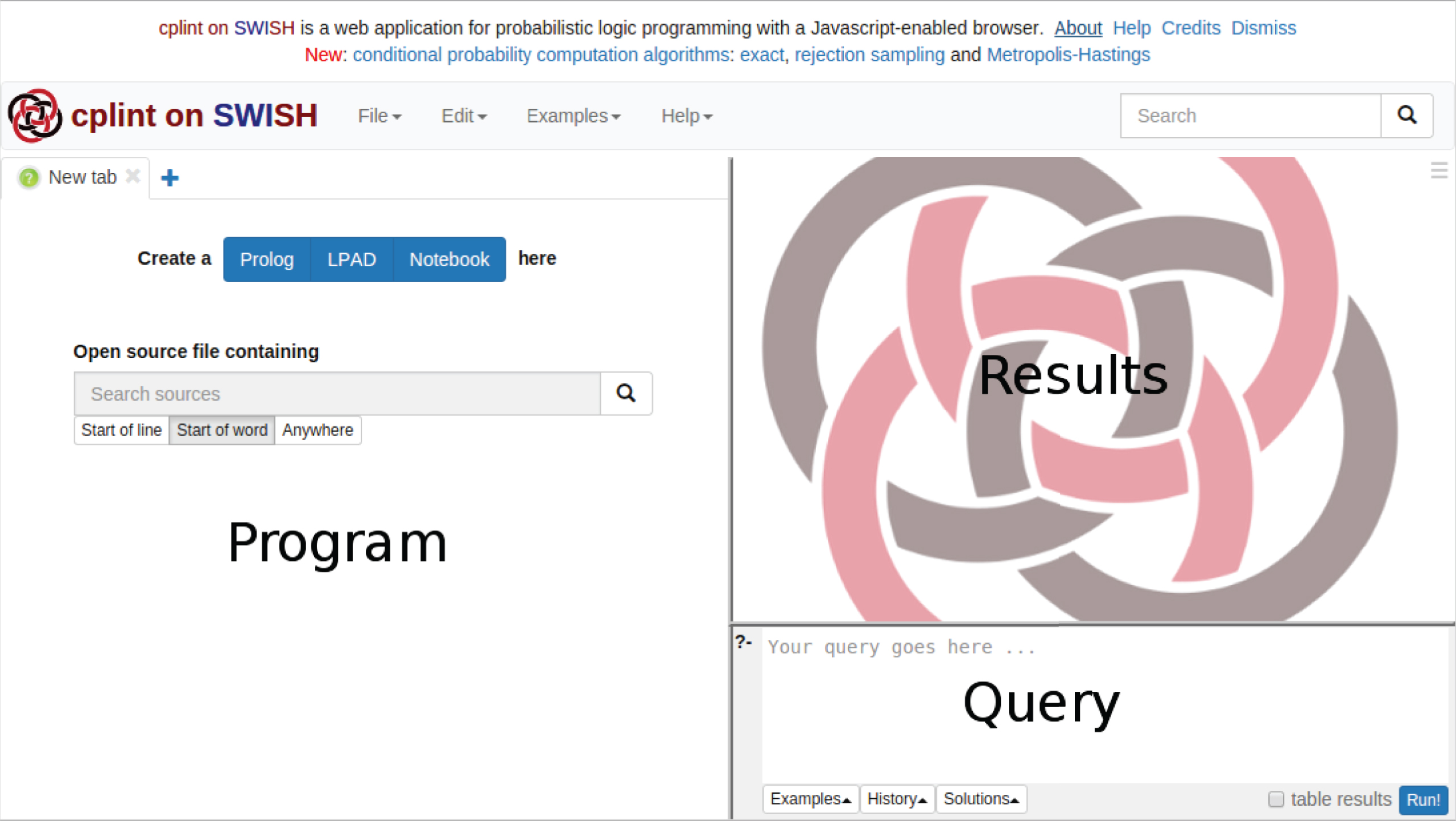
Many systems have been proposed for reasoning with PLP, most of them freely available. However, in many cases the installation process of these systems is prone to errors and they require that one must follow a non-trivial learning phase before becoming a proficient user. In order to facilitate the use of our PLP systems, we developed cplint on SWISH [17], a web application for reasoning on PLP with just a web browser. The application is available at http://cplint.lamping.unife.it and Fig. 1 shows its interface. Here, users have just to use their browser to post queries and see the results, while all the execution is demanded to a web server.

Fig.1

Interface of cplint on SWISH.

cplint on SWISH uses the reasoning algorithms included in the cplint suite, including exact and approximate inference and parameter and structure learning. This article extends [1], where we presented several algorithms for computing conditional probabilities with exact, rejection sampling and Metropolis-Hasting methods. The system also allowed hybrid programs, where some of the random variables are continuous, a feature that is, to the best of our knowledge, a novelty for web applications.

A similar system is ProbLog2 [7], which also has an online version 1 . The main difference between cplint on SWISH and ProbLog2 is that the former currently offers also structure learning, approximate conditional inference through sampling and handling of continuous variables. Moreover, cplint on SWISH is based on SWISH 2 - a web framework for Logic Programming using features and packages of SWI-Prolog and its Pengines library - and utilizes a Prolog-only software stack in the server, whereas ProbLog2 relies on several different technologies, including Python 3 and the DSHARP compiler. In particular, it writes intermediate files to disk in order to call external programs such as DSHARP, while we work in main memory only.

In this paper we aim to show that PP based on Logic Programming is flexible and mature enough to develop complex systems equipped with many features and algorithms with relative ease. PLP has moved from a niche language suitable for specific applications to a versatile framework able to offer many features that were previously typical of imperative or functional PP languages only, such as hybrid programs, likelihood weighting and particlefiltering.

cplint on SWISH not only offers such features but also the possibility of developing programs online and in collaboration. The system contains a wide variety of examples, representing many probabilistic models such as Markov Logic Networks, generative models, Gaussian processes, Gaussian mixtures, Dirichlet processes, Bayesian estimation and Kalman filters. As such, the system shows the soundness of PLP also from a software engineering point of view, opening the way to complex industrial/real world applications.

After introducing the syntax and semantics of PLP in Section 2, we discuss approaches for inference in Section 3. Section 4 presents the predicates the user can call to perform inference in cplint on SWISH. Section 5 contains a number of examples that illustrate the new features of cplint on SWISH and Section 6 concludes the paper. All the examples presented in the paper named as <name>.pl can be accessed online at http://cplint.lamping.unife.it/example/inference/<name>.pl.

2 Syntax and semantics

The distribution semantics [23] is one of the most used approaches for representing probabilistic information in Logic Programming and it is at the basis of many languages, such as Independent Choice Logic, PRISM, Logic Programs with Annotated Disjunctions (LPADs) and ProbLog.

We consider first the discrete version of probabilistic logic programming languages. In this version, each atom is a Boolean random variable that can assume values true or false. Facts and rules of the program specify the dependences among the truth value of atoms and the main inference task is to compute the probability that a ground query is true, often conditioned on the truth of another ground goal, the evidence. All the languages following the distribution semantics allow the specification of alternatives either for facts and/or for clauses. We present here the syntax of LPADs because it is the most general [25]. An LPAD is a finite set of annotated disjunctive clauses of the form h_i1 : Π_i1 ; … ; h_{in
_i} : Π_{in
_i} : - b_i1, …, b_{im
_i} . where b_i1, …, b_{im
_i} are literals, h_i1, … h_{in
_i} are atoms and Π_i1, …, Π_{in
_i} are real numbers in the interval [0, 1]. This clause can be interpreted as “if b_i1, …, b_{im
_i} is true, then h_i1 is true with probability Π_i1 or …or h_{in
_i} is true with probability Π_{in
_i}.”

Given an LPAD P, the grounding ground (P) is obtained by replacing variables with terms from the Herbrand universe in all possible ways. If P does not contain function symbols and P is finite, ground (P) is finite as well.

ground (P) is still an LPAD from which, by selecting a head atom for each ground clause, we can obtain a normal logic program, called “world”, to which we can assign a probability by multiplying the probabilities of all the head atoms chosen. In this way we get a probability distribution over worlds from which we can define a probability distribution over the truth values of a ground atom: the probability of an atom q being true is the sum of the probabilities of the worlds where q is true, that can be checked because the worlds are normal programs that we assume have a two-valued well-founded model.

This semantics can be given also a sampling interpretation: the probability of a query q is the fraction of worlds, sampled from the distribution over worlds, where q is true. To sample from the distribution over worlds, you simply randomly select a head atom for each clause according to the probabilistic annotations. Note that you don’t even need to sample a complete world: if the samples you have taken ensure the truth value of q is determined, you don’t need to sample more clauses.

To compute the conditional probability P (q|e) of a query q given evidence e, you can use the definition of conditional probability, P (q|e) = P (q, e)/P (e), and compute first the probability of q, e (the sum of probabilities of worlds where both q and e are true) and the probability of e and then divide the two.

If the program P contains function symbols, a more complex definition of the semantics is necessary, because ground (P) is infinite, a world would be obtained by making an infinite number of choices and so its probability, the product of infinite numbers all smaller than one, would be 0. In this case you have to work with sets of worlds and use Kolmogorov’s definition of probability space [21].

Up to now we have considered only discrete random variables and discrete probability distributions. How can we consider continuous random variables and probability density functions, for example real variables following a Gaussian distribution? cplint allows the specification of density functions over arguments of atoms in the head of rules. Forexample, in

$g (X, Y) : gaussian (Y, 0, 1) : - object (X) .$ X takes terms while Y takes real numbers as values. The clause states that, for each X such that object(X) is true, the values of Y such that g(X,Y) is true follow a Gaussian distribution with mean 0 and variance 1. You can think of an atom such as g(a,Y) as an encoding of a continuous random variable associated to term g(a). A semantics to such programs was given independently in [8] and [9]. In [14] the semantics of these programs, called Hybrid Probabilistic Logic Programs (HPLP), is defined by means of a stochastic generalization STp of the Tp operator that applies to continuous variables the sampling interpretation of the distribution semantics: STp is applied to interpretations that contain ground atoms (as in standard logic programming) and terms of the form t = v where t is a term indicating a continuous random variable and v is a real number. If the body of a clause is true in an interpretation I, STp (I) will contain a sample from the head.

In [9] a probability space for N continuous random variables is defined by considering the Borel σ-algebra over $ℝ^{N}$ and a Lebesgue measure on this set as the probability measure. The probability space is lifted to cover the entire program using the least model semantics of constraint logic programs.

If an atom encodes a continuous random variable (such as g(X,Y) above), asking the probability that a ground instantiation, such as g(a,0.3), is true is not meaningful, as the probability that a continuous random variables takes a specific value is always 0. In this case you are more interested in computing the distribution of Y of a goal g(a,Y), possibly after having observed some evidence. If the evidence is on an atom defining another continuous random variable, the definition of conditional probability cannot be applied, as the probability of the evidence would be 0 and so the fraction would be undefined. This problem is resolved in [14] by providing a definition using limits.

3 Inference

Computing all the worlds is impractical because their number is exponential in the number of ground probabilistic clauses. Alternative approaches have been considered that can be grouped in exact and approximate ones.

For exact inference from discrete programs without function symbols a successful approach finds explanations for the query q [3], where an explanation is a set of clause choices that are sufficient for entailing the query. Once all explanations for the query are found, they are encoded as a Boolean formula in DNF (with a propositional variable per choice and a conjunction per explanation) and the problem is reduced to that of computing the probability that a propositional formula is true. This problem is difficult (#P complexity) but converting the DNF into a language from which the computation of the probability is polynomial (knowledge compilation [4]) yields algorithms able to handle problems of significant size [3, 22]. One of the most efficient ways of solving the problem makes use of the language of Binary Decision Diagrams (BDDs). They represent a function f (X) taking Boolean values on a set of Boolean variables X by means of a rooted graph that has one level for each variable. Each node is associated with the variable of its level and has 2 children. Given values for all the variables, we can compute the value of the function (in this case the DNF formula) by traversing the graph from the root and returning the value associated with the leaf that is reached: the diagram will have a path to a 1-leaf for each world where the query is true.

Given a BDD, the probability of the corresponding Boolean function can be computed with a dynamic programming algorithm. The probability of a leaf is either 1 or 0 if the leaf is 1 or 0 respectively. The probability P (n) of a node n associated with variable V is P (n) = P (V) · P (child₁ (n)) + (1 - P (V)) · P (child₀ (n)) where child₁ (n) (child₀ (n)) is the 1-child (0-child) of n. In practice, memorization of intermediate results is used to avoid recomputation at nodes that are shared between multiple paths.

For approximate inference one of the most used approach consists in Monte Carlo sampling, following the sampling interpretation of the semantics given above. Monte Carlo backward reasoning has been implemented in [10, 20] and found to give good performance in terms of quality of the solutions and of running time. Monte Carlo sampling is attractive for the simplicity of its implementation and because you can improve the estimate as more time is available. Moreover, Monte Carlo can be used also for programs with function symbols, in which goals may have infinite explanations and exact inference may loop. In sampling, infinite explanations have probability 0, so the computation of each sample eventually terminates.

Monte Carlo inference provides also smart algorithms for computing conditional probabilities: rejection sampling or Metropolis-Hastings Markov Chain Monte Carlo (MCMC). In rejection sampling [24], you first query the evidence and, if the query is successful, query the goal in the same sample, otherwise the sample is discarded. In Metropolis-Hastings MCMC [15], a Markov chain is built by taking an initial sample and by generating successor samples.

The initial sample is built by randomly sampling choices so that the evidence is true. A successor sample is obtained by deleting a fixed number of sampled probabilistic choices. Then the evidence is queried by taking a sample starting with the undeleted choices. If the query succeeds, the goal is queried by taking a sample. The sample is accepted with a probability of $min {1, \frac{N_{0}}{N_{1}}}$ where N₀ is the number of choices sampled in the previous sample and N₁ is the number of choices sampled in the current sample. Then the number of successes of the query is increased by 1 if the query succeeded in the last accepted sample. The final probability is given by the number of successes over the number of samples.

When you have evidence on ground atoms that have continuous values as arguments, you can still use Monte Carlo sampling. You cannot use rejection sampling or Metropolis-Hastings, as the probability of the evidence is 0, but you can use likelihood weighting [14] to obtain samples of continuous arguments of a goal.

For each sample to be taken, likelihood weighting samples the query and then assigns a weight to the sample on the basis of evidence. The weight is computed by deriving the evidence backward in the same sample of the query starting with a weight of one: each time a choice should be taken or a continuous variable sampled, if the choice/variable has already been taken, the current weight is multiplied by the probability of the choice/by the density value of the continuous variable.

If likelihood weighting is used to find the posterior density of a continuous random variable, you obtain a set of samples for the variables with each sample associated with a weight that can be interpreted as a relative frequency. The set of samples without the weight, instead, can be interpreted as the prior density of the variable. These two sets of samples can be used to plot the density before and after observing the evidence.

When you have a dynamic model and observations on continuous variables for a number of time points, or your evidence is represented by many atoms,likelihood weighting has numerical stability problems, as samples’ weight goes rapidly to 0. In this case, particle filtering can be useful, because it periodically resamples the individual samples/particles so that their weight is reset to 1.

You can sample arguments of queries also for discrete goals: in this case you get a discrete distribution over the values of one or more arguments of a goal. If the query predicate is determinate in each world, i.e., given values for input arguments there is a single value for output arguments that make the query true, you get a single value for each sample. Moreover, if clauses sharing an atom in the head are mutually exclusive, i.e., in each world the body of at most one clause is true, then the query defines a probability distribution over output arguments. In this way we can simulate those languages such as PRISM and Stochastic Logic Programs that define probability distributions over arguments rather than probability distributions over truth values of ground atoms.

4 Inference with cplint

cplint on SWISH uses two modules for performing inference, pita for exact inference by knowledge compilation and mcintyre for approximate inference by sampling. In this section we discuss the algorithms and predicates provided by these two modules.

The unconditional probability of an atom can be asked using pita with the predicate $\begin{matrix} prob (: Query : atom, - Probability : float) . \end{matrix}$ The conditional probability of a query atom given an evidence atom can be asked with the predicate

$\begin{matrix} prob (: Query : atom, : Evidence : atom, - Probability : float) . \end{matrix}$ The BDD representation of the explanations for the query atom can be obtained with the predicate

$\begin{matrix} bdd_d ot_s tring (: Query : atom, BDD : string, Var : list) . \end{matrix}$ With mcintyre, you can estimate the probability of a goal by taking a given number of samples using the predicate $\begin{matrix} mc_s ample (: Query : atom, + Samples : int, \\ - Probability : float) . \end{matrix}$ Moreover, you can sample arguments of querieswith:

$\begin{matrix} mc_s ample_a rg (: Query : atom, + Samples : int, \\ ? Arg : var, - Values : list) . \end{matrix}$ that returns in Values a list of couples V-W where L is the list of values of Arg for which Query succeeds in a world sampled at random and N is the number of samples returning that list of values. The version

$\begin{matrix} mc_s ample_a rg_f irst (: Query : atom, + Samples : int, \\ ? Arg : var, - Values : list) . \end{matrix}$ also samples arguments of queries but just computes the first answer of the query for each sampledworld.

You can ask conditional queries with rejection sampling or with Metropolis-Hastings MCMC, too. In the first case, the available predicate is: $\begin{matrix} mc_r ejection_s ample (: Query : atom, : Evidence : atom, \\ + Samples : int, - Successes : int, - Failures : int, \\ - Probability : float) . \end{matrix}$ In the second case, mcintyre follows the algorithm proposed in [15] (the non adaptive version). The initial sample is built with a backtracking meta-interpreter that starts with the goal and randomizes the order in which clauses are selected during the search so that the initial sample is unbiased. Then the goal is queried using regular mcintyre. A successor sample is obtained by deleting a number of sampled probabilistic choices given by the parameter lag. Then the evidence is queried using regular mcintyre starting with the undeleted choices. If the query succeeds, the goal is queried using regular mcintyre. The sample is accepted with the probability indicated in Section 3.

In [15] the lag is always 1. However, in [15], the proof that the acceptance probability (which is $min {1, \frac{N_{0}}{N_{1}}}$ where N₀ is the number of choices sampled in the previous sample and N₁ is the number of choices sampled in the current sample) yields a valid Metropolis-Hastings algorithm holds also when forgetting more than one sampled choice, so the lag is user-defined in cplint.

You can take a given number of samples with Metropolis-Hastings MCMC using $\begin{matrix} mc_m h_s ample (: Query : atom, : Evidence : atom, Samples : int, \\ + Lag : int, - Successes : int, - Failures : int, \\ - Probability : float) . \end{matrix}$ Moreover, you can sample the arguments of the queries with rejection sampling and Metropolis-Hastings MCMC using $\begin{matrix} mc_r ejection_s ample_a rg (: Query : atom, : Evidence : atom, \\ + Samples : int, ? Arg : var, - Values : list) . \\ mc_m h_s ample_a rg (: Query : atom, : Evidence : atom, \\ + Samples : int, + Lag : int, ? Arg : var, - Values : list) . \end{matrix}$ Finally, you can compute expectations with $\begin{matrix} mc_e xpectation (: Query : atom, + N : int, ? Arg : var, \\ - Exp : float) . \end{matrix}$ that returns the expected value of the argument Arg in Query by sampling. It takes N samples of Query and sums up the value of Arg in each sample. The overall sum is divided by N to give Exp.

To compute conditional expectations, use $\begin{matrix} mc_m h_e xpectation (: Query : atom, : Evidence : atom, \\ + N : int, + Lag : int, ? Arg : var, - Exp : float) . \end{matrix}$ For visualizing the results of sampling arguments you can use $\begin{matrix} mc_s ample_a rg_b ar (: Query : atom, + Samples : int, \\ ? Arg : var, - Chart : dict) . \\ mc_r ejection_s ample_a rg_b ar (: Quey : atom, \\ : Evidence : atom, + Samples : int, \\ ? Arg : var, - Chart : dict) . \\ mc_m h_s ample_a rg_b ar (: Query : atom, : Evidence : atom, \\ + Samples : int, + Lag : int, \\ ? Arg : var, - Chart : dict) . \end{matrix}$ that return in Chart a bar chart with a bar for each possible sampled value whose size is the number of samples returning that value.

When you have continuous random variables, you may be interested in sampling arguments of goals representing continuous random variables. In this way you can build a probability density of the sampled argument. When you do not have evidence or you have evidence on atoms not depending on continuous random variables, you can use the above predicates for sampling arguments.

When you have evidence on ground atoms with continuous values as arguments, you need to use likelihood weighting [14] or particle filtering [6, 11] to obtain samples of the continuous arguments of a goal.

For each sample to be taken, likelihood weighting uses a meta-interpreter to find a sample where the goal is true, randomizing the choice of clauses when more than one resolves with the goal, in order to obtain an unbiased sample. This meta-interpreter is similar to the one used to generate the first sample in Metropolis-Hastings.

Then a different meta-interpreter is used to evaluate the weight of the sample. This meta-interpreter starts with the evidence as the query and a weight of 1. Each time the meta-interpreter encounters a probabilistic choice over a continuous variable, it first checks whether a value has already been sampled. If so, it computes the probability density of the sampled value and multiplies the weight by it. If the value had not been sampled, it takes a sample and records it, leaving the weight unchanged. In this way, each sample in the result has a weight that is 1 for the prior distribution and that may be different from the posterior distribution, reflecting the influence of evidence.

The predicate $\begin{matrix} mc_l w_s ample_a rg (: Query : atom, : Evidence : atom, \\ + N : int, ? Arg : var, - ValList : list) . \end{matrix}$ returns in ValList a list of couples V-W where V is a value of Arg for which Query succeeds and W is the weight computed by likelihood weighting according to Evidence (a conjunction of atoms is allowed here).

In particle filtering, the evidence is a list of atoms. Each sample is weighted by the likelihood of an element of the evidence and constitutes a particle. After weighting, particles are resampled and the next element of the evidence is considered.

The predicate $\begin{matrix} mc_p article_s ample_a rg (: Query : atom, + Evidence : term, \\ + Samples : int, ? Arg : var, - Values : list) . \end{matrix}$ samples the argument Arg of Query using particle filtering given that Evidence is true. Evidence is a list of goals and Query can be either a single goal or a list of goals.

When Query is a single goal, the predicate returns in Values a list of couples V-W where V is a value of Arg for which Query succeeds in a particle in the last set of particles, and W is the weight of the particle. For each element of Evidence, the particles are obtained by sampling Query in each current particle and weighting the particle by the likelihood of the evidence element.

When Query is a list of goals, Arg is a list of variables, one for each query of Query; in this case Arg and Query must have the same length as Evidence. Values is then a list of the same length as Evidence and each of its elements is a list of couples V-W where V is a value of the corresponding element of Arg for which the corresponding element of Query succeeds in a particle, and W is the weight of the particle. For each element of Evidence, the particles are obtained by sampling the corresponding element of Query in each current particle and weighting the particle by the likelihood of the evidence element.

You can use the samples to draw the probability density function of the argument. The predicate $histogram (+ List : list, + NBins : int, - Chart : dict) .$ draws a histogram of the samples in List dividing the domain in NBins bins. List must be a list of couples of the form [V]-W where V is a sampled value and W is its weight. This is the format of the list of samples returned by argument sampling predicates except mc_lw_sample_arg/5, that returns a list of couples V-W. In this case you can use $\begin{matrix} densities (+ PriorList : list, + PostList : list, \\ + NBins : int, - Chart : dict) . \end{matrix}$ that draws a line chart of the density of two sets of samples, usually prior and post observations. The samples from the prior are in PriorList as couples [V]-W, while the samples from the posterior are in PostList as couples V-W where V is a value and W its weight. The lines are drawn dividing the domain in NBins bins.

5 Examples

5.1 Binary decision diagrams

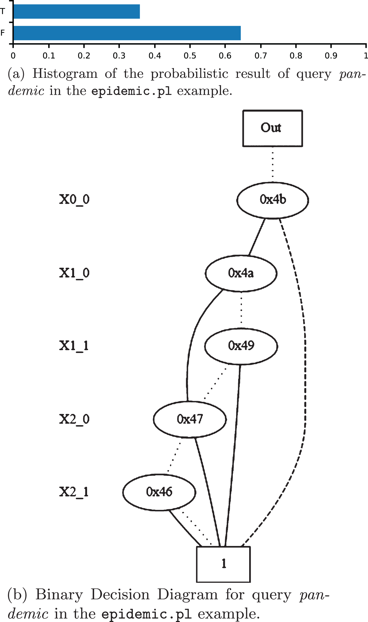
Example (http://cplint.lamping.unife.it/example/inference/epidemic.pl) models the development of an epidemic or a pandemic with an LPAD: if somebody has the flu and the climate is cold, there is the possibility that an epidemic arises with probability 0.6 and the possibility that a pandemic arises with probability 0.3, whereas with 0.1 probability neither an epidemic nor a pandemic arises. We are uncertain whether the climate is cold but we know for sure that David and Robert have the flu.

$\begin{matrix} epidemic : 0.6; pandemic : 0.3 : - flu (_), cold . \\ cold : 0.7 . \\ flu (david) . \\ flu (robert) . \end{matrix}$

In order to calculate the probability that a pandemic arises, you can call the query: $? - prob (pandemic, Prob) .$ or $? - prob_b ar (pandemic, Prob) .$ The latter shows the probabilistic results of the query as a histogram (Fig. 2a).

Fig.2

Graphical representations for query pandemic in epidemic.pl.

The corresponding BDD can be obtained with:

$? - bdd_d ot_s tring (pandemic, BDD, Var) .$ and is represented in Fig. 2b. A solid edge indicates a 1-child, a dashed edge indicates a 0-child and a dotted edge indicates a negated 0-child. Each level of the BDD is associated with a variable of the form X_IJ indicated on the left: I indicates the multivalued variable index and J the index of the Boolean variable of I.

5.2 Markov logic networks

Markov Networks (MNs) and Markov Logic Networks (MLNs)[19] can be encoded with Probabilistic Logic Programming. The encoding is based on the observation that a MN factor can be represented with a Bayesian Network with an extra node that is always observed. In order to model MLN formulas with LPADs, we can add an extra atom clause_i (X) for each formula F_i = w_i C_i where w_i is the weight associated with C_i and X is the vector of variables appearing in C_i. Then, when we ask for the probability of query q given evidence e, we have to ask for the probability of q given e ∧ ce, where ce is the conjunction of the groundings of clause_i (X) for all values of i. Then, clause C_i should be transformed into a Disjunctive Normal Form formula C_i1 ∨ … ∨ C_{in
_i}, where the disjuncts are mutually exclusive and the LPAD should contain the clauses clause_i (X) : e^α/(1 + e^α) ← C_ij for all j in 1, . . . , n_i. Similarly, ¬C_i should be transformed into a disjoint sum D_i1 ∨ … ∨ D_{im
_i} and the LPAD should contain the clauses clause_i (X) :1/(1 + e^α) ← D_il for all l in 1, . . . , m_i.

Alternatively, if α is negative, e^α will be smaller than 1 and we can use the two probability values e^α and 1 with the clauses clause_i (X) : e^α ← C_ij … clause_i (X) ← D_il . This solution has the advantage that some clauses are certain, reducing the number of random variables. If α is positive in the formula α C, we can consider the equivalent formula -α ¬ C.

MLN formulas can also be added to a regular probabilistic logic program, their effect being equivalent to a soft form of evidence, where certain worlds are weighted more than others. This is similar to soft evidence in Figaro [16].

The transformation above is illustrated by the following example. Here, ≅ indicates the truncation function. Given the MLN $\begin{matrix} 1.5 Intelligent (x) = > GoodMarks (x) \\ 1.1 Friends (x, y) = > (Intelligent (x) < = > Intelligent (y)) \end{matrix}$ the first formula is translated into the clauses: $\begin{matrix} clause 1 (X) : 0.8175 : - + intelligent (X) . \\ clause 1 (X) : 0.1824 : - intelligent (X), \\ + good_m arks (X) . \\ clause 1 (X) : 0.8175 : - intelligent (X), good_m arks (X) . \end{matrix}$

where 0.8175 ≅ e^1.5/(1 + e^1.5) and 0.1824 ≅ 1/(1 + e^1.5).

The second formula is translated into the clauses $\begin{matrix} clause 2 (X, Y) : 0.7502 : - + friends (X, Y) . \\ clause 2 (X, Y) : 0.7502 : - friends (X, Y), \\ intelligent (X), \\ intelligent (Y) . \\ clause 2 (X, Y) : 0.7502 : - friends (X, Y), \\ + intelligent (X), \\ + intelligent (Y) . \\ clause 2 (X, Y) : 0.2497 : - friends (X, Y), \\ intelligent (X), \\ + intelligent (Y) . \\ clause 2 (X, Y) : 0.2497 : - friends (X, Y), \\ + intelligent (X), \\ intelligent (Y) . \end{matrix}$ where 0.7502 ≅ e^1.1/(1 + e^1.1) and 0.2497 ≅ 1/(1 + e^1.1).

A priori we have a uniform distribution over student intelligence, good marks and friendship: $\begin{matrix} intelligent (_) : 0.5 . \\ good_m arks (_) : 0.5 . \\ friends (_,_) : 0.5 . \end{matrix}$ and there are two students: $\begin{matrix} student (anna) . \\ student (bob) . \end{matrix}$ We have evidence that Anna is friend with Bob and Bob is intelligent. The evidence must also include the truth of all groundings of the clause_N predicates: $\begin{matrix} evidence_m \ln : - clause 1 (anna), clause 1 (bob), \\ clause 2 (anna, anna), clause 2 (anna, bob), \\ clause 2 (bob, anna), clause 2 (bob, bob) . \\ ev_i ntelligent_b ob_f riends_a nna_b ob : - \\ intelligent (bob), friends (anna, bob), \\ evidence_m \ln . \end{matrix}$ If we want to query the probability that Anna gets good marks given the evidence, we can ask: $\begin{matrix} ? - prob (good_m arks (anna), \\ ev_i ntelligent_b ob_f riends_a nna_b ob, P) . \end{matrix}$

while the prior probability of Anna getting good marks is given by: $\begin{matrix} ? - prob (good_m arks (anna), evidence_m \ln, P) . \end{matrix}$ The probability resulting from the first query is higher (P = 0.733) than the second query (P = 0.607), since it is conditioned to the evidence that Bob is intelligent and Anna is her friend.

In the alternative transformation, the first MLN formula is translated into: $\begin{matrix} clause 1 (X) : - + intelligent (X) . \\ clause 1 (X) : 0.2231 : - intelligent (X), + good_m arks (X) . \\ clause 1 (X) : - intelligent (X), good_m arks (X) . \end{matrix}$ where 0.2231 ≅ e^-1.5.

5.3 Generative model

Program (http://cplint.lamping.unife.it/example/inference/arithm.pl) encodes a model for generating random functions: $\begin{matrix} eval (X, Y) : - random_f n (X, 0, F), Y is F . \\ op (+) : 0.5; op (-) : 0.5 . \\ random_f n (X, L, F) : - comb (L), random_f n (X, l (L), F 1), \\ random_f n (X, r (L), F 2), op (Op), F = . . [Op, F 1, F 2] . \\ random_f n (X, L, F) : - + comb (L), base_r andom_f n (X, L, F) . \\ comb (_) : 0.3 . \\ base_r andom_f n (X, L, X) : - identity (L) . \\ base_r andom_f n (_, L, C) : - + identity (L), \\ random_c onst (L, C) . \\ identity (_) : 0.5 . \\ random_c onst (_, C) : discrete (C, [0 : 0.1, 1 : 0.1, 2 : 0.1, \\ 3 : 0.1, 4 : 0.1, 5 : 0.1, 6 : 0.1, 7 : 0.1, 8 : 0.1, 9 : 0.1]) . \end{matrix}$ A random function is either an operator (‘+’ or ‘-’) applied to two random functions or a base random function. A base random function is either an identity or a constant drawn uniformly from the integers 0, …, 9.

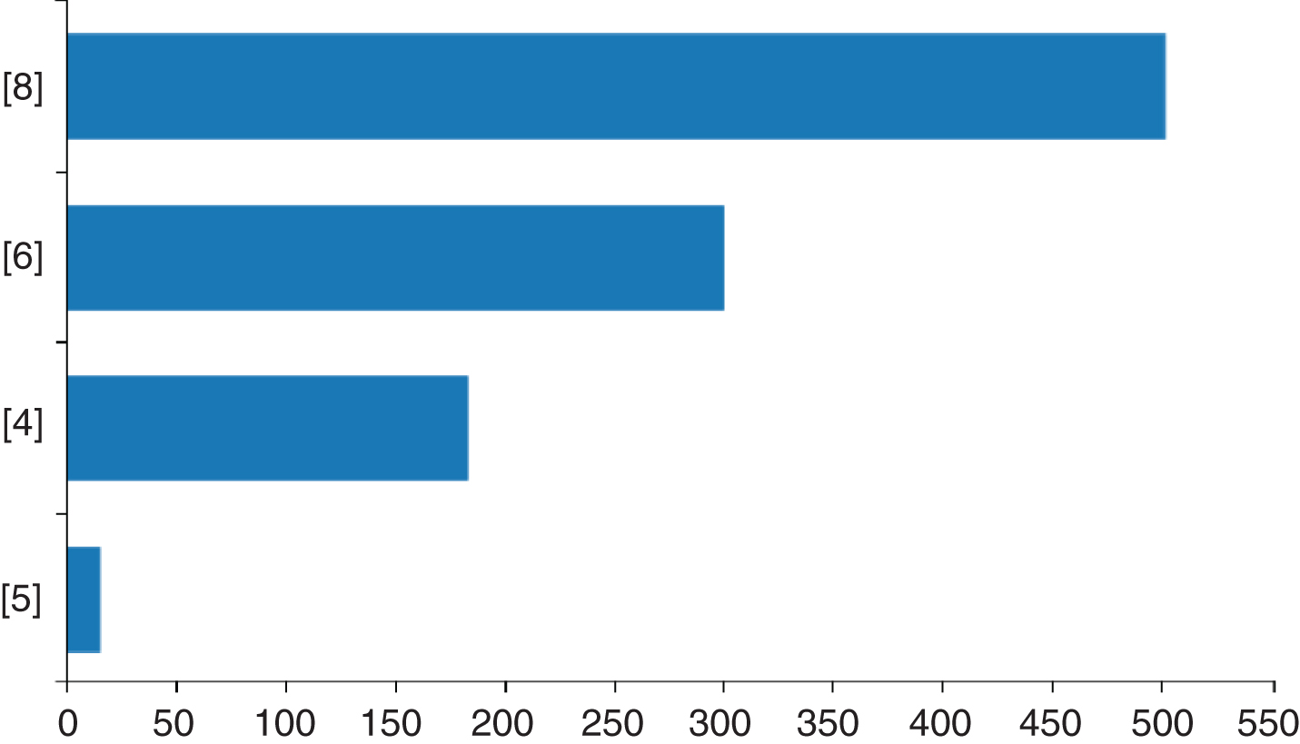
You may be interested in the distribution of the output values of the random function with input 2 given that the function outputs 3 for input 1. You can get this distribution with $\begin{matrix} ? - mc_m h_s ample_a rg_b ar (eval (2, Y), \\ eval (1, 3), 1000, 1, Y, V) . \end{matrix}$ that samples 1000 values for Y in eval(2,Y) and returns them in V. A bar graph of the frequencies of the sampled values is shown in Fig. 3.

Fig.3

Distribution of sampled values in the arithm.pl example.

Since each world of the program is determinate, in each world there is a single value of Y in eval(2,Y) and the list of sampled values contains a single element.

5.4 Gaussian Process

A Gaussian Process (GP) (example (http://cplint.lamping.unife.it/example/inference/gpr.pl) defines a probability distribution over functions. This distribution has the property that, given N values, their image through a function sampled from the gaussian process follows a multivariate normal with mean 0 and covariance matrix K. A Gaussian Process is defined by a kernel function k that determines K. GPs can be used for regression: the random functions predicts the y value corresponding to a x value given a set X and Y of observed values. When performing GP regression, you choose the kernel and you want to estimate the parameters of the kernel. You can define a prior distribution over the parameters. The following program can sample kernels (and thus functions) and compute the expected value of the predictions for a squared exponential kernel (defined by predicate sq_exp_p) with parameters l uniformly distributed in 1, 2, 3 and σ uniformly distributed in [-2, 2].

The predicate gp, given a list of values X and a kernel name, returns in Y the list of values of type f (x) where x belongs to X and f is a function sampled from the Gaussian process. gp_predict, given the points described by the lists XT and YT and a kernel, predict the Y values of points with X values in XP and returns them in YP. Prediction is performed by Gaussian process regression.

$\begin{array}{l} g p (X, K e r n e l, Y) : - \\ c o m p u t e_c o v (X, K e r n e l, 0, C), \\ g p (C, Y) . \\ g p (C o v, Y) : g a u s s i a n (Y, M e a n, C o v) : - \\ l e n g t h (C o v, N), \\ l i s t 0 (N, M e a n) . \\ c o m p u t e_c o v (X, K e r n e l, V a r, C) : - \\ l e n g t h (X, N), \\ c o v (X, N, K e r n e l, V a r, C T, C N D), \\ t r a n s p o s e (C N D, C N D T), \\ m a t r i x_s u m (C T, C N D T, C) . \\ c o v ([],_,_,_, [], []) . \\ c o v ([X H | X T], N, K e r, V a r, [K H | K Y], [K H N D | K Y N D]) : - \\ l e n g t h (X T, L X), \\ N 1 i s N - L X - 1, \\ l i s t 0 (N 1, K H 0), \\ c o v_r o w (X T, X H, K e r, K H 1), \\ c a l l (K e r, X H, X H, K X H 0), \\ K X H i s K X H 0 + V a r, \\ a p p e n d ([K H 0, [K X H], K H 1], K H), \\ a p p e n d ([K H 0, [0], K H 1], K H N D), \\ c o v (X T, N, K e r, V a r, K Y, K Y N D) . \\ c o v_r o w ([],_,_, []) . \\ c o v_r o w ([H | T], X H, K e r, [K H | K T]) : - \\ c a l l (K e r, H, X H, K H), \\ c o v_r o w (T, X H, K e r, K T) . \\ g p_p r e d i c t (X P, K e r n e l, V a r, X T, Y T, Y P) : - \\ c o m p u t e_c o v (X T, K e r n e l, V a r, C), \\ m a t r i x_i n v e r s i o n (C, C_1), \\ t r a n s p o s e ([Y T], Y S T), \\ m a t r i x_m u l t i p l y (C_1, Y S T, C_1 T), \\ g p_p r e d i c t_s i n g l e (X P, K e r n e l, X T, C_1 T, Y P) . \\ g p_p r e d i c t_s i n g l e ([],_,_,_, []) . \\ g p_p r e d i c t_s i n g l e ([X H | X T], K e r n e l, X, C_1 T, \\ [Y H | Y T]) : - \\ c o m p u t e_k (X, X H, K e r n e l, K), \\ m a t r i x_m u l t i p l y ([K], C_1 T, [[Y H]]), \\ g p_p r e d i c t_s i n g l e (X T, K e r n e l, X, C_1 T, Y T) . \\ c o m p u t e_k ([],_,_, []) . \\ c o m p u t e_k ([X H | X T], X, K e r, [H K | T K]) : - \\ c a l l (K e r, X H, X, H K), \\ c o m p u t e_k (X T, X, K e r, T K) . \\ s q_e x p_p (X, X P, K) : - \\ s i g m a (S i g m a), \\ l (L), \\ K i s S i g m a^{\land} 2 * e x p (- ({(X - X P)}^{\land} 2) / 2 / (L^{\land} 2)) . \\ c l (L) : u n i f o r m (L, [1, 2, 3]) . \\ s i g m a (S i g m a) : u n i f o r m (S i g m a, - 2, 2) . 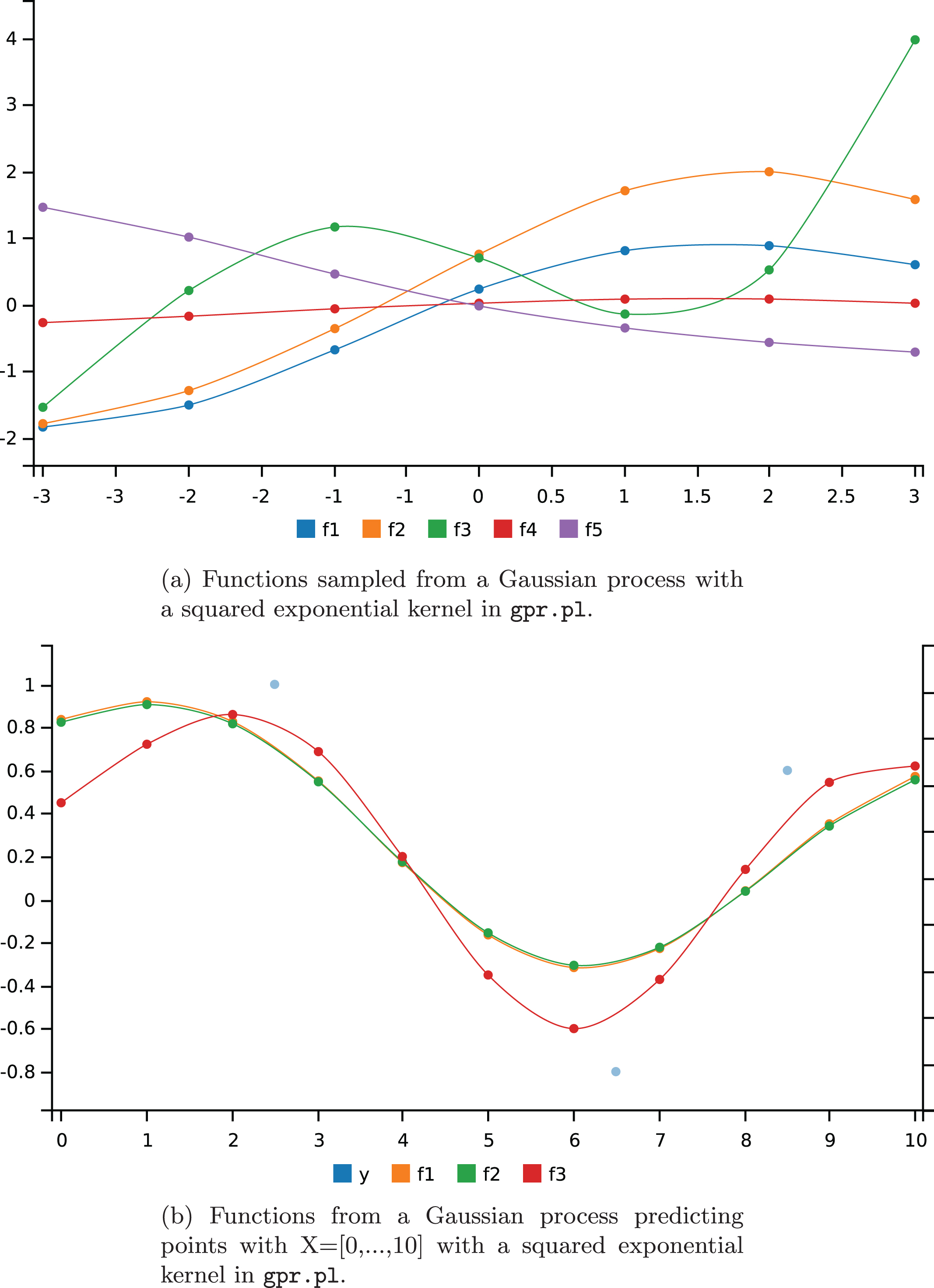\end{array}$ By calling the query ?-draw_fun(sq_exp_p,C). over the program: $\begin{matrix} draw_f un (Kernel, C) : - \\ X = [- 3, - 2, - 1, 0, 1, 2, 3], \\ draw_f un (X, Kernel, C) . \\ draw_f un (X, Kernel, C) : - \\ mc_s ample_a rg_f irst (gp (X, Kernel, Y), 5, Y, L) . \end{matrix}$

we get 5 functions sampled from the Gaussian process with a squared exponential kernel at points X = [-3, - 2, - 1, 0, 1, 2, 3], shown in Fig. 4a.

Fig.4

Functions sampled from a Gaussian Process in the gpr.pl example.

The query ?-draw_fun_pred(sq_exp_p,C). called over the program: $\begin{matrix} draw_f un_p red (Kernel, C) : - \\ numlist (0, 10, X), \\ XT = [2.5, 6.5, 8.5], \\ YT = [1, - 0.8, 0.6], \\ mc_l w_s ample_a rg (gp_p redict (X, Kernel, \\ 0.3, XT, YT, Y), gp (XT, Kernel, YT), 5, Y, L) . \end{matrix}$ draws 3 functions predicting points with X values in [0,...,10] given the three couples of points XT=[2.5,6.5,8.5], YT=[1,-0.8,0.6] with a squared exponential kernel. The graph (Fig. 4b) shows as dots the given points.

5.5 Gaussian mixture model

Example (http://cplint.lamping.unife.it/example/inference/gaussian_mixture.pl) defines a mixture of two Gaussians: $\begin{matrix} heads : 0.6; tails : 0.4 . \\ g (X) : gaussian (X, 0, 1) . \\ h (X) : gaussian (X, 5, 2) . \\ mix (X) : - heads, g (X) . \\ mix (X) : - tails, h (X) . \end{matrix}$

The argument X of mix(X) follows a model mixing two Gaussians, one with mean 0 and variance 1 with probability 0.6 and one with mean 5 and variance 2 with probability 0.4.

The query $\begin{matrix} ? - mc_s ample_a rg (mix (X), 10000, X, L 0), \\ histogram (L 0, 40, Chart) . \end{matrix}$ draws the density of the random variable X of mix(X), shown in Fig. 5.

Fig.5

Density of X of mix(X) in gaussian_mixture.pl.

5.6 Dirichlet processes

A Dirichlet process (DP) is a probability distribution whose range is itself a set of probability distributions. The DP is specified by a base distribution, which represents the expected value of the process. New samples have a nonzero probability of being equal to already sampled values. The process depends on a parameter α, called concentration parameter: with α → 0 a single value is sampled, with α→ ∞ the distribution is equal to the base distribution. There are several equivalent views of the Dirichlet process, that are presented in the following.

5.6.1 The stick-breaking process

Example (http://cplint.lamping.unife.it/example/inference/dirichlet_process.pl) encodes the stick-breaking process view of the DP.

In this example the base distribution is a Gaussian with mean 0 and variance 1. To sample a value, a sample β₁ is taken from the beta distribution Beta (1, α) and a coin with heads probability equal to β₁ is flipped. If the coin lands on heads, a sample from the base distribution is taken and returned. Otherwise, a sample β₂ is taken again from Beta (1, α) and a coin is flipped. This procedure is repeated until heads is obtained, the index i of β_i being the index of the value to be returned.

The distribution of values is handled by predicates dp_value/3, which returns in V the NVth sample from the DP with concentration parameter Alpha, and dp_n_values/4, which returns in L a list of N-N0 samples from the DP with concentration parameter Alpha.

The distribution of indexes is handled by predicates dp_stick_index. $\begin{matrix} dp_n_v alues (N, N,_A lpha, []) : -! . \\ dp_n_v alues (N 0, N, Alpha, [[V] - 1 | Vs]) : - \\ N 0 < N, \\ dp_v alue (N 0, Alpha, V), \\ N 1 is N 0 + 1, \\ dp_n_v alues (N 1, N, Alpha, Vs) . \\ dp_v alue (NV, Alpha, V) : - \\ dp_s tick_i ndex (NV, Alpha, I), \\ dp_p ick_v alue (I, V) . \\ dp_p ick_v alue (_, V) : gaussian (V, 0, 1) . \\ dp_s tick_i ndex (NV, Alpha, I) : - \\ dp_s tick_i ndex (1, NV, Alpha, I) . \\ dp_s tick_i ndex (N, NV, Alpha, V) : - \\ stick_p roportion (N, Alpha, P), \\ choose_p rop (N, NV, Alpha, P, V) . \\ choose_p rop (N, NV,_A lpha, P, N) : - \\ pick_p ortion (N, NV, P) . \\ choose_p rop (N, NV, Alpha, P, V) : - \\ neg_p ick_p ortion (N, NV, P), \\ N 1 is N + 1, \\ dp_s tick_i ndex (N 1, NV, Alpha, V) . \\ stick_p roportion (_, Alpha, P) : \\ beta (P, 1, Alpha) . \\ pick_p ortion (_,_, P) : P; \\ neg_p ick_p ortion (_,_, P) : 1 - P . \end{matrix}$ The query $\begin{matrix} ? - mc_s ample_a rg (dp_s tick_i ndex (1, 10.0, V), 200, V, L), \\ histogram (L, 100, Chart) . 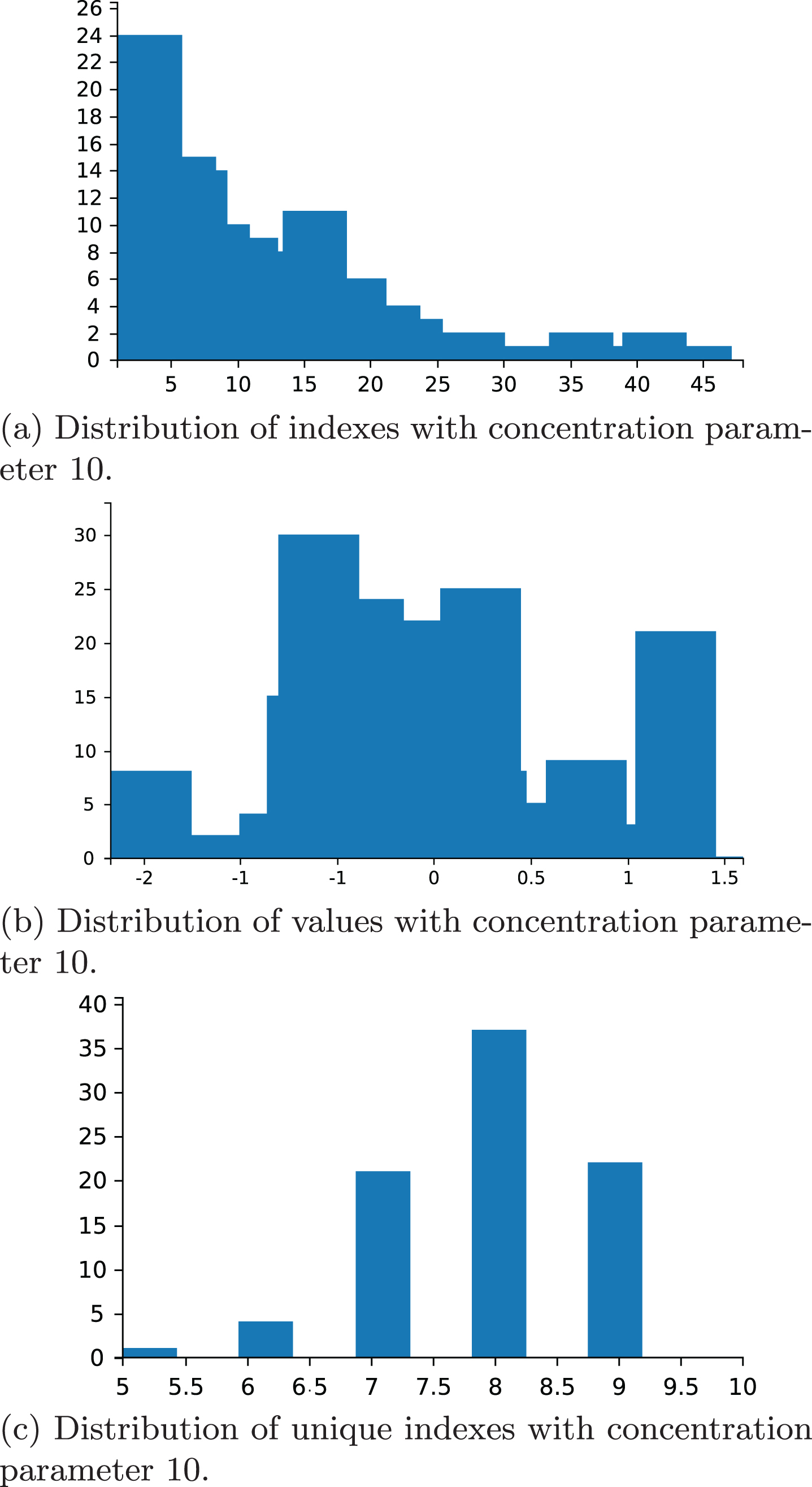\end{matrix}$ draws the density of indexes with concentration parameter 10 using 200 samples (Fig. 6a).

Fig.6

Representation of the distributions in the dirichlet_process.pl example.

The query $\begin{matrix} ? - mc_s ample_a rg_f irst (dp_n_v alues (0, 200, 10.0, V), 1, V, L), \\ L = [Vs -_], \\ histogram (Vs, 100, Chart) . \end{matrix}$ draws the density of values with concentration parameter 10 using 200 samples (Fig. 6b).

The query $\begin{matrix} ? - hist_r epeated_i ndexes (100, 40, G) . \end{matrix}$ called over the program: $\begin{matrix} hist_r epeated_i ndexes (Samples, NBins, Chart) : - \\ repeat_s ample (0, Samples, L), \\ histogram (L, NBins, Chart) . \\ repeat_s ample (S, S, []) : -! . \\ repeat_s ample (S 0, S, [[N] - 1 | LS]) : - \\ mc_s ample_a rg_f irst (dp_s tick_i ndex \\ (1, 1, 10.0, V), 10, V, L), \\ length (L, N), \\ S 1 is S 0 + 1, \\ repeat_s ample (S 1, S, LS) . \end{matrix}$ shows the distribution of unique indexes in 100 samples with concentration parameter 10 (Fig. 6c).

5.6.2 The Chinese restaurant process

The Chinese restaurant process is a discrete-time stochastic process, analogous to seating customers at tables in a Chinese restaurant. It results from considering the conditional distribution of one component assignment given all previous ones in a Dirichlet distribution mixture model with K components, and then taking the limit as K goes to infinity.

In the example (http://cplint.lamping.unife.it/example/inference/dp_chinese.pl) the base distribution is a Gaussian with mean 0 and variance 1. X₁ is drawn from the base distribution. For n > 1, with probability $\frac{α}{α + n - 1}$ X_n is drawn from the base distribution; with probability $\frac{n_{x}}{α + n - 1}$ X_n = x, where n_x is the number of previous observations X_j, j < n, such that X_j = x. Counts are kept by predicate update_counts/5. $\begin{matrix} dp_n_v alues (N 0, N, Alpha, [[V] - 1 | Vs], \\ Counts 0, Counts) : - \\ N 0 < N, \\ dp_v alue (N 0, Alpha, Counts 0, V, Counts 1), \\ N 1 is N 0 + 1, \\ dp_n_v alues (N 1, N, Alpha, Vs, Counts 1, Counts) . \\ dp_v alue (NV, Alpha, Counts, V, Counts 1) : - \\ draw_s ample (Counts, NV, Alpha, I), \\ update_c ounts (0, I, Alpha, Counts, Counts 1), \\ dp_p ick_v alue (I, V) . \\ update_c ounts (_I 0,_I, Alpha, [_C], \\ [1, Alpha]) : -! . \\ update_c ounts (I, I,_A lpha, [C | Rest], \\ [C 1 | Rest]) : - C 1 is C + 1 . \\ update_c ounts (I 0, I, Alpha, [C | Rest], \\ [C | Rest 1]) : - I 1 is I 0 + 1, \\ update_c ounts (I 1, I, Alpha, Rest, Rest 1) . \\ draw_s ample (Counts, NV, Alpha, I) : - \\ NS is NV + Alpha, \\ maplist (div (NS), Counts, Probs), \\ length (Counts, LC), \\ numlist (1, LC, Values), \\ maplist (pair, Values, Probs, Discrete), \\ take_s ample (NV, Discrete, I) . \\ take_s ample (_, D, V) : discrete (V, D) . \\ dp_p ick_v alue (_, V) : gaussian (V, 0, 1) . \\ div (Den, V, P) : - P is V / Den . \\ pair (A, B, A : B) . \end{matrix}$

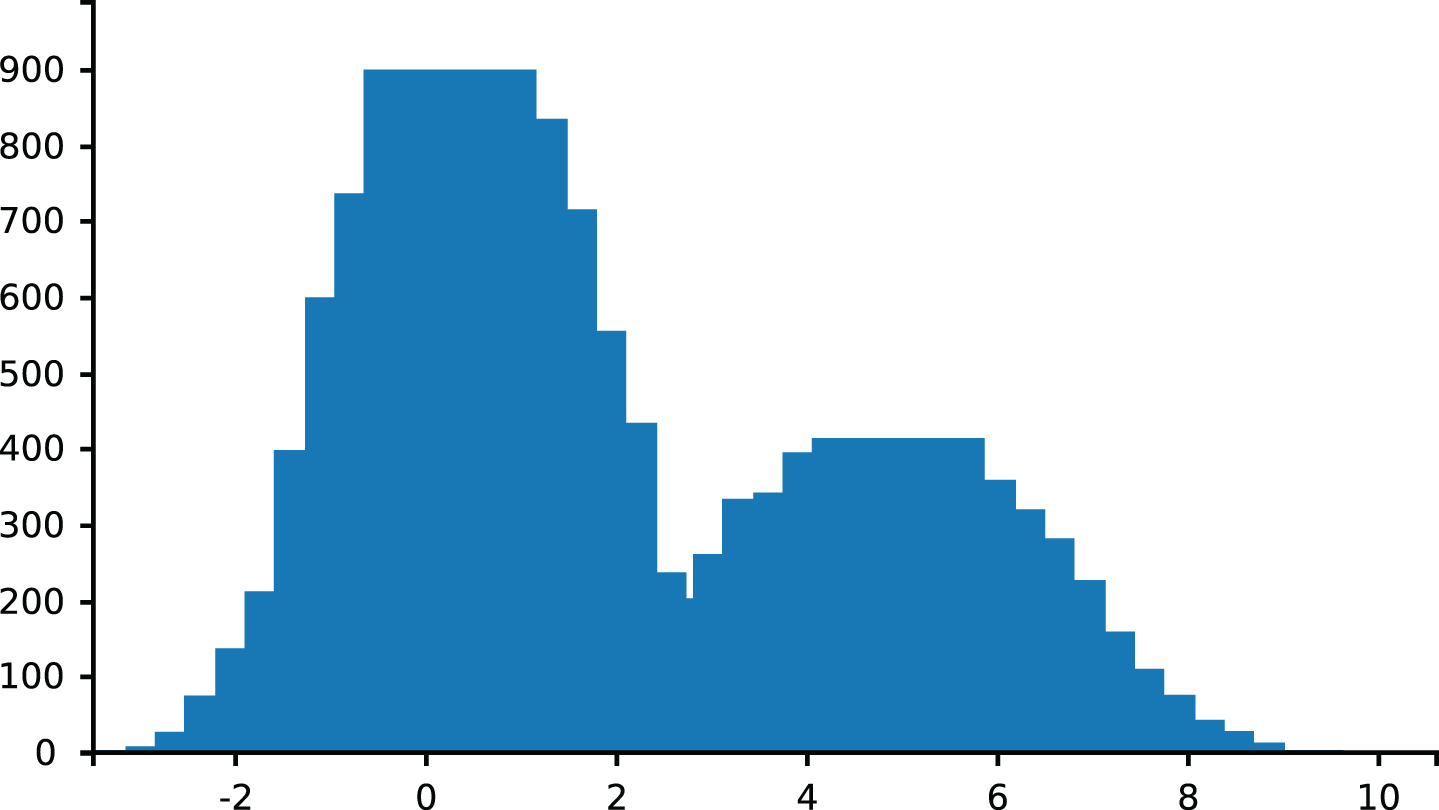
The query $\begin{matrix} ? - mc_s ample_a rg_f irst (dp_n_v alues \\ (0, 200, 10.0, V, [10.0],_), 1, V, L), \\ L = [Vs -_], \\ histogram (Vs, 100, Chart) . \end{matrix}$ draws the distribution of values with concentration parameter 10 using 200 samples (Fig. 7).

Fig.7

Distribution of values in the dp_chinese.pl example.

5.6.3 Mixture model

A particularly important application of Dirichlet processes is as a prior probability distribution in infinite mixture models. The target is to build a mixture model which does not require us to specify the number of k components from the beginning. In the example (http://cplint.lamping.unife.it/example/inference/dp_mix.pl) samples are drawn from a mixture of normal distributions whose parameters are defined by means of a Dirichlet process. For each component, the variance is sampled from a gamma distribution and the mean is sampled from a Gaussian with mean 0 and variance 30 times the variance of the component. The program in this case is equivalent to the one encoding the stick-breaking example, except for the dp_pick_value/3 predicate that is reported in the following.

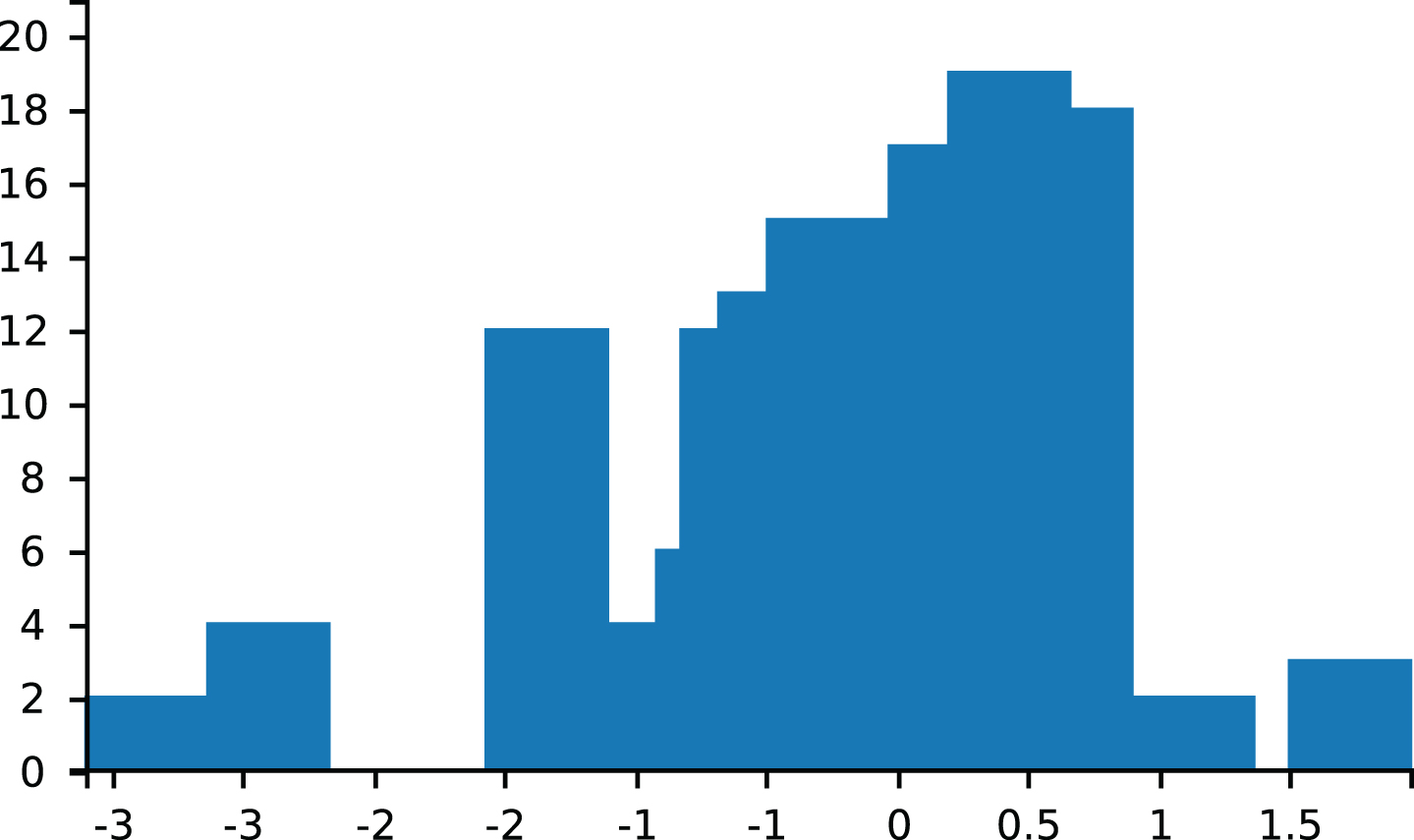
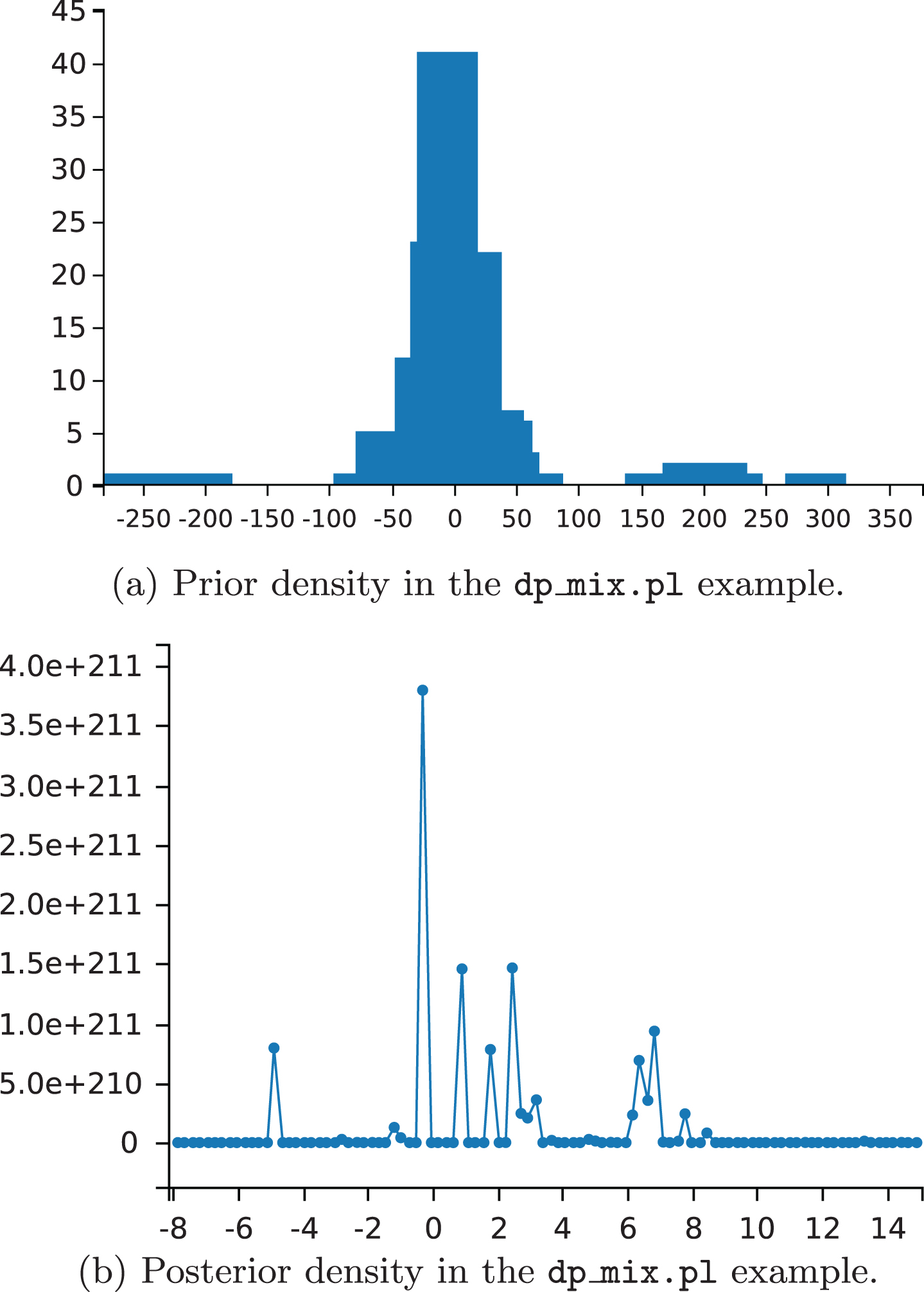
$\begin{matrix} dp_p ick_v alue (I, NV, V) : - \\ ivar (I, IV), \\ Var is 1.0 / IV, \\ mean (I, Var, M), \\ value (NV, M, Var, V) . \\ ivar (_, IV) : gamma (IV, 1, 0.1) . \\ mean (_, V 0, M) : gaussian (M, 0, V) : - V is V 0 * 30 . \\ value (_, M, V, Val) : gaussian (Val, M, V) . \end{matrix}$ Given a vector of observations obs([-1,7,3]), the queries

$\begin{matrix} ? - prior (200, 100, G) . \\ ? - post (200, 100, G) . \end{matrix}$ called over the program: $\begin{matrix} prior (Samples, NBins, Chart) : - \\ mc_s ample_a rg_f irst (dp_n_v alues \\ (0, Samples, 10.0, V), 1, V, L), \\ L = [Vs -_], \\ histogram (Vs, NBins, Chart) . \\ post (Samples, NBins, Chart) : - \\ obs (O), \\ maplist (to_v al, O, O 1), \\ length (O 1, N), \\ mc_l w_s ample_a rg_l og (dp_v alue (0, 10.0, T), \\ dp_n_v alues (0, N, 10.0, O 1), Samples, T, L), \\ maplist (keys, L, LW), \\ \min_l ist (LW, Min), \\ maplist (\exp (Min), L, L 1), \\ density (L 1, NBins, - 8, 15, Chart) . \\ keys (_- W, W) . \\ \exp (Min, L - W, L - W 1) : - W 1 is \exp (W - Min) . \\ to_v al (V, [V] - 1) . \end{matrix}$ draw the prior and the posterior densities respectively using 200 samples (Fig. 8a, 8b).

Fig.8

Representation of the distributions in the dp_mix.pl example.

5.7 Bayesian estimation

Let us consider a problem proposed on the Anglican [26] web site 3 . We are trying to estimate the true value of a Gaussian distributed random variable, given some observed data. The variance is known (its value is 2) and we suppose that the mean has itself a Gaussian distribution with mean 1 and variance 5. We take different measurements (e.g. at different times), indexed by an integer.

This problem, handled in (http://cplint.lamping.unife.it/example/inference/gauss_mean_est.pl), can be modeled with: $\begin{matrix} value (I, X) : - mean (M), value (I, M, X) . \\ mean (M) : gaussian (M, 1.0, 5.0) . \\ value (_, M, X) : gaussian (X, M, 2.0) . \end{matrix}$ Given that we observe 9 and 8 at indexes 1 and 2, how does the distribution of the random variable (value at index 0) change with respect to the case of no observations? This example shows that the parameters of the distribution atoms can be taken from the probabilistic atoms (gaussian(X,M,2.0) and value(_,M,X) respectively).

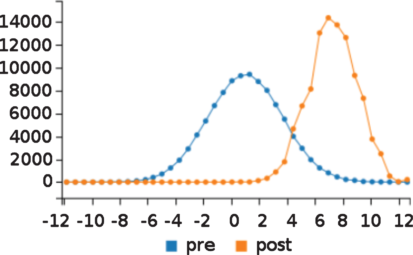
The query $\begin{matrix} ? - mc_s ample_a rg (value (0, Y), 100000, Y, L 0), \\ mc_l w_s ample_a rg (value (0, X), (value (1, 9), \\ value (2, 8)), 1000, X, L), \\ densities (L 0, L, 40, Chart) . \end{matrix}$ takes 100,000 samples of the argument X of value(0,X) before and after the observation of value(1,9),value(2,8) and draws the prior and posterior densities of the samples using a line chart. Figure 9 shows the resulting graph where the posterior is clearly peaked at around 7.

Fig.9

Prior and posterior densities in gauss_mean_est.pl.

5.8 Kalman filter

The example (http://cplint.lamping.unife.it/example/inference/kalman_filter.pl) (adapted from [15]) encodes a Kalman filter, i.e., a Hidden Markov model with a real value as state and a real value as output. $\begin{matrix} kf (N, O, T) : - init (S), kf_p art (0, N, S, O, T) . \\ kf_p art (I, N, S, [V | RO], T) : - I < N, NextI is I + 1, \\ trans (S, I, NextS), emit (NextS, I, V), \\ kf_p art (NextI, N, NextS, RO, T) . \\ kf_p art (N, N, S, [], S) . \\ trans (S, I, NextS) : - NextS = : = E + S, trans_e rr (I, E) . \\ emit (NextS, I, V) : - V = : = NextS + X, obs_e rr (I, X) . \\ init (S) : gaussian (S, 0, 1) . \\ trans_e rr (_, E) : gaussian (E, 0, 2) . \\ obs_e rr (_, E) : gaussian (E, 0, 1) . \end{matrix}$ The next state is given by the current state plus Gaussian noise (with mean 0 and variance 2 in this example) and the output is given by the current state plus Gaussian noise (with mean 0 and variance 1 in this example). A Kalman filter can be considered as modeling a random walk of a single continuous state variable with noisy observations.

Continuous random variables are involved in arithmetic expressions (in the predicates trans/3 and emit/3). It is often convenient, as in this case, to use CLP(R) constraints so that the same clauses can be used both to sample and to evaluate the weight of the sample on the basis of the evidence, otherwise different clauses have to bewritten.

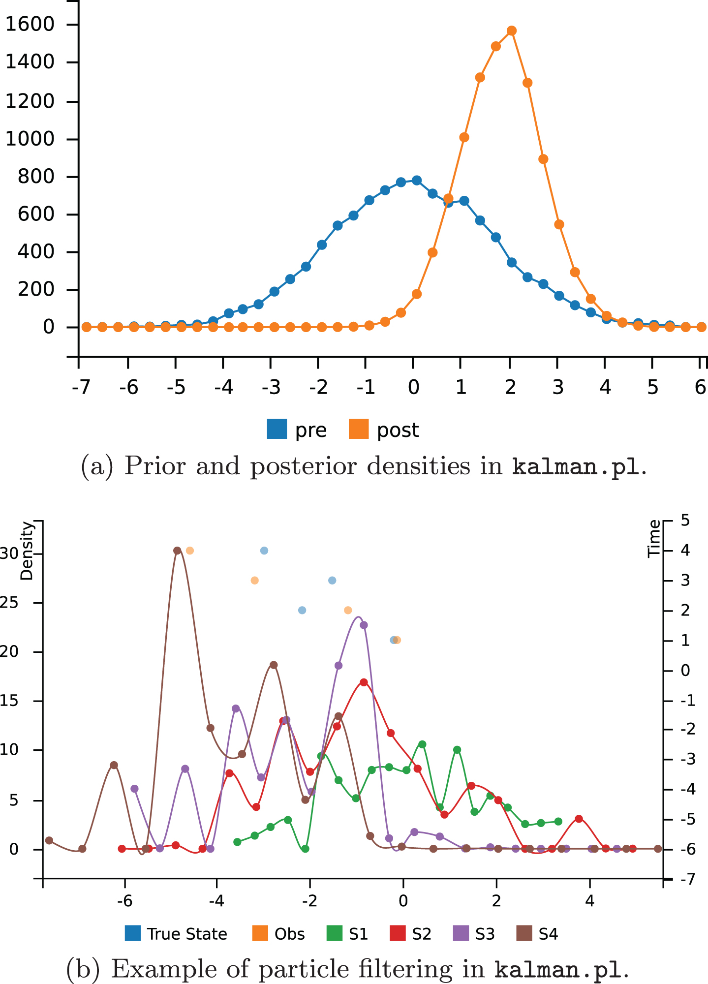
Given that at time 0 the value 2.5 was observed, what is the distribution of the state at time 1 (filtering problem)? Likelihood weighting can be used to condition the distribution on evidence on a continuous random variable (evidence with probability 0). CLP(R) constraints allow both sampling and weighting samples with the same program: when sampling, the constraint V=:=NextS+X is used to compute V from X and NextS. When weighting, the constraint is used to compute X from V and NextS. The above query can be expressed with $\begin{matrix} ? - mc_s ample_a rg (kf (1,_O 1, Y), 10000, Y, L 0), \\ mc_l w_s ample_a rg (kf (1,_O 2, T), kf (1, [2.5],_T), \\ 10000, T, L), \\ densities (L 0, L, 40, Chart) . \end{matrix}$ that returns the graph of Fig. 10a, from which it is evident that the posterior distribution is peaked around 2.5.

Fig.10

Representation of the distributions in the kalman_filter.pl example.

Given a Kalman filter with four observations, the value of the state at the same time points can be sampled by running particle filtering: $\begin{matrix} ? - [O 1, O 2, O 3, O 4] = [- 0.133, - 1.183, - 3.212, - 4.586], \\ mc_p article_s ample_a rg ([kf_f in (1, T 1), kf_f in (2, T 2), \\ kf_f in (3, T 3), kf_f in (4, T 4)], [kf_o (1, O 1), kf_o (2, O 2), \\ kf_o (3, O 3), kf_o (4, O 4)], 100, [T 1, T 2, T 3, T 4], \\ [F 1, F 2, F 3, F 4]) . \end{matrix}$ The list of samples is returned in [F1,F2,F3,F4], with each element being the sample for a time point.

Given the states from which the observations were obtained, Fig. 10bb shows a graph with the distributions of the state variable at time 1, 2, 3 and 4 (S1, S2, S3, S4, density on the left Y axis) and with the points for the observations and the states with respect to time (time on the right Y axis).

5.9 Stochastic logic programs

Stochastic logic programs (SLPs) [13] are a probabilistic formalism where each clause is annotated with a probability. The probabilities of all clauses with the same head predicate sum to one and define a mutually exclusive choice on how to continue a proof. Furthermore, repeated choices are independent, i.e., no stochastic memorization is done. SLPs are used most commonly for defining a distribution over the values of arguments of a query. SLPs are a direct generalization of probabilistic context-free grammars and are particularly suitable for representing them. For example, the grammar

$\begin{matrix} 0.2 : S - > aS 0.2 : S - > bS 0.3 : S - > a 0.3 : S - > b \end{matrix}$ can be represented with the SLP $\begin{matrix} 0.2 : : s ([a | R]) : - s (R) . 0.2 : : s ([b | R]) : - s (R) . \\ 0.3 : : s ([a]) . 0.3 : : s ([b]) . \end{matrix}$ This SLP (http://cplint.lamping.unife.it/example/inference/slp_pcfg.pl) can be encoded in cplint as: $\begin{matrix} s_a s (N) : 0.2; s_b s (N) : 0.2; s_a (N) : 0.3; s_b (N) : 0.3 . \\ s ([a | R], N 0) : - s_a s (N 0), N 1 is N 0 + 1, s (R, N 1) . \\ s ([b | R], N 0) : - s_b s (N 0), N 1 is N 0 + 1, s (R, N 1) . \\ s ([a], N 0) : - s_a (N 0) . s ([b], N 0) : - s_b (N 0) . \\ s (L) : - s (L, 0) . \end{matrix}$ where we have added an argument to s/1 for passing a counter to ensure that different calls to s/2 are associated with independent random variables.

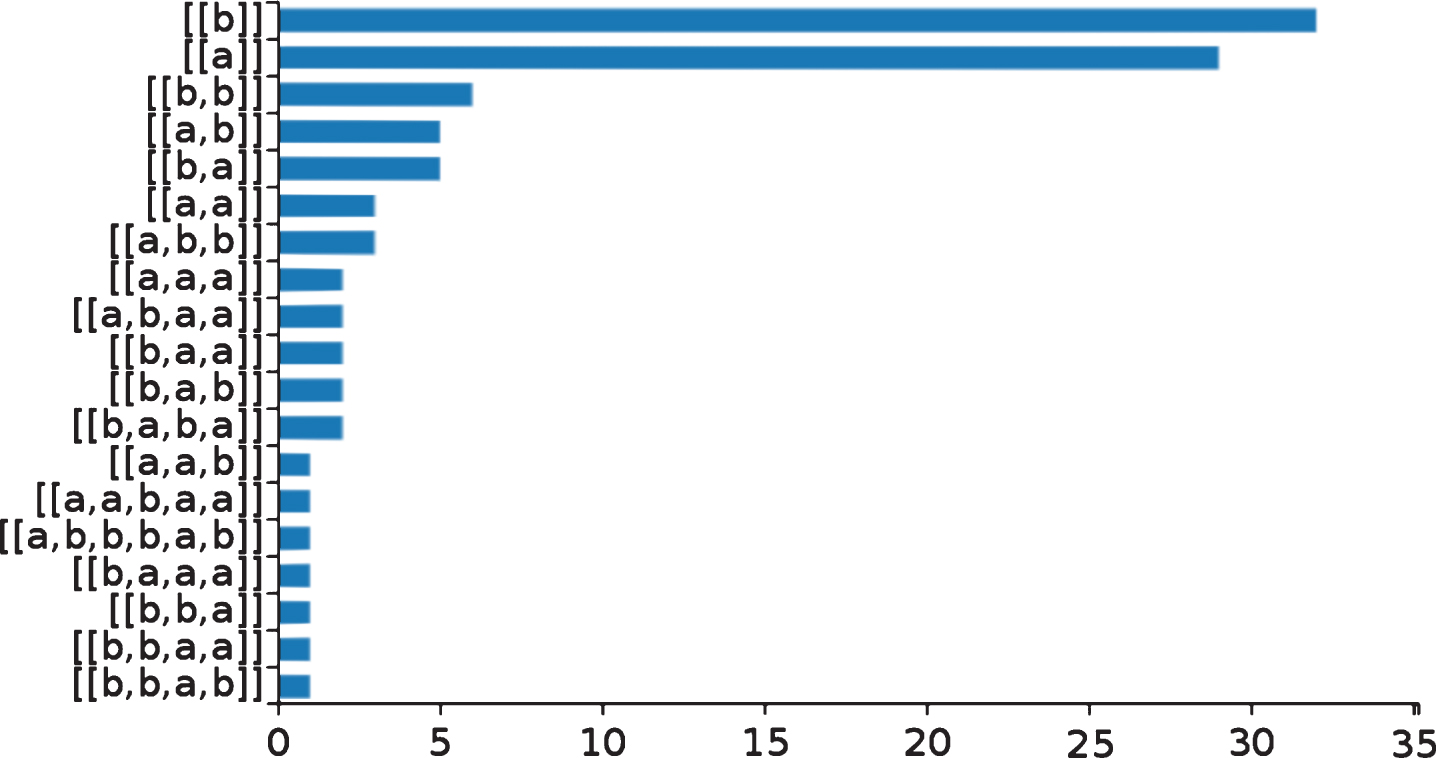
By using the argument sampling features of cplint we can simulate the behavior of SLPs. For example the query $? - mc_s ample_a rg_b ar (s (S), 100, S, L) .$ samples 100 sentences from the language and draws the bar chart of Fig. 11.

Fig.11

Samples of sentences of the language defined in slp_pcfg.pl.

6 Conclusions

cplint on SWISH is a web application for PLP that offers many features, including some that used to be present only in other PP paradigms, such as functional or imperative PP. For example, the possibility of handling hybrid programs, containing both discrete and continuous variables, is relatively novel in PLP and cplint on SWISH is the first online system offering it.

cplint on SWISH allows users to perform reasoning tasks by using just a web browser, without requiring the installation of a PLP system on their machine, an usually complex process. In this way we hope to reach out to a wider audience and increase the user base of PLP.

In the future we plan to explore in more detail the connection with PP using functional/imperative languages and exploit the techniques developed in that field. We are currently working on supporting a probabilistic extension [2] of hybrid logic knowledge bases [12], for combining probabilistic logic programming with probabilistic description logics. Moreover, we plan to add the support to tractable languages and causal probability theory. Finally, we are working on the implementation of a new feature which will allow users to exploit also the R language for improving statistical computingfunctionalities. A complete online tutorial [18] is available at (http://ds.ing.unife.it/~gcota/plptutorial/).

Acknowledgments

This work was supported by the “GNCS-INdAM”.

Footnotes

³http://www.robots.ox.ac.uk/∼fwood/anglican/examples/viewer/?worksheet=gaussian-posteriors

References

Alberti

, Cota

, Riguzzi

and Zese

, Probabilistic logical inference on the web. In Adorni

Giovanni

, Cagnoni

Stefano

, Gori

Marco

and Maratea

Marco

, editors, AI*IA 2016 Advances in Artificial Intelligence, volume 10037 of Lecture Notes in Artificial Intelligence. Springer, 2016.

Alberti

, Lamma

, Riguzzi

and Zese

, Probabilistic hybrid knowledge bases under the distribution semantics. In Adorni

Giovanni

, Cagnoni

Stefano

, Gori

Marco

and Maratea

Marco

, editors, AI*IA 2016 Advances in Artificial Intelligence, volume 10037 of Lecture Notes in Artificial Intelligence, Springer, 2016.

De Raedt

, Kimmig

and Toivonen

, ProbLog: A probabilistic Prolog and its application in link discovery, In Proceedings of the 20th International Joint Conference on Artificial Intelligence, volume 7, pages 2462–2467, Alto, California USA, 2007. AAAI Press.

Darwiche

and Marquis

, A knowledge compilation map, J Artif Intell Res17 (2002), 229–264.

De Raedt

and Kimmig

, Probabilistic (logic) programming concepts, Mach Learn100(1) (2015), 5–47.

Fung

R.M.

and Chang

K.-C.

, Weighing and integrating evidence for stochastic simulation in bayesian networks, In Proceedings of the 5th Annual Conference on Uncertainty in Artificial Intelligence, pages 209–220. North-Holland Publishing Co., 1990.

Fierens

, Van den Broeck

, Renkens

, Sht. Shterionov

, Gutmann

, Thon

, Janssens

and De Raedt

, Inference and learning in probabilistic logic programs using weighted boolean formulas, Theor Pract Log Prog15(3) (2015), 358–401.

Gutmann

, Thon

, Kimmig

, Bruynooghe

and De Raedt

, The magic of logical inference in probabilistic programming, Theor Pract Log Prog11(4-5) (2011), 663–680.

Asiful Islam

, Ramakrishnan

C.R.

and Ramakrishnan

IV.

, Inference in probabilistic logic programs with continuous random variables, Theor Pract Log Prog12 (2012), 505–523.

10.

Kimmig

, Demoen

, De Raedt

, Costa

V.S.

and Rocha

, On the implementation of the probabilistic logic programming language ProbLog, Theor Pract Log Prog11(2-3) (2011), 235–262.

11.

Koller

and Friedman

, Probabilistic Graphical Models: Principles and Techniques. Adaptive computation and machine learning. MIT Press, Cambridge, MA, 2009.

12.

Motik

and Rosati

, Reconciling description logics and rules, J ACM57(5) (2010), 30:1–30:62.

13.

Muggleton

, Learning stochastic logic programs, Electron Trans Artif Intell4(B) (2000), 141–153.

14.

Nitti

, De Laet

and De Raedt

, Probabilistic logic programming for hybrid relational domains, Mach Learn103(3) (2016), 407–449.

15.

Nampally

and Ramakrishnan

C.R.

, Adaptive MCMC-based inference in probabilistic logic programs, arXiv preprint arXiv:1403.6036, 2014.

16.

Pfeffer

, Practical Probabilistic Programming. Manning Publications, 2016.

17.

Riguzzi

, Bellodi

, Lamma

, Zese

and Cota

, Probabilistic logic programming on the web, Software Pract and Exper46(10) (2016), 1381–1396.

18.

Riguzzi

and Cota

, Probabilistic logic programming tutorial, The Association for Logic Programming Newsletter29(1) (2016), 1–1.

19.

Richardson

and Domingos

, Markov logic networks, Mach Learn62(1-2) (2006), 107–136.

20.

Riguzzi

, MCINTYRE: A Monte Carlo system for probabilistic logic programming, Fund Inform124(4) (2013), 521–541.

21.

Riguzzi

, The distribution semantics for normal programs with function symbols, Int J Approx Reason77 (2016), 1–19.

22.

Riguzzi

and Swift

, The PITA system: Tabling and answer subsumption for reasoning under uncertainty, Theor Pract Log Prog11(4-5) (2011), 433–449.

23.

Sato

, A statistical learning method for logic programs with distribution semantics. In Sterling

Leon

, editor, Logic Programming, Proceedings of the 12th International Conference on Logic Programming, June 13-16, 1995, Tokyo, Japan, pages 715–729, Cambridge, Massachusetts, 1995. MIT Press.

24.

Von Neumann

, Various techniques used in connection with random digits, Nat Bureau Stand Appl Math Ser12 (1951), 36–38.

25.

Vennekens

, Verbaeten

and Bruynooghe

, Logic Programs With Annotated Disjunctions. Logic Programming: 20th International Conference, ICLP 2004, Saint-Malo, France, September 6-10, 2004. Proceedings, In Demoen

Bart

and Lifschitz

Vladimir

, editors, volume 3132of LNCS, pages 431–445, Berlin Heidelberg, Germany, 2004, Springer Berlin Heidelberg.

26.

Wood

, Willem van de Meent

and Mansinghka

, A new approach to probabilistic programming inference. In, Proceedings of the 17th International conference on Artificial Intelligence and Statistics (2014), 1024–1032.