On the use of the policy gradient and Hessian in inverse reinforcement learning

Abstract

Reinforcement Learning (RL) is an effective approach to solve sequential decision making problems when the environment is equipped with a reward function to evaluate the agent’s actions. However, there are several domains in which a reward function is not available and difficult to estimate. When samples of expert agents are available, Inverse Reinforcement Learning (IRL) allows recovering a reward function that explains the demonstrated behavior. Most of the classic IRL methods, in addition to expert’s demonstrations, require sampling the environment to evaluate each reward function, that, in turn, is built starting from a set of engineered features. This paper is about a novel model-free IRL approach that does not require to specify a function space where to search for the expert’s reward function. Leveraging on the fact that the policy gradient needs to be zero for an optimal policy, the algorithm generates an approximation space for the reward function, in which a reward is singled out employing a second-order criterion. After introducing our approach for finite domains, we extend it to continuous ones. The empirical results, on both finite and continuous domains, show that the reward function recovered by our algorithm allows learning policies that outperform those obtained with the true reward function, in terms of learning speed.

Keywords

Reinforcement learning inverse reinforcement learning policy gradient feature extraction

1 Introduction

Reinforcement Learning (RL) [49] assumes that the implicit notion of “task” (or goal) is encoded in a Markov Decision Process (MDP) [46] by means of the reward function. Provided that the environment is equipped with a reward function, RL offers a wide range of algorithms to estimate an optimal policy, when the dynamics of the environment is unknown [49]. However, there are several real-world cases in which manually devising a reward function is a challenging problem. The classic motivating example, proposed by Abbeel and Ng in [1], is the car driving problem. Specifying a suitable reward function means, in this case, formalizing the intuitive notion of “driving well”. Driving is a complex multi-objective task: a good driver trades off many conflicting desiderata, such as keeping a reasonable speed, staying far from any pedestrian, maintaining a safe following distance. The authors claim that, rather than specifying a reward function, it is easier to generate demonstrations of good drivers, inducing the agent to learn by observation. Learning from expert’s demonstrations is called Apprenticeship Learning (AL), also named learning by watching, imitation learning, or learning from demonstration.

The main approaches for solving this problem are Behavioral Cloning (BC) [2] and Inverse Reinforcement Learning (IRL) [39]. The former recovers the demonstrated policy by learning the state-action mapping in a supervised learning way, while inverse reinforcement learning aims to learn a reward function that makes the expert optimal. Behavioral cloning is simple, but its main limitation is the intrinsic goal, i.e., to replicate the observed policy. This has several drawbacks: it requires a huge amount of data when the environment (or the expert) is stochastic [22]; it does not provide good generalization or a description of the expert’s goal. On the contrary, inverse reinforcement learning accounts for generalization and transferability by directly learning a reward function. This information can be transferred to any new environment; as a consequence, IRL allows recovering an optimal policy a posteriori, even under variations of the environment. Furthermore, the expert’s policy might be very far from the class of policies that the learner can play (e.g., a human demonstrator and a robotic learner). Therefore, the best policy recovered by behavioral cloning could display worse performance w.r.t. a policy learned by optimizing a reward function of the problem. IRL has received a lot of attention in the literature and has succeeded in several applications [e.g., 1, 17, 23, 48, 52, 62].

It is important to stress that the reward function is more powerful and compact information w.r.t. the optimal policy. The transition model can change over time, due to external factors, as a consequence also the optimal policy might change. However, the reward encodes the notion of “task” and thus, it will remain the same. Knowing the reward, we can recompute an optimal policy associated with the new MDP. Nevertheless, BC and IRL are tightly related by the intrinsic relationship between reward and optimal policy. The reward function defines the space of optimal policies and to recover a reward it is required to observe/recover an optimal policy. However, also IRL approaches pose some relevant challenges. First, several IRL methods require solving the forward RL problem as part of an inner loop in order to evaluate the quality of each candidate reward [e.g., 1, 52]. Literature has extensively focused on removing this limitation [28, 44, 45] in order to scale IRL to real-world applications [16, 21, 22]. Second, IRL methods generally require designing the function space by providing features that capture the structure of the reward function [e.g., 1, 3, 28, 45, 47, 52, 54]. This information, provided in addition to expert’s demonstrations, is critical for the success of the IRL approach. The issue of designing the function space is a well-known problem in supervised learning, but it is even more critical in IRL since a wrong choice might prevent from finding good solutions to the IRL problem [37, 39], especially when linear reward models are considered. The importance of incorporating feature construction in IRL has been known in the literature for a while [1], but, as far as we know, it has been explicitly addressed only in [29]. Recently, IRL literature, by mimicking supervised learning one, has focused on exploiting the neural network capability of automatically constructing relevant features out of the provided data [e.g., 16, 21, 23]. By exploiting a “black-box” approach, these methods do not take advantage of the structure of the underlying Markov decision process (in the phase of feature construction).

In this paper, we revise Compatible Reward Inverse Reinforcement Learning (CR-IRL), an algorithm that constructs reward features directly from expert’s demonstrations. CR-IRL is model-free and does not require solving the forward problem (i.e., finding an optimal policy given a candidate reward function) as an inner step. The algorithm builds a reward function that is compatible with the expert’s policy. It mixes BC and IRL in order to recover the “optimal” and most “informative” reward function in the space spanned by the recovered features. Inspired by the gradient-minimization IRL approach proposed in [45], we focus on the space of reward functions that makes the policy gradient of the expert vanish. Since a zero gradient is only a necessary condition for optimality, we consider a second order optimality criterion based on the policy Hessian to rank the reward functions and finally select the best one (i.e., the one that penalizes the most a deviation from the expert’s policy). This work is an extension of [36] and the main contributions are: i) a deeper analysis of the problem of estimating the expert’s policy (Section 4); ii) a more detailed discussion of the second-order criteria for recovering the reward function, including a multi-objective view of the problem (Section 6); iii) a theoretical analysis of the algorithm, including a computational complexity analysis and a finite-sample analysis of the feature extraction phase (Section 7); iv) a wider experimental campaign including new experiments and a new domain (Section 9).

2 Preliminaries

A Markov Decision Process (MDP) [46] is defined as a tuple $M = (S, A, P, R, μ, γ)$ , where $S$ is the state space, $A$ is the action space, P is a Markovian transition model that, given a state s and an action a, defines a probability distribution over the next state P (· |s, a), R is the reward function, that given a state s and an action a assigns R (s, a), the reward the agent gets by performing action a in state s, μ is the probability distribution of the initial state and γ ∈ [0, 1] is the discount factor. The behavior of an agent is specified by a Markovian policy π, that given a state s, defines a probability distribution over the actions π (· |s). The goal of a reinforcement learning agent is to find an optimal policy, i.e., a policy π^* that maximizes the expected return $J_{μ}^{π}$ , defined as the expected discounted sum of the rewards the agent collects: $J_{μ}^{π} = \underset{s_{0} \sim μ a_{t} \sim π (\cdot | s_{t}) s_{t + 1} \sim P (\cdot | s_{t}, a_{t})}{E} [\sum_{t = 0}^{+ \infty} γ^{t} R (s_{t}, a_{t})] .$ (1)

We consider the case in which the policy belongs to a parametric policy space Π_Θ = {π_θ : θ ∈ Θ ⊆ IR^k} and we denote with J (θ) the quantity $J_{μ}^{π_{θ}}$ . Therefore, finding the optimal policy translates into finding the best parametrization θ^*: $θ^{*} \in \underset{θ \in Θ}{\arg \max} J (θ) .$ (2)

We now discuss how the expected return can be actually computed, introducing the trajectory view and the state-action view.

2.1 Trajectory view

Consider a policy π_θ and suppose to run π_θ for H ∈ IN ∪ {+ ∞} time steps in the environment. 1 In this process, we will encounter a sequence of states and actions, namely a trajectory. We will denote with $τ = (s_{τ, 0}, a_{τ, 0}, s_{τ, 1}, a_{τ, 1}, \dots, s_{τ, H - 1}, a_{τ, H - 1}, s_{τ, H}) \in T$ a trajectory of length H, with $T$ the set of all trajectories and with p_θ (τ) the probability density function of a trajectory τ, defined as: $p_{θ} (τ) = μ (s_{τ, 0}) \prod_{t = 0}^{H - 1} π_{θ} (a_{τ, t} | s_{τ, t}) P (s_{τ, t + 1} | s_{τ, t}, a_{τ, t}) .$ (3) Using this quantity, we can express the expected return as an expectation in the trajectory space $T$ [43]: $J (θ) = E_{τ \sim p_{θ}} [R (τ)],$ (4) where $R (τ) = \sum_{t = 0}^{H - 1} γ^{t} R (s_{τ, t}, a_{τ, t})$ is the return of trajectory τ.

2.2 State-action view

A policy π_θ, combined with the transition model P and the distribution of the initial state μ, generates a visiting distribution of the states of the MDP. We define the γ-discounted state distribution $d_{μ}^{π_{θ}}$ [51] as the normalized discounted number of times a state s is visited following policy π_θ for H time steps: $\begin{matrix} d_{μ}^{π_{θ}} (s) = \frac{1 - γ}{1 - γ^{H}} \sum_{t = 0}^{H - 1} γ^{t} Pr (s_{t} = s | π_{θ}) . \end{matrix}$ Similarly, we can define the γ-discounted state-action distribution as $d_{μ}^{π_{θ}} (s, a) = d_{μ}^{π_{θ}} (s) π_{θ} (a | s)$ , that represents the normalized discounted number of times action a is taken in state s following policy π_θ for H timesteps. Using these distributions, we can redefine the expected return as an expectation taken under $d_{μ}^{π_{θ}}$ [51]: $J (θ) = \frac{1}{1 - γ} E_{(s, a) \sim d_{μ}^{π_{θ}}} [R (s, a)] .$ (5)

Furthermore, when we are not interested in the initial state distribution μ, we can define the state value function [49] as the expected return obtained by starting in state s and following policy π_θ thereafter (Bellman equation): $V^{π_{θ}} (s) = E_{a \sim π_{θ} (\cdot | s) s^{'} \sim P (\cdot | s, a)} [R (s, a) + γ V^{π_{θ}} (s^{'})] .$ (6) For control purposes, the state-action value function, or Q-function [49], is introduced as the expected return starting from a state s, performing action a and then following policy π_θ (Bellman equation): $Q^{π_{θ}} (s, a) = R (s, a) + γ E_{s^{'} \sim P (\cdot | s, a) a^{'} \sim π_{θ} (\cdot | s^{'})} [Q^{π_{θ}} (s^{'}, a^{'})] .$ (7) These functions are tightly connected due to the trivial relation: $V^{π_{θ}} (s) = E_{a \sim π_{θ} (\cdot | s)} [Q^{π_{θ}} (s, a)]$ . Finally, we define the advantage function [4]: $A^{π_{θ}} (s, a) = Q^{π_{θ}} (s, a) - V^{π_{θ}} (s),$ (8) that quantifies how much playing action a is better than following policy π_θ in state s.

3 Algorithm overview

In this section, we provide a high-level overview of CR-IRL. CR-IRL takes as input a parametric policy space Π_Θ and a set of trajectories $D = {τ_{i}}_{i = 1}^{N}$ generated by the expert policy π^E. CR-IRL is a non-iterative algorithm that recovers a reward function for which the expert is optimal without requiring to specify a reward function space. It starts building the features ϕ_i of the value function that are compatible with policy π^E, i.e., that make the policy gradient vanish (Phase 1, Section 5). Since π^E might not belong to Π_Θ, this step requires a parametric representation π_{θ

^E} ∈ Π_Θ of the expert’s policy which can be obtained through behavioral cloning (Section 4). 2 The choice of the policy space Π_Θ influences the size of the functional space used by CR-IRL for representing the value function (and the reward function) associated with the expert’s policy. In order to formalize this notion, we introduce the policy rank, a quantity that represents the ability of a parametric policy to reduce the dimensions of the approximation space for the value function of the expert’s policy (Section 5.1). Once these value features have been built, they can be transformed into reward features ψ_i (Phase 2, Section 5.2) by means of the Bellman equation [46] (model-based) or reward shaping [38] (model-free). All the rewards spanned by the features ψ_i satisfy the first-order necessary optimality condition [40], but we are not sure about their nature (minima, maxima or saddle points). The final step is thus to recover a reward function that is maximized by the expert’s policy (Phase 3, Section 6). This is achieved by considering a second-order optimality condition, with the idea that we want the reward function that penalizes the most a deviation from the parameters of the expert’s policy π_{θ

^E}. This criterion is similar in spirit to what done in [1, 39, 47], where the goal is to identify the reward function that makes the expert’s policy better than any other policy by a margin.

IRL literature usually considers two different settings: optimal or sub-optimal expert. This distinction is necessary when a fixed reward space is provided, knowing that an optimal expert would maximize a reward within that space. If the demonstrated behavior happens to be suboptimal, then the IRL problem becomes somehow not well defined and might result infeasible, as the reward actually optimized by the (suboptimal) expert might fall outside the considered space. In this case, additional “optimality” criteria are required [37]. This is not the case for CR-IRL that is able to automatically generate the space of reward functions that make the policy gradient vanish. In this way, the space would contain also reward functions under which the recovered expert’s policy π_{θ

^E} is optimal, no matter if the expert is suboptimal w.r.t. to some unknown reward.

4 Estimating the expert’s policy

Approximating the expert’s policy π^E can be formulated as a probability estimation problem, solved by exploiting the available expert’s trajectories ${τ_{i}}_{i = 1}^{N}$ , generated by policy π^E. Informally, given a class of parametric policies Π_Θ we aim to find the policy that best represents the unknown expert’s policy π^E. For this purpose, we employ the classical Maximum Likelihood (ML) [12] and Maximum A Posteriori (MAP) [5] approaches. In the former case, we look for the parameters θ^ML that maximize the likelihood function: $L (θ) = p ({τ_{i}}_{i = 1}^{N} | θ) = \prod_{i = 1}^{N} p_{θ} (τ_{i}),$ (9) where p_θ is the trajectory density function induced by the parametrization θ. It can be proved (see Appendix B of [35]) that maximizing equation (9) is equivalent to performing a moment projection of the expert’s policy π^E onto the space Π_Θ. If some knowledge on the expert’s parameters is available we can take advantage of a Bayesian approach. Let p (θ) be a prior distribution over the policy parameters θ, the Maximum A Posteriori (MAP) estimation aims at maximizing the parameter posterior probability: $\begin{matrix} p (θ | {τ_{i}}_{i = 1}^{N}) & = \frac{p ({τ_{i}}_{i = 1}^{N} | θ) p (θ)}{p ({τ_{i}}_{i = 1}^{N})} \\ \propto p ({τ_{i}}_{i = 1}^{N} | θ) p (θ), \end{matrix}$ where $L (θ) = p ({τ_{i}}_{i = 1}^{N} | θ)$ is again the likelihood function. Clearly, when considering an uninformative prior (i.e., p (θ) ∝1) the MAP approach reduces to the ML case.

In the following, we will consider only the ML approach. It is well known that rather than optimizing the likelihood function $L (θ)$ it is more convenient to optimize its logarithm. In our case, starting from equation (3) and observing that the transition model P and the distribution of the initial state μ do not depend on θ, the optimization problem becomes: $θ^{ML} \in \underset{θ \in Θ}{\arg \max} \sum_{i = 1}^{N} \sum_{t = 0}^{H - 1} log π_{θ} (a_{τ_{i}, t} | s_{τ_{i}, t}),$ (10) where each action a_{τ_i,t} is an expect choice, i.e., a_{τ_i,t} ∼ π^E (· |s_{τ_i,t}). Clearly, the selection of the parametric policy space has an impact at least for what concerns the ability to represent the expert’s policy. It is important to point out that policy π_{θ
^ML} will not be used to collect samples, as we assume to have access to the provided trajectories only (batch settings), but just to extract the features for the reward function, as explained in the following sections. Therefore, even an imperfect choice of the policy space has a limited effect on the performance of the algorithm. Nevertheless, a highly inaccurate choice of the policy space might produce a non-optimal approximation space, compromising the effectiveness of the algorithm.

It is worth noting that the ML policy π_{θ
^ML}, even if we have infinite samples, is not necessarily the optimal policy π_{θ
^*} in the policy space Π_Θ, i.e., the policy that maximizes the expected return, as defined in equation (2). When the policy space Π_Θ is sufficiently expressive to contain the expert’s policy, i.e., there exists θ^E ∈ Θ such that π^E = π_{θ
^E}, ML policy converges almost surely to the expert’s policy. On the contrary, when the expert’s policy falls outside Π_Θ, π_{θ
^ML} converges the moment projection of π^E onto Π_Θ [11]: $\underset{θ \in Θ}{\arg \min} E_{τ \sim p^{E}} [\sum_{t = 0}^{H - 1} D_{KL} (π^{E} (\cdot | s_{τ, t}) | π_{θ} (\cdot | s_{τ, t}))],$ where p^E is the probability density function over trajectories induced by the expert’s policy π^E. For brevity, in the followings, we will indicate with π_θ the parametric representation of the expert’s policy.

5 Feature extraction via first-order criterion

In this section, we present the procedure to obtain the set ${ϕ_{i}}_{i = 1}^{p}$ of Expert’s COmpatible Q-features (ECO-Q) that make the policy gradient vanish. 3 We start introducing the policy gradient and the associated first-order optimality condition. Given a stochastic policy π_θ differentiable w.r.t. the parameter θ, the gradient of the expected reward (policy gradient) can be expressed in the trajectory view as [59]: $\nabla_{θ} J (θ) = E_{τ \sim p_{θ}} [\nabla_{θ} log p_{θ} (τ) R (τ)],$ (11) where $\nabla_{θ} log p_{θ} (τ) = \sum_{t = 0}^{H - 1} \nabla_{θ} log π_{θ} (a_{τ, t} | s_{τ, t})$ . In the state-action view the policy gradient becomes [50]: $\nabla_{θ} J (θ) = E_{(s, a) \sim d_{μ}^{π_{θ}}} [\nabla_{θ} log π_{θ} (a | s) Q^{π_{θ}} (s, a)] .$ (12) When π_{θ
^*} is an optimal policy in the class of policies Π_Θ then θ^* is a stationary point of the expected return and thus ∇_θJ (θ^*) = 0 (first-order necessary conditions for optimality [40]).

We assume the space $S \times A$ is a Hilbert space [9] equipped with the weighted inner product: 4

$\begin{matrix} 〈 f, g 〉_{μ, π_{θ}} = E_{(s, a) \sim d_{μ}^{π_{θ}}} [f (s, a) g (s, a)] \\ = \int_{S} \int_{A} f (s, a) d_{μ}^{π_{θ}} (s, a) g (s, a) d s d a . \end{matrix}$ (13) When π_θ is optimal for the MDP, ∇_θ log π_θ and Q^{π
_θ} are orthogonal w.r.t. the inner product (13). We can exploit the orthogonality property to build an approximation space for the Q-function. Let: $G_{π_{θ}} = {\sum_{i = 1}^{k} α_{i} \nabla_{θ_{i}} log π_{θ} : α_{i} \in IR, i = 1, 2, . . ., k}$ be the subspace spanned by the gradient of the log-policy π_θ. From equation (12) finding an approximation space for the Q-function is equivalent to finding the orthogonal complement of the subspace G_{π
_θ}, which in turn corresponds to finding the null space of the functional: $G_{π_{θ}} [ϕ] = 〈 \nabla_{θ} log π_{θ}, ϕ 〉_{μ, π_{θ}} .$ (14) We define an Expert’s COmpatible Q-feature as any function ϕ making the functional (14) null. This space $G_{π_{θ}}^{⊥} = null (G_{π_{θ}})$ represents the Hilbert subspace of the features for the Q-function that are compatible with the policy π_θ in the sense that any Q-function optimized by policy π_θ can be expressed as a linear combination of those features. Sections 5.2.1 and 5.2.2 describe how to compute the ECO-Q from samples in finite and continuous MDPs, respectively. The dimension of $G_{π_{θ}}^{⊥}$ is typically very large since the number k of policy parameters is significantly smaller than the number of state-action pairs. A formal discussion of this issue for finite MDPs is presented in the next section.

5.1 Policy rank

The parametrization of the expert’s policy influences the size of $G_{π_{θ}}^{⊥}$ . Intuition suggests that the larger the number k of the parameters the more the policy is informative to infer the Q-function and so the reward function. This is motivated by the following rationale. Consider representing the expert’s policy using two different policy models such that one model is a superclass of the other one (for instance, assume to use linear models where the features used in the simpler model are a subset of the features used in the other model). All the reward functions that make the policy gradient vanish with the rich policy model, do the same with the simpler model, while the vice versa does not hold. This suggests that complex policy models are able to reduce more the space of optimal reward function w.r.t. simpler models. This notion plays an important role for finite MDPs, i.e., MDPs where the state-action space is finite. We formalize the ability of a policy to infer the characteristics of the MDP with the concept of policy rank.

Definition 5.1. Let π_θ a policy with k parameters belonging to the class Π_Θ and differentiable in θ. The policy rank is the dimension of the space of the linear combinations of the partial derivatives of π_θ w.r.t. θ: $rank (π_{θ}) = dim (Γ_{π_{θ}}),$ where $Γ_{π_{θ}} = {\sum_{i = 1}^{k} α_{i} \nabla_{θ_{i}} π_{θ} : α_{i} \in IR, i = 1, 2, . . ., k} .$

A first important note is that the policy rank depends not only on the policy model Π_Θ, but also on the value of the parameters of the policy π_θ. So the policy rank is a property of the policy not of the policy model. The following bound on the policy rank holds for finite MDPs.

Theorem 5.1. Given a finite MDP $M$ , let π_θ a policy with k parameters belonging to the class Π_Θ and differentiable in θ, then: $rank (π_{θ}) \leq min {k, | S | | A | - | S |},$ where $| X |$ indicates the cardinality of the set $X$ .

Proof. Γ_{π
_θ} is a subspace of ${IR}^{| S | | A |}$ generated by k vectors, thus its dimension cannot be larger than k. For each state $s \in S$ it holds that π_θ (· |s) is a probability density function thus: $\sum_{a \in A} π_{θ} (a | s) = 1, \forall s \in S .$ For all parameters θ_j, j = 1, . . . , k the partial derivatives of the previous equation result in: $\sum_{a \in A} \frac{\partial π_{θ}}{\partial θ_{j}} (a | s) = 0, \forall s \in S, j = 1, 2, . . ., k .$ Let us consider h ∈ Γ_{π
_θ}, by definition of Γ_{π
_θ}, it can be written as a linear combination of the partial derivatives of π_θ: $h = \sum_{j = 1}^{k} α_{j} \frac{\partial π_{θ}}{\partial θ_{j}},$ so for all the states s we have: $\sum_{a \in A} h (a | s) = 0, \forall s \in S .$ These are $| S |$ linearly independent equations, thus the dimension of Γ_{π
_θ} cannot be larger then $| S | | A | - | S |$ .□

From an intuitive point of view this is justified by the fact that π_θ (· |s) is a probability distribution. As a consequence, for all $s \in S$ the probabilities π_θ (a|s) must sum up to one, removing $| S |$ degrees of freedom. This has a relevant impact on the algorithm since it induces a lower bound on the dimension of the orthogonal complement $\dim (G_{π_{θ}}^{⊥}) \geq max {| S | | A | - k, | S |}$ , thus even the most flexible policy (i.e., a policy model with a parameter for each state-action pair) cannot determine a unique reward function that makes the expert’s policy optimal, leaving $| S |$ degrees of freedom. It follows that it makes no sense to consider a policy with more than $| S | | A | - | S |$ parameters. In this sense, the policy rank can be interpreted as the number of effective parameters of the policy.

The bound on the policy rank does not assume any information about the optimality of the policy within the class Π_Θ. Γ_{π
_θ} might lose further dimensions when π_θ is obtained as the maximum likelihood policy from the set of expert’s trajectories.

5.2. Expert’s compatible Q-features

In this section, we discuss how to construct the features for representing the optimal Q-function, for both finite and continuous MDPs.

5.2.1. Construction of ECO-Q in finite MDPs

We now develop in details the algorithm to generate ECO-Q in the case of finite MDPs. From now on we will indicate with $D$ the set of state-action pairs visited by the expert along the available trajectories, i.e., $D = {(s_{τ_{i}, t}, a_{τ_{i}, t})}_{i = 1, . . ., N, t = 0, . . ., H - 1}$ . When the state-action space is finite the inner product (13) can be written in matrix notation as: $〈 f, g 〉_{μ, π_{θ}} = f^{T} D_{μ}^{π_{θ}} g,$ where f, g and $d_{μ}^{π_{θ}}$ are real vectors with $| D |$ components and $D_{μ}^{π_{θ}} = diag (d_{μ}^{π_{θ}})$ . The term ∇_θ log π_θ is a $| D | \times k$ real matrix, thus finding the null space of the functional (14) is equivalent to finding the null space of the matrix $\nabla_{θ} log π_{θ}^{T} D_{μ}^{π_{θ}}$ . This can be done for instance through SVD which allows obtaining a set of orthogonal basis functions Φ. Given that the weight vector $d_{μ}^{π_{θ}} (s, a)$ is usually unknown, it needs to be estimated. A simple Monte Carlo estimate exploiting the expert’s demonstrations in $D$ of length H is:

${\hat{d}}_{μ}^{π_{θ}} (s, a) = \frac{1 - γ}{N (1 - γ^{H})} \sum_{i = 1}^{N} \sum_{t = 0}^{H - 1} γ^{t} 1 ((s_{τ_{i}, t}, a_{τ_{i}, t}) = (s, a)) .$ (15) Alternatively, if we use the estimated policy π_θ as if it were the expert policy and recalling that $d_{μ,}^{π_{θ}} (s, a) = d_{μ}^{π_{θ}} (s) π_{θ} (a | s)$ , we need to estimate just $d_{μ}^{π_{θ}} (s)$ : ${\hat{d}}_{μ}^{π_{θ}} (s) = \frac{1 - γ}{N (1 - γ^{H})} \sum_{i = 1}^{N} \sum_{t = 0}^{H - 1} γ^{t} 1 (s_{τ_{i}, t} = s) .$ (16) Clearly, the quality of these estimators is incomparable from a theoretical standpoint (see Lemma 7.3). This is due to the fact that (15) performs a sample mean over the state-action space, whereas (16) performs a sample mean over the state space only and uses an approximate policy (the one obtained from behavioral cloning) to compute (an exact) expectation over the action space.

5.2.2. Construction of ECO-Q in continuous MDPs

To extend the previous approach to the continuous domain we assume that the state-action space is equipped with the Euclidean distance. Now we can adopt an approach similar to the one exploited to extend Proto-Value Functions (PVF) [30,31] to infinite observation spaces [32]. The problem is treated as a discrete one considering only the state-action pairs visited along the collected trajectories. A Nyström interpolation method is used to approximate the value of a feature in a non-visited state-action pair as a weighted mean of the values of the closest k features. The weight of each feature is computed by means of a Gaussian kernel placed over the Euclidean space $S \times A$ : $\begin{matrix} K ((s, a), (s^{'}, a^{'})) & = \exp (- \frac{1}{2 σ_{S}^{2}} | s - s^{'} |_{2}^{2} - \frac{1}{2 σ_{A}^{2}} | a - a^{'} |_{2}^{2}), \end{matrix}$ where $σ_{S}$ and $σ_{A}$ are respectively the state and action bandwidth. In our setting this approach is fully equivalent to a kernel k-Nearest Neighbors regression: $ϕ (s, a) = \frac{\sum_{(s^{'}, a^{'}) \in D_{(s, a)}^{k}} K ((s, a), (s^{'}, a^{'})) ϕ (s^{'}, a^{'})}{\sum_{(s^{'}, a^{'}) \in D_{(s, a)}^{k}} K ((s, a), (s^{'}, a^{'}))},$ where $D_{(s, a)}^{k}$ is the set of the k closest state-action pairs according to the Euclidean distance and given samples in the dataset $D$ . The main difference with the PVF extension is that we need to interpolate over the state-action space (not only over the state space) since we aim to recover a state-action reward function.

5.3. Expert’s compatible reward features

The set of ECO-Q basis functions allows representing the optimal value function under the policy π_θ. In this section, we will show how it is possible to exploit ECO-Q functions to generate basis functions for the reward representation.

We propose two approaches: the first is based on explicit application of Bellman equation and requires the knowledge of the transition model; the second is model-free and exploits optimality-invariant reward transformations. The obtained features, named Expert’s COmpatible Reward features (ECO-R), still satisfy the first-order optimality condition.

5.3.1. Model-based construction of reward features

The relation between the reward and theQ-function is given by the Bellman Equation (7). Considering only the state-action pairs visited along the available expert’s trajectories $D$ , we can express the Bellman equation in matrix form: 5 $q^{π_{θ}} = r + γ P π_{θ} q^{π_{θ}} .$ (17) Similarly to [28], we can obtain the reward function by reversing the equation r = (I - γPπ_θ) q^{π
_θ}. Thus the set of ECO-R ${ψ_{i}}_{i = 1}^{p}$ are obtained by means of the linear mapping of the ECO-Q ${ϕ_{i}}_{i = 1}^{p}$ : $Ψ = (I - γ P π_{θ}) Φ .$ (18) This transformation, however, requires the knowledge of the transition model P which in most of the real cases cannot be assumed. As shown in [28], in order to exploit only expert’s demonstrations, it is necessary to resort to heuristics that may be hard to compute in practice or to additional samples for exploration of the system dynamics.

5.3.2. Model-free construction of reward features

Reversing the Bellman equation allows finding the reward space that generates the estimated Q-function. However, IRL is interested in finding just a reward space under which the expert’s policy is optimal. This problem can be seen as an instance of reward shaping [38] where the authors show that the space of all the reward functions sharing the same optimal policy is given by: $R^{'} (s, a) = R (s, a) + γ E_{s^{'} \sim P (\cdot | s, a)} [χ (s^{'})] - χ (s),$ where χ (s) is a state-dependent potential function. A smart choice [38] is to set χ = V^{π
_θ} under which the new reward space is given by the advantage function: R′ (s, a) = Q^{π
_θ} (s, a) - V^{π
_θ} (s) = A^{π
_θ} (s, a). Thus the expert’s advantage function is an admissible reward optimized by the expert’s policy itself. This choice is, of course, related to using Q^{π
_θ} as reward. However, the advantage function encodes more local and more transferable information w.r.t. the Q-function. In general, the advantage function can be expressed in matrix form as: $a^{π_{θ}} = q^{π_{θ}} - {\tilde{v}}^{π_{θ}} = (I - {\tilde{π}}_{θ}) q^{π_{θ}},$ (19) where ${\tilde{v}}^{π_{θ}}$ is a $| S | | A |$ -dimensional vector obtained from the $| S |$ -dimensional vector v^{π
_θ} repeating each component $| A |$ times. Analogously ${\tilde{π}}_{θ}$ is a $| S | | A | \times | S | | A |$ matrix obtained from the $| S | \times | S | | A |$ matrix π _θ repeating each row $| A |$ times. This holds for the full state-action space. When the expert visited a limited number of state-action pairs, the transformation requires repeating only the rows of the matrix π _θ associated to visited states for a number of times equal to the number of distinct actions performed by the expert in that state. Thus, the space of reward features can be recovered through matrix equality: $Ψ = (I - {\tilde{π}}_{θ}) Φ .$ (20) Notice that this is a simple linear transformation through the expert’s policy. However, the transformation does not preserve the orthogonality of features Φ, thus it is necessary to apply SVD again to get an orthogonal basis of the recovered approximation space. Furthermore, since $I - {\tilde{π}}_{θ}$ is not full-rank, the recovered space has a smaller dimensionality. The specific choice of the state-potential function has the advantage to improve the learning capabilities of any RL algorithm [38]. This is not the only choice of the potential function possible, but it enables model-free estimation.

In the next section, we propose a new method to single out a unique reward function, based on the optimization of a second-order criterion that favors reward functions that significantly penalize deviations from the expert’s policy. Once the ECO-R basis functions have been generated, they can be used, in principle, to feed any IRL algorithm that represents the expert’s reward through a linear combination of basis functions. We will show empirically, that the best performances are obtained when coping our feature construction with the reward selection presented below.

6 Reward selection via second-order criterion

Any linear combination of the ECO-R ${ψ_{i}}_{i = 1}^{p}$ makes the gradient vanish, however in general this is not sufficient to ensure that the policy parameter θ is a maximum of J (θ). Combinations that lead to minima or saddle points should be discarded. Furthermore, provided that a subset of ECO-R leading to maxima has been selected, we should identify a single reward function in the space spanned by this subset of features. Both these requirements can be enforced by imposing a second-order optimality criterion based on the policy Hessian that is given by [18, 25]: $\begin{matrix} H_{θ} J (θ, ω) & = E_{τ \sim p_{θ}} [(\nabla_{θ} log p_{θ} (τ) \nabla_{θ} log {p_{θ} (τ)}^{T} \\ + H_{θ} log p_{θ} (τ)) R (τ, ω)], \end{matrix}$ where ω is the reward weight and the reward is obtained as a linear combination of the ECO-Rs: $R (τ, ω) = \sum_{i = 1}^{p} ω_{i} \sum_{t = 0}^{H - 1} γ^{t} ψ_{i} (s_{τ, t}, a_{τ, t}) .$ (21) It is worth to point out that the linear parametrization, in this case, does not represent a limitation of the algorithm. Indeed, we defined the approximation space of the reward function as the Hilbert space whose functions make the policy gradient vanish. This space will contain all the reward functions optimized by the expert’s policy and each function in that space can be expressed as a linear combination of the elements in a basis, like the ECO-Rs.

6.1 Maximum eigenvalue optimality criterion

To retain only maxima we need to impose that the Hessian is negative definite which is equivalent to require that the maximum eigenvalue $λ_{max} (H_{θ} J (θ, ω))$ is negative. The requirement $λ_{\max} (H_{θ} J (θ, ω)) < 0$ is only a constraint, in order to single out a reward function we need an optimality criterion over the Hessian. We aim to find the reward function that best represents the optimal policy parametrization in the sense that even a slight alteration of the policy parameters induces a dramatic degradation of the performance. Geometrically this corresponds to finding the reward function for which the expected return locally represents the sharpest hyper-paraboloid. Analytically this condition can be enforced by minimizing the maximum eigenvalue of the Hessian whose eigenvector corresponds to the direction of minimum curvature (Maximum Eigenvalue Optimality Criterion, ME-opt). The problem can be formalized using Semi-Definite Programming (SDP): $\begin{array}{l} \underset{ω \in R^{p}}{minimize} λ_{max} (ℋ_{θ} J (θ, ω)) \\ subject to ℋ_{θ} J (θ, ω) + κ I ≼ 0 n \\ ‖ ω ‖_{2} \leq 1, n \end{array}$ where κ ≥ 0 is a threshold to ensure the Hessian is (strictly) negative definite. The constraint |ω|₂ ≤ 1 on the reward parameters is necessary to ensure that the problem is bounded, otherwise, if the problem is feasible, the maximum eigenvalue can be made arbitrarily negative. Clearly, the constraint on the weights will be satisfied with equality, i.e., |ω|₂ = 1, when the problem admits a solution.

In our framework, the reward function can be expressed as a linear combination of the ECO-R so we can rewrite the Hessian as: $H_{θ} J (θ, ω) = \sum_{i = 1}^{p} ω_{i} H_{θ} J_{i} (θ),$ (22) where J_i (θ) is the expected return considering ψ_i as reward function.

Being the Hessian symmetric and defined through an affine function of the variables ω, the maximum eigenvalue is convex [41]. This is a consequence of the fact that we can define $λ_{\max} (H_{θ} J (θ, ω)) = max_{| x |_{2} \leq 1} x^{T} H_{θ} J (θ, ω) x$ , which is the maximum of an affine function in ω over a convex set |x|₂ ≤ 1. Anyway, we can rephrase the problem by removing the λ_max function: $\begin{array}{l} \underset{ω \in R^{p}}{minimize} t \\ subject to ℋ_{θ} J (θ, ω) - t I ≼ 0 \\ t \leq - κ \\ ‖ ω ‖_{2} \leq 1. \end{array}$

This optimization problem is for sure feasible (for sufficiently small κ) since, as already seen, the true reward function and the advantage function make the expert’s policy parametrization optimal. However, in most of the cases, it is impractical to solve, at least for two reasons. First, the computational effort is enormous even for few policy parameters. Second, it might be the case that the strict negative definiteness constraint is never satisfied due to blocked-to-zero eigenvalues. This problem arises quite often and is related to the presence of “useless” policy parameters that even if modified do not affect the policy performance (for instance, a subset of parameters which are linearly dependent). In those cases $λ_{\max} (H_{θ} J (θ, ω))$ would be zero no matter which reward weights ω are selected.

6.2 Trace optimality criterion

In order to account for the possible presence of blocked-to-zero eigenvalues, we need to consider all the eigenvalues of the Hessian matrix instead of the maximum one only. When in the direction of minimum curvature the curve is flat (like in case of blocked-to-zero eigenvalues) we aim to maximize an index of the overall concavity. The trace of the Hessian, being the sum of the eigenvalues, can be used for this purpose. Minimizing the trace of the Hessian (Trace Optimality Criterion, TR-opt) can be formulated in the following semi-definite programming problem: $\begin{array}{l} \underset{ω \in R^{p}}{minimize} tr (ℋ_{θ} J (θ, ω)) \\ subject to ℋ_{θ} J (θ, ω) + κ I ≼ 0 \\ ‖ ω ‖_{2} \leq 1. \end{array}$ (23) The trace is a linear function, i.e., $tr (H_{θ} J (θ, ω)) = \sum_{i = 1}^{p} ω_{i} tr (H_{θ} J_{i} (θ))$ , thus the objective function is for sure convex. Like for the maximum eigenvalue optimality criterion a normalization constraint on the reward parameters is necessary to ensure boundedness. The negative definiteness constraint becomes substantial to ensure the optimality since there might be ECO-Rs with negative trace but positive eigenvalues. Moreover, in presence of blocked-to-zero eigenvalues, κ should be set to zero to ensure feasibility. This formulation, although less demanding w.r.t. the previous one still displays performance degradation as the number of basis functions increases due to the negative definiteness constraint.

6.3 Trace heuristic criterion

Solving the semidefinite programming problem of one of the presented optimality criteria is unfeasible for almost all the real world problems. We are interested in formulating a non-SDP problem, which is a surrogate of the trace optimality criterion, that can be solved more efficiently (Trace Heuristic Criterion, TR-heu). Essentially, we need to get rid of the semi-definiteness constraint.

We assume that the ECO-Rs are orthonormal in order to compare them. 6 The main challenge is how to select the weight ω in order to get a (near-)optimal trace minimizer that preserves the negative semi-definiteness constraint.

Given two symmetric matrices A and B, it holds from Weyl’s inequality that λ_max (A) + λ_max (B) ≤ λ_max (A + B), thus any linear combination of semidefinite matrices with positive coefficients for the negative semidefinite ones and negative coefficients for the positive semidefinite ones is guaranteed to yield a negative semidefinite matrix. In principle, nothing can be ensured for the indefinite matrices, without looking at the magnitude of the eigenvalues. Therefore, we get a feasible solution by retaining only the ECO-Rs yielding a semidefinite Hessian and switching sign to those with positive semidefinite Hessian. Here is a simple example to clarify the procedure.

Example 6.1. Suppose we generated three ECO-Rs ${ψ_{i}}_{i = 1}^{3}$ on a 2-states MDP with two actions with a policy π_θ made of two parameters θ = (θ₁, θ₂) ^T: $ψ_{1} = (\begin{matrix} 1000 \end{matrix}), ψ_{2} = (\begin{matrix} 01 / \sqrt{2} - 1 / \sqrt{2} 0 \end{matrix}), ψ_{3} = (\begin{matrix} 000 - 1 \end{matrix}) .$ We report below the eigenvalues of the Hessian matrices ${H_{θ} J_{i} (θ)}_{i = 1}^{3}$ : $λ_{1} = (\begin{matrix} - 0.1 - 1.2 \end{matrix}), λ_{2} = (\begin{matrix} 3 2.7 \end{matrix}), λ_{3} = (\begin{matrix} 1 - 1.5 \end{matrix}) .$ We discard ψ₃ as it has an indefinite Hessian and we retain ψ₁ and ψ₂. In particular, we switch the sign of ψ₂ so that -ψ₂ has negative eigenvalues. Any combination of the form ω₁ψ₁ - ω₂ψ₂ with ω₁, ω₂ ≥ 0 will induce a negative semidefinite Hessian, thanks to Weyl’s inequality.

Notice that, in this way, we can lose the optimal solution since the trace minimizer might assign a non-zero weight to an ECO-R with indefinite Hessian. For brevity, we will indicate with ${tr}_{i} = tr (H_{θ} J_{i} (θ))$ and tr the vector whose components are tr_i, i = 1, 2, . . . , p. SDP is no longer needed: $\begin{array}{l} \underset{ω \in R^{p}}{minimize} ω^{T} t r \\ subject to ‖ ω ‖_{2} = 1. \end{array}$ (24) The constraint |ω|₂ = 1 ensures that, when the ECO-Rs are orthonormal, the resulting ECO-R has Euclidean norm one. This is a convex programming problem with linear objective function and quadratic constraint, the closed form solution can be found with the Lagrange multipliers.

Theorem 6.1. If all ECO-Rs yield a negative semidefinite Hessian, the solution of the TR-heu problem (24) is given by: $ω_{i} = - \frac{{tr}_{i}}{| tr |_{2}}, i = 1, 2, . . ., p .$ (25)

Proof. We assume to consider a set of ECO-R, yielding negative semidefinite Hessian. The Lagragian function is: $L (ω, α) = \sum_{i = 1}^{p} ω_{i} {tr}_{i} + α (\sum_{i = 1}^{p} ω_{i}^{2} - 1),$ where α is the Lagrange multiplier. We impose that partial derivatives of $L$ w.r.t. ω_j and α vanish, thus: $\begin{array}{l} \frac{\partial ℒ}{\partial ω_{j}} = t r_{j} + 2 α ω_{j} = 0, j = 1, 2, ..., p, \\ \frac{\partial ℒ}{\partial α} = \sum_{i = 1}^{p} ω_{i}^{2} - 1 = 0. \end{array}$ From the first equation, for α ≠ 0, we obtain an expression of ω_j as a function of α: $ω_{j} = - \frac{{tr}_{j}}{2 α}, j = 1, 2, . . ., p .$ The case α = 0 is uninteresting since it is feasible only if all traces are null. By substitution we obtain an expression for α: $α = \pm \frac{1}{2} \sqrt{\sum_{i = 1}^{p} {tr}_{i}^{2}} = \pm \frac{1}{2} | tr |_{2} .$ Since we are looking for a minimum, provided that all traces are non positive, the objective function is minimized for non negative weights: $ω_{j} = - \frac{{tr}_{j}}{\sqrt{\sum_{i = 1}^{p} {tr}_{i}^{2}}} = - \frac{{tr}_{j}}{| tr |_{2}}, j = 1, 2, . . ., p .$ □

6.4. Multi-objective interpretation of the second-order criteria

The intuitive idea behind the second-order criteria we presented in the previous sections consists in preferring rewards that penalize the most deviations from the expert’s policy. This notion can be formalized, in the general case, as the multi-objective SDP problem of minimizing the vector of eigenvalues of the policy Hessian: $\begin{array}{l} \underset{ω \in R^{p}}{minimize} λ (ω) = (λ_{1} (ω), λ_{2} (ω), ..., λ_{k} (ω)) \\ subject to ℋ_{θ} J (θ, ω) + κ I ≼ 0, \\ ‖ ω ‖_{2} = 1, \end{array}$ where $λ_{i} (ω) = λ_{i} (H_{θ} J (θ, ω))$ for i = 1, 2, . . . , k is the i-th largest eigenvalue of the policy Hessian. Clearly, among all possible feasible solutions we seek for the (strict) Pareto optimal ones ω^P, i.e., those for which there exist no feasible weight vector ω such that λ_i (ω) ≤ λ_i (ω^P) , i = 1, 2, . . . , k with at least one strict inequality. It is well-known that the Pareto frontier (the set of all the Pareto optimal solutions) cannot be computed efficiently in most of the cases. A standard approach to tackle this problem is scalarization [24]. Scalarization consists in formulating a single-objective optimization problem such that the optimal solutions to the single-objective problem are Pareto optimal solutions to the multi-objective problem and vice versa. A common choice is the linear scalarization, that consists in combining the multiple objectives via a linear function: $L (λ (ω), ξ) = \sum_{i = 1}^{k} ξ_{i} λ_{i} (ω) = ξ^{T} λ (ω) .$ (26) It can be proved that the minimizer of the scalar objective $L (λ (ω), ξ)$ is a Pareto optimal solution for every value of ξ ≥ 0. However, this scalarization is guaranteed to yield all Pareto optimal solutions only when the Pareto frontier is convex, which is not the our case as, for instance, λ_k (ω) is concave.

It is worth noting that the maximum eigenvalue and the trace optimality criteria fall in this formulation. The former is obtained by setting ξ₁ = 1 and ξ_i = 0, i = 2, 3, . . . , k, while the latter is obtained by setting ξ_i = 1, i = 1, 2, . . . , k. Therefore, we are sure that those criteria provide Pareto optimal solutions. Furthermore, the two criteria correspond to popular solution concepts in multi-agent decision theory [57]. The maximum eigenvalue optimality criterion recovers the egalitarian social welfere solution, i.e., the solution that minimizes the maximum unsatisfaction, whereas the trace optimality criterion seeks for the utilitarian solution, i.e., the solution that maximizes the sum of profits. The trace heuristic, however, does not guarantee that the recovered solution is Pareto optimal.

Furthermore, the single-objective function (26) is not convex for all values ofξ. It can be proved that a sufficient condition for convexity is that ξ₁ ≥ ξ₂ ≥ . . . ≥ ξ_k ≥ 0 [34], to which both maximum eigenvalue and trace optimality criteria comply.

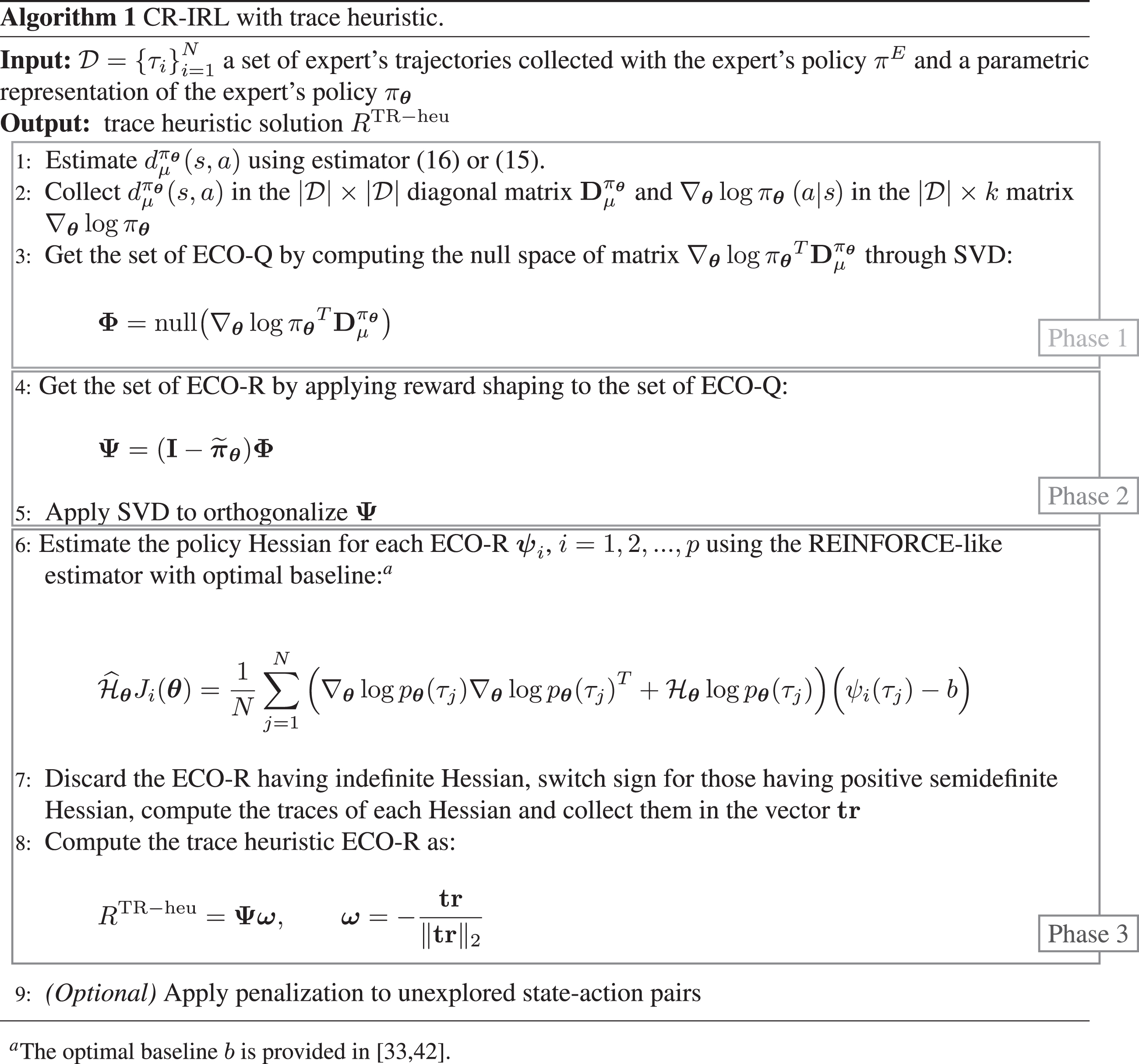
CR-IRL does not assume to know the state space $S$ and the action space $A$ , thus the recovered reward is defined only in the state-action pairs visited by the expert along the trajectories in $D$ . When the state and action spaces are known, we can complete the reward function also for unexplored state-action pairs assigning a penalized reward (e.g., a large negative value), otherwise the penalization can be performed online when the recovered reward is used to solve the forward RL problem.

Refer to Algorithm 1 for a complete overview of CR-IRL.

7 Theoretical analysis

In this section, we provide an analysis of the computational complexity of CR-IRL together with a finite-sample analysis of the feature extraction phase.

7.1 Computational complexity analysis

The main sources of computational complexity in CR-IRL are the SVD, the computation of the Hessian and its eigenvalue computation for each ECO-R. For an m × n matrix it is well known that SVD has complexity $O (\min {{mn}^{2}, {nm}^{2}})$ . We apply SVD twice: the first time it is applied to matrix $\nabla_{θ} log {π_{θ}}^{T} D_{μ}^{π_{θ}}$ of dimension $k \times | D |$ and the second time to matrixΨ of dimension $| D | \times | D |$ at most. Assuming $k \leq | D |$ , the second application dominates yielding a complexity of $O (| D |^{3})$ . The computation of the Hessian is linear in the number of ECO-Rs (at maximum $| D |$ ) and in the number of samples ( $| D |$ ) and quadratic in the number of parameters k, thus the complexity is $O (k^{2} | D |^{2})$ . Finally, the computation of the eigenvalues is cubic in the order of the matrix (k) and has to be done for every ECO-R, yielding a cost of $O (k^{3} | D |)$ , which is dominated by $O (k^{2} | D |^{2})$ as $k \leq | D |$ . Overall the complexity of CR-IRL is $O (\max {k^{2} | D |^{2}, | D |^{3}})$ .

7.2 Finite-sample analysis

In this section, we perform an error analysis of the feature extraction phase. In particular, our goal is to bound the ℓ²-norm of the difference between an ECO-Rψ extracted using the actual expert policy π^E and an infinite number of samples and an approximate ECO-R $\hat{ψ}$ obtained by using our approximation of the expert’s policy π_θ (e.g., the maximum likelihood policy) and a finite number N of samples. We will make use of the following assumptions.

Assumption 7.1. The following statements are assumed to hold:

the state space $S$ and the action space $A$ are finite;

the expert’s policy π^E belongs to Π_Θ, i.e., there exists θ^E ∈ Θ such that π^E = π_{θ
^E};

for any policy π_θ ∈ Π_Θ, for any $s \in S$ , $a \in A$ and for any l = 1, 2, …, k, it holds that | ∇ _{θ
_l} log π_θ (a|s) | ≤ G; 7

the ∇_θ log π_θ is Lipschitz continuous w.r.t. the policy π_θ in the following sense: $| \nabla_{θ} log π_{θ} - \nabla_{θ} log π_{θ^{'}} |_{2} \leq L | π_{θ} - π_{θ^{'}} |_{2} .$

We start by analyzing the error propagation for the ECO-Qs. Our goal is to provide a bound for the ℓ²-norm of the difference between a given ECO-Qϕ and its estimate $\hat{ϕ}$ . We present a general statement about null spaces of matrices.

Lemma 7.1. Let W and $\hat{W}$ be two m × n matrices with m < n. Then, for any vector ϕ ∈ null (W) such that |ϕ|₂ = 1, there exist a vector $\hat{ϕ} \in null (\hat{W})$ , such that: $| ϕ - \hat{ϕ} |_{2} \leq \frac{| W - \hat{W} |_{2}}{σ_{min} (\hat{W})},$ where σ_min (·) denotes the minimum non-zero singular value of a matrix.

Proof. ϕ and $\hat{ϕ}$ are in the null space of matrices W and $\hat{W}$ respectively, thus it holds: $W ϕ = 0, \hat{W} \hat{ϕ} = 0 .$ We can write $\hat{W} = W + ε_{W}$ and $\hat{ϕ} = ϕ + ε_{ϕ}$ , thus: $\begin{matrix} \hat{W} \hat{ϕ} & = (W + ε_{W}) (ϕ + ε_{ϕ}) & = W ϕ + W ε_{ϕ} + ε_{W} ϕ + ε_{W} ε_{ϕ} \\ = W ε_{ϕ} + ε_{W} ϕ + ε_{W} ε_{ϕ} = 0 . \end{matrix}$ (27) Therefore we need to solve the following system of equations for ε _ϕ : $(W + ε_{W}) ε_{ϕ} = - ε_{W} ϕ .$ (28) This is a rectangular system with m equations and n unknowns (the system might be underdeterminated). Among all the solutions we seek for the least-norm solution as we are looking for the smallest perturbation of a given ϕ. The least-norm solution ε _ϕ _LN can be found using the Moore-Penrose pseudoinverse: $ε_{ϕ_{LN}} = - (W + ε_{W})^{†} ε_{W} ϕ .$ (29) Considering that |ϕ|₂ = 1 and passing to the ℓ²-norm we get: $| {ε_{ϕ}}_{LN} |_{2} \leq | (W + ε_{W})^{†} |_{2} | ε_{W} |_{2} .$ (30) Now we need to bound the term $| (W + ε_{W})^{†} |_{2} = | {\hat{W}}^{†} |_{2}$ . It can be proved that, for a generic matrix A [7]: $| A^{†} |_{2} = \frac{1}{σ_{min} (A)},$ (31) where σ_min (A) is the smallest non-zero singular value of matrix A. Therefore, we get the bound: $| {ε_{ϕ}}_{LN} |_{2} \leq \frac{| ε_{W} |_{2}}{σ_{min} (\hat{W})} .$ (32) □

If we take $W = \nabla_{θ} log π_{θ^{E}}^{T} D_{μ}^{π_{θ^{E}}}$ and $\hat{W} = \nabla_{θ} log π_{θ}^{T} {\hat{D}}_{μ}^{π_{θ^{E}}}$ , Lemma 7.1 tells us that, given an ECO-Q ϕ, we can always find an ECO-Q $\hat{ϕ}$ , obtained with finite samples and an approximation of the expert’s policy not too different from ϕ.

As intuition suggests, a more precise estimation of matrix W induces a smaller error in the computation of the ECO-Qs. Therefore, in order to reduce the error we can improve the estimation of W by collecting more expert’s trajectories (if possible) or selecting a better policy space to represent the expert’s behavior. However, the presence of $σ_{min} (\hat{W})$ at the denominator suggests that we can select a policy model (even if more imprecise) in order to increase $σ_{min} (\hat{W})$ . Clearly, a more imprecise model is likely to increase the error $| W - \hat{W} |_{2}$ . Thus, we have to trade-off between the value of $σ_{min} (\hat{W})$ and the error $| W - \hat{W} |_{2}$ . Under the assumption that W and $\hat{W}$ have the same rank, exploiting a standard result from singular values perturbation theory we can provide the following bound on the singular values [7]: $| σ_{min} (\hat{W}) - σ_{min} (W) | \leq | W - \hat{W} |_{2} .$

The ℓ²-norm of the difference between W and $\hat{W}$ can be further bounded as shown in the following result.

Lemma 7.2. Let π_{θ
^E} ∈ Π_Θ be the expert’s policy and π_θ ∈ Π_Θ an arbitrary policy. Let us denote with $W = \nabla_{θ} log π_{θ^{E}}^{T} D_{μ}^{π_{θ^{E}}}$ and $\hat{W} = \nabla_{θ} log π_{θ}^{T} {\hat{D}}_{μ}^{π_{θ^{E}}}$ , where $D_{μ}^{π_{θ^{E}}} = diag (d_{μ}^{π_{θ^{E}}})$ and ${\hat{D}}_{μ}^{π_{θ^{E}}} = diag ({\hat{d}}_{μ}^{π_{θ^{E}}})$ . Then, under Assumption 7.1 it holds that: $\begin{matrix} | W - \hat{W} |_{2} & \leq \sqrt{| S | | A | k} G | {\hat{d}}_{μ}^{π_{θ^{E}}} - d_{μ}^{π_{θ^{E}}} |_{\infty} \\ + L | π_{θ^{E}} - π_{θ} |_{\infty}^{1 / 2} . \end{matrix}$

Proof. $\begin{matrix} W - \hat{W} & = \nabla_{θ} log π_{θ^{E}}^{T} D_{μ}^{π_{θ^{E}}} - \nabla_{θ} log π_{θ}^{T} {\hat{D}}_{μ}^{π_{θ^{E}}} \\ = \nabla_{θ} log π_{θ^{E}}^{T} (D_{μ}^{π_{θ^{E}}} - {\hat{D}}_{μ}^{π_{θ^{E}}}) & + (\nabla_{θ} log π_{θ^{E}}^{T} - \nabla_{θ} log π_{θ}^{T}) {\hat{D}}_{μ}^{π_{θ^{E}}} . \end{matrix}$ Tacking the ℓ²-norm we get: $\begin{matrix} | W - \hat{W} |_{2} & \leq | \nabla_{θ} log π_{θ^{E}} |_{2} | D_{μ}^{π_{θ^{E}}} - {\hat{D}}_{μ}^{π_{θ^{E}}} |_{2} & + | \nabla_{θ} log π_{θ^{E}}^{T} - \nabla_{θ} log π_{θ}^{T} |_{2} | {\hat{D}}_{μ}^{π_{θ^{E}}} |_{2} \\ \leq \sqrt{| S | | A | k} G | {\hat{d}}_{μ}^{π_{θ^{E}}} - d_{μ}^{π_{θ^{E}}} |_{\infty} \\ + L | π_{θ^{E}} - π_{θ} |_{2} \\ \leq \sqrt{| S | | A | k} G | {\hat{d}}_{μ}^{π_{θ^{E}}} - d_{μ}^{π_{θ^{E}}} |_{\infty} \\ + L \sqrt{| π_{θ^{E}} - π_{θ} |_{\infty}}, \end{matrix}$ where we have exploited the property |X^T|₂ = |X|₂ and for an n × m matrix we have $| X |_{2} = \sqrt{nm} | X |_{max}$ . Furthermore, we used the fact that $D_{μ}^{π_{θ}} = diag (d_{μ}^{π_{θ}})$ and therefore $| D_{μ}^{π_{θ^{E}}} |_{2} = | d_{μ}^{π_{θ^{E}}} |_{\infty} \leq 1$ and similarly for $| D_{μ}^{π_{θ^{E}}} - {\hat{D}}_{μ}^{π_{θ^{E}}} |_{2} = | d_{μ}^{π_{θ^{E}}} - {\hat{d}}_{μ}^{π_{θ^{E}}} |_{\infty}$ . Finally, we exploited the fact that $| X |_{2} \leq \sqrt{| X |_{1} | X |_{\infty}}$ and used the fact that |π_{θ
^E} - π_θ|₁ ≤ 1.□

We can now provide a finite-sample bound for the quantity $| {\hat{d}}_{μ}^{π_{θ^{E}}} - d_{μ}^{π_{θ^{E}}} |_{1}$ , recalling that for a vector v we have |v|_∞ ≤ |v|₁.

Lemma 7.3. For any δ ∈ (0, 1], with probability at least 1 - δ, for estimator (16) it holds that: $\begin{matrix} | {\hat{d}}_{μ}^{π_{θ^{E}}} - d_{μ}^{π_{θ^{E}}} |_{1} \leq 2 γ^{H} + | π_{θ^{E}} - π_{θ} |_{\infty} \\ + \sqrt{\frac{2 [log (2^{| S |} - 2) + log \frac{1}{δ}]}{N}}, \end{matrix}$ and for estimator (15) it holds that: $\begin{matrix} | {\hat{d}}_{μ}^{π_{θ^{E}}} - d_{μ}^{π_{θ^{E}}} |_{1} \leq 2 γ^{H} \\ + \sqrt{\frac{2 [log (2^{| S | | A |} - 2) + log \frac{1}{δ}]}{N}} . \end{matrix}$

Proof. Let us start with the estimator (16), we have: $\begin{matrix} {π_{θ}}^{T} {\hat{d}}_{μ}^{π_{θ^{E}}} & - π_{θ^{E}}^{T} d_{μ}^{π_{θ^{E}}} = {(π_{θ} - π_{θ^{E}})}^{T} {\hat{d}}_{μ}^{π_{θ^{E}}} \\ + π_{θ^{E}}^{T} ({\hat{d}}_{μ}^{π_{θ^{E}}} - d_{μ}^{π_{θ^{E}}}) . \end{matrix}$ Passing to the ℓ¹-norm, and recalling that |X^T|₁ = |X|_∞ we get: $\begin{matrix} | {π_{θ}}^{T} {\hat{d}}_{μ}^{π_{θ^{E}}} & - π_{θ^{E}}^{T} d_{μ}^{π_{θ^{E}}} |_{1} \leq | π_{θ} - π_{θ^{E}} |_{\infty} | {\hat{d}}_{μ}^{π_{θ^{E}}} |_{1} \\ + | π_{θ^{E}} |_{\infty} | {\hat{d}}_{μ}^{π_{θ^{E}}} - d_{μ}^{π_{θ^{E}}} |_{1} \\ \leq | π_{θ} - π_{θ^{E}} |_{\infty} + | {\hat{d}}_{μ}^{π_{θ^{E}}} - d_{μ}^{π_{θ^{E}}} |_{1} . \end{matrix}$ Notice that the estimator ${\hat{d}}_{μ}^{π_{θ^{E}}}$ is biased as it is cut at horizon H< + ∞. We indicate with $d_{μ, H}^{π_{θ^{E}}}$ the vector of the γ-discounted state distribution cut at horizon H defined as: $d_{μ, H}^{π_{θ^{E}}} (s) = \frac{1 - γ}{1 - γ^{H}} \sum_{t = 0}^{H - 1} γ^{t} Pr (s_{t} = s | π_{θ}) .$ (33) Thus, ${\hat{d}}_{μ}^{π_{θ^{E}}}$ is an unbiased estimator for $d_{μ, H}^{π_{θ^{E}}}$ . By applying [58] we have the following finite-sample bound, that holds with at least probability 1 - δ, δ ∈ (0, 1]: $| {\hat{d}}_{μ}^{π_{θ^{E}}} - d_{μ, H}^{π_{θ^{E}}} |_{1} \leq \sqrt{\frac{2 (log (2^{| S |} - 2) + log \frac{1}{δ})}{N}} .$ Now we need to account for the bias, bounding the term $| d_{μ}^{π_{θ^{E}}} - d_{μ, H}^{π_{θ^{E}}} |_{1}$ : $\begin{matrix} | & d_{μ}^{π_{θ^{E}}} - d_{μ, H}^{π_{θ^{E}}} |_{1} = \sum_{s \in S} | (1 - γ) \sum_{t = 0}^{+ \infty} γ^{t} Pr (s_{t} = s | π_{θ}) \\ - \frac{1 - γ}{1 - γ^{H}} \sum_{t = 0}^{H - 1} γ^{t} Pr (s_{t} = s | π_{θ}) | \\ \leq (1 - γ) \sum_{s \in S} | \sum_{t = H}^{+ \infty} γ^{t} Pr (s_{t} = s | π_{θ}) | \\ + \frac{1 - γ}{1 - γ^{H}} γ^{H} \sum_{s \in S} | \sum_{t = 0}^{H - 1} γ^{t} Pr (s_{t} = s | π_{θ}) | \\ \leq (1 - γ) \sum_{t = H}^{+ \infty} γ^{t} \sum_{s \in S} Pr (s_{t} = s | π_{θ}) \\ + \frac{1 - γ}{1 - γ^{H}} γ^{H} \sum_{t = 0}^{H - 1} γ^{t} \sum_{s \in S} Pr (s_{t} = s | π_{θ}) \\ = (1 - γ) \sum_{t = H}^{+ \infty} γ^{t} + \frac{1 - γ}{1 - γ^{H}} γ^{H} \sum_{t = 0}^{H - 1} γ^{t} \\ = (1 - γ) \frac{γ^{H}}{1 - γ} + \frac{1 - γ}{1 - γ^{H}} γ^{H} \frac{1 - γ^{H}}{1 - γ} = 2 γ^{H}, \end{matrix}$ where we exploited the fact that $\sum_{s \in S} Pr (s_{t} = s | π_{θ}) = 1$ for every t and we used the properties of the geometric series. Observing that $| {\hat{d}}_{μ}^{π_{θ^{E}}} - d_{μ}^{π_{θ^{E}}} |_{1} \leq | {\hat{d}}_{μ}^{π_{θ^{E}}} - d_{μ, H}^{π_{θ^{E}}} |_{1} + | d_{μ, H}^{π_{θ^{E}}} - d_{μ}^{π_{θ^{E}}} |_{1}$ and putting all together we get the result.

For the estimator (15), the derivation is analogous. We do not have to decompose the contribution of the policy, but we just need to bound the bias (the proof is identical to the one presented above, just summing over the state-action space) and apply [58] recalling that this second estimator is defined over the state-action space.□

The following result provides a bound of the ℓ²-norm of the error in the estimation of an ECO-R ψ given the ℓ²-norm of error in the estimation of the corresponding ECO-Q ϕ.

Theorem 7.1. Let π_{θ
^E} ∈ Π_Θ be the expert’s policy and π_θ ∈ Π_Θ an arbitrary policy. Let us denote with $W = \nabla_{θ} log π_{θ^{E}}^{T} D_{μ}^{π_{θ^{E}}}$ and $\hat{W} = \nabla_{θ} log π_{θ}^{T} {\hat{D}}_{μ}^{π_{θ^{E}}}$ , where $D_{μ}^{π_{θ^{E}}} = diag (d_{μ}^{π_{θ^{E}}})$ and ${\hat{D}}_{μ}^{π_{θ^{E}}} = diag ({\hat{d}}_{μ}^{π_{θ^{E}}})$ . Then, under Assumption 7.1 it holds that: $\begin{matrix} | ψ - \hat{ψ} |_{2} & \leq (1 + \sqrt{| A |}) | ϕ - \hat{ϕ} |_{2} \\ + \sqrt{| A |} | π_{θ^{E}} - π_{θ} |_{\infty}^{1 / 2} . \end{matrix}$

Proof. $\begin{matrix} ψ - \hat{ψ} & = (I - {\tilde{π}}_{θ^{E}}) ϕ - (I - {\tilde{π}}_{θ}) \hat{ϕ} \\ = (ϕ - \hat{ϕ}) - {\tilde{π}}_{θ} (ϕ - \hat{ϕ}) + ({\tilde{π}}_{θ} - {\tilde{π}}_{θ^{E}}) ϕ . \end{matrix}$ (34) Tacking the ℓ²-norm we get: $\begin{matrix} | ψ - \hat{ψ} |_{2} & \leq | ϕ - \hat{ϕ} |_{2} + | {\tilde{π}}_{θ} |_{2} | ϕ - \hat{ϕ} |_{2} \\ + | {\tilde{π}}_{θ} - {\tilde{π}}_{θ^{E}} |_{2} | ϕ |_{2} \\ \leq | ϕ - \hat{ϕ} |_{2} + \sqrt{| A |} | ϕ - \hat{ϕ} |_{2} \\ + \sqrt{| A | | {\tilde{π}}_{θ} - {\tilde{π}}_{θ^{E}} |_{\infty}} \\ \leq | ϕ - \hat{ϕ} |_{2} + \sqrt{| A |} | ϕ - \hat{ϕ} |_{2} \\ + \sqrt{| A | | π_{θ} - π_{θ^{E}} |_{\infty}}, \end{matrix}$ where we have exploited the fact that $| X |_{2} \leq \sqrt{| X |_{1} | X |_{\infty}}$ and $| {\tilde{π}}_{θ} |_{\infty} = 1$ being a stochastic matrix and $| {\tilde{π}}_{θ} |_{1} \leq | A |$ by definition of $\tilde{π}$ and that $| {\tilde{π}}_{θ} - {\tilde{π}}_{θ^{E}} |_{\infty} = | π_{θ} - π_{θ^{E}} |_{\infty}$ .□

As the ECO-Rs are computed starting from the ECO-Qs by means of a linear mapping involving the policy, the bound depends not only on the error in the estimation of the ECO-Qs but also on the error in the policy representation. It is worth to notice that this transformation is likely to amplify the error due to the multiplication for $1 + \sqrt{| A |}$ which is clearly not smaller than 2.

8 Related works

IRL approaches can be classified according to several dimensions. A first notable dichotomy is between model-based and model-free algorithms. The former, such as [39, 52, 62], are hardly deployable to real-world applications since they require to have access to a representation of the environment transition model P. The estimation of the transition model is particularly challenging when the state (or action) space is continuous, but it is even more difficult if we have only expert’s demonstrations at our disposal. An expert is typically an optimal (or near-optimal) agent, thus it is going to explore a very limited region of the state space, resulting in poor estimation of the transition model. As an alternative, we could collect trajectories using an explorative (e.g., random) policy, but this would potentially increase the execution cost. Other methods, like feature expectation algorithms [1, 53], do not require explicitly the transition model even if they need to sample the environment in order to solve the forward reinforcement learning problem. These algorithms belong to a gray zone in between model-based and model-free.

A limited number of algorithms can be defined really model-free. On one hand, structured classification methods [27, 28] deal with the IRL problem with no need for interaction with the environment, apart from collecting expert’s demonstrations. These methods cast the problem of recovering the reward function into a multi-class classification problem, possibly formulated in multiple stages [28]. The approaches based on the policy gradient, like GIRL [45], SOME-IRL [54] and CR-IRL [36] are able to recover a reward function from a set of expert’s trajectories only, as well. However, these methods, differently to the structured classification approaches that resort to supervised learning, explicitly take advantage of the structure of the underlying MDP.

Another relevant issue is reward ambiguity. The choice of a reward function among all feasible ones is, of course, related to the notion of optimality we decide to employ. Indeed, literature has not treated this issue in a comprehensive way yet. Intuitively, we aim to find a reward with “good” learning properties, i.e., a reward able to learn the optimal policy quickly. However, the learning speed is an algorithm-dependent property. Maximum Entropy Inverse Reinforcement Learning (ME-IRL) [61, 62] dealt with this issue explicitly, proposing an optimality criterion based on the maximum entropy principle, in which we prefer a reward function that imposes as few constraints as possible on the optimal policy if not justified by the expert’s choices. Similarly, Relative Entropy Inverse Reinforcement Learning (RE-IRL) [10] extends ME-IRL removing the need of knowing the full environment model, still requiring a dataset collected with an explorative policy.

The choice of the reward approximation space is a further issue. Early IRL methods had a preference for linear parametrizations, most of them work with linear parametrizations only [e.g., 1, 52]. Resorting to linear models is risky for, essentially, two reasons. First, a linear model might not be able to learn the possibly complex dynamics going on in the features. Second, a bad choice of the features might harm the process of reward recovery. Research tried to tackle both problems. Algorithms able to generate automatically the feature space overcome the latter problem. Indeed, with a good feature construction mechanism, even a linear model is effective. Instead, linear approximators are replaced with expressive non-linear neural networks in deep learning approaches to IRL [e.g., 16, 21, 23] which are able to deal with both problems at once. These approaches, however, tend not to fully exploit the Markovian nature of the underlying environment. In particular, in [16], Guided Cost Learning is proposed to deal with the IRL problem in complex continuous environment without assuming the knowledge of the true environment model, by employing deep function approximates. The algorithm extends ME-IRL and combines forward RL. The idea behind this approach is to progressively change the sampling distribution in order to match the maximum entropy distribution. In this way, the algorithm exploits the expressive power of the neural networks to learn, jointly, the features and the reward function. Differently, CR-IRL keeps the feature construction and the reward selection phases separated and performs them in sequence. For this reason, once we extracted the informative features for the reward (ECO-R) we can simply use linear models for building the reward function, without making use of complex function approximators. In the same direction of extending ME-IRL, in [17] Adversarial Inverse Reinforcement Learning (AIRL) is presented as an approach based on the adversarial framework [20] that allows learning the reward function and the value function simultaneously. The authors claim that by using a reward function depending on the state only, they are able to mitigate the ambiguity problem by learning rewards that are independent from the underlying environment dynamics. Similarly, in [56] an approach to tackle the IRL problem in Linearly solvable MDPs [55] is presented. The IRL problem is formulated as a density ratio estimation between the optimal state transition and a baseline and, finally, solved via logistic regression.

At best of our knowledge, the only IRL method that directly tackles the feature construction problem is Feature Construction for Inverse Reinforcement Learning (FIRL) [29]. FIRL alternates between optimization and fitting phases. The optimization phase aims to recover a reward function, from the current feature set as a linear projection, such that the associated optimal policy is consistent with the demonstrations. In the fitting phase, new features are created (using a regression tree) in order to better explain regions where the old features were too coarse. The method proved to be effective in achieving also (features) transfer capabilities. However, FIRL requires the MDP model to solve the forward problem and the complete optimal policy for the fitting step in order to evaluate the consistency with demonstrations. We believe that this might represent a significant limitation, especially in scenarios in which accessing the environment is costly, dangerous or even impossible (e.g., critical industrial applications). Differently, CR-IRL is fully model-free, being able to recover an approximation space for the reward function and selecting a unique reward within this space, by employing the set of expert’s demonstrations solely.

9 Experimental evaluation

This section is devoted to the experimental evaluation of CR-IRL on classic benchmark problems, both discrete and continuous: the Taxi problem (Section 9.2), the Linear Quadratic Gaussian Regulator (Section 9.3) and the Car on the Hill environment (Section 9.4).

We compare CR-IRL with classic IRL algorithms in order to evaluate the performance of the recovered reward functions. In particular, the experiments are intended to evaluate both the phases of CR-IRL: the feature construction and the reward recovery. For the feature construction phase, we compare the ECO-R with a predetermined set of features automatically generated (like Proto-Value Function, PVFs [31]); while for the reward recovery phase we evaluate CR-IRL against popular state-of-the-art IRL algorithms able to output a reward as a linear combination of features when fed with ECO-R.

We start presenting the evaluation metrics we adopt to compare the considered algorithms (Section 9.1) and then we report the full results of the experiments.

9.1 Evaluation metrics

Defining a metric to evaluate the intuitive notion of “good reward” is a hard task and literature has not formalized it yet. Intuition suggests that we should recover a reward function that allows the agent to learn a policy as close as possible to the expert’s policy. However, there are problems in which even if the learned policy and the expert’s policy are significantly different the average return is very close, and vice versa. In other words, a small policy deviation might attain a large return deviation. Furthermore, all other things being equal, we should prefer a reward function with a faster learning curve. Clearly, this last property is algorithm-dependent. For these reasons we resort to multiple metrics:

learning speed: the number of iterations of the forward RL algorithm needed for converging to the optimal policy;

average return: the average return $\hat{J}$ of the policy learned with the recovered reward function, compared with the expert’s average return J^E;

policy distance: the distance between the expert’s policy π^E and the learned policy $\hat{π}$ (Kullback-Leibler divergence);

parameter distance: when both the expert’s policy and the learned policy are parametric policies of the same class, the distance (in norm) between the expert’s parameters θ^E and the learned parameters $\hat{θ}$ . 8

9.2 Taxi

This section is devoted to the experiments performed on the Taxi domain, defined in [13]. The environment corresponds to a 5×5 grid in which there are 4 locations, labeled by different letters (R, G, B, and Y). The job of the taxi driver is to pick up the passenger at one location and drop him off in another. The agent receives +20 points for a successful dropoff and loses 1 point for every timestep it takes. There is also a 10 point penalty for illegal pick-up and drop-off actions. The available actions are the movements in the four directions (North, East, South, West), pick-up and drop-off (all actions are deterministic). The passenger position, the destination position and the initial position of the taxi represent the state. The distribution of the initial state is uniform and the discount factor is 0.99.

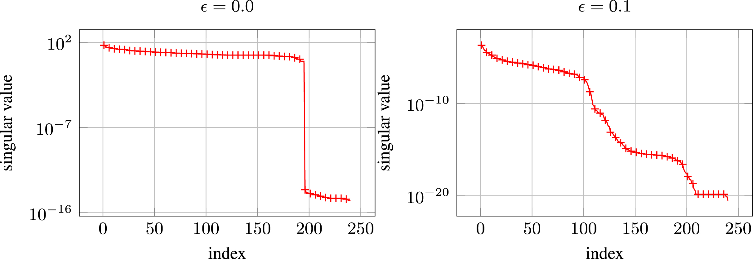
We compute the optimal deterministic policy via value iteration [6] and we use it to fit, via maximum likelihood (with ridge regularization on the parameters), the parameters of expert’s policy, belonging to the class of ε-Boltzmann policies with fixed ε: 9 $π_{θ, ε} (a | s) = (1 - ε) \frac{e^{θ_{a}^{T} ζ_{s}}}{\sum_{a^{'} \in A} e^{θ_{a^{'}}^{T} ζ_{s}}} + \frac{ε}{| A |},$ (35) where the policy features ζ_s are the following state features: current location, passenger location, destination location, whether the passenger has already been picked up. In order to test the robustness of CR-IRL to imperfect experts we introduce a noise ε in the expert’s policy (also named exploration level in the following). We consider the cases ε = 0 and ε = 0.1. The resulting policy has 240 parameters, however the policy rank is smaller (195 for ε = 0 and 185 for ε = 0.1) due to the presence of parameters that do not affect the policy performance (Fig. 1).

Fig. 1

Singular values of the ∇_θ log π_θ,ε. When ε = 0 the gap between non-zero and zero singular values is clear; while the behavior is smoother when ε = 0.1 but the magnitude of the singular values is significantly smaller.

We compare the performance of CR-IRL with trace heuristics criterion, 10 against Behavioral Cloning (BC), obtained by recovering the maximum likelihood Boltzmann policy from expert’s trajectories, Maximum Entropy IRL (ME-IRL) [62], Relative Entropy IRL (RE-IRL) [10] and Linear Programming Apprenticeship Learning (LPAL) [52].

In order to recover the set of ECO-R we collect 100 expert’s trajectories. For this experiment we evaluate both model-free and model-based versions of CR-IRL. For the latter case the transition model is estimated from expert’s trajectories via the Monte Carlo estimator:

$\begin{matrix} \hat{P} (s^{'} | s, a) = \\ \frac{\sum_{i = 1}^{N} \sum_{t = 0}^{H - 1} 1 ((s_{τ_{i}, t + 1}, a_{τ_{i}, t}, s_{τ_{i}, t}) = (s^{'}, a, s))}{\sum_{i = 1}^{N} \sum_{t = 0}^{H - 1} 1 ((a_{τ_{i}, t}, s_{τ_{i}, t}) = (a, s))} . \end{matrix}$ (36)

Implementation issues. In the Taxi domain when the agent reaches the terminal state it will receive zero reward forever. However, the reward function recovered by CR-IRL could assign a non-zero reward to the terminal state. For implementation reasons, we translate the recovered reward in order to ensure zero-reward to the terminal state. Furthermore, the recovered reward function is extended to the unvisited state-action pairs assigning the minimum value among the rewards of the visited state-action pairs.

Learning speed experiments. This set of experiments is meant to compare the learning speed of the reward functions recovered by the considered IRL methods when a Boltzmann policy (ε = 0) is trained with REINFORCE [59]. The training is performed with Adam [26] (learning rate 0.008, other parameters with default value), at each iteration 100 trajectories are used to estimate the gradient and the initial parameter is θ⁽⁰⁾ = 0 so that the initial policy $π_{θ, 0}^{(0)}$ is the random uniform policy. 11 All data are averaged over 40 runs and the error bars correspond to the 95% confidence intervals.

Figure 2 shows that model-free CR-IRL, with 100 expert’s trajectories, outperforms the original reward function in terms of convergence speed regardless of the exploration level. Behavioral Cloning (BC), obtained by recovering the maximum likelihood ε-Boltzmann policy from expert’s trajectories, is very susceptible to noise, as expected, for both values of ε. Similarly, Linear Programming Apprenticeship Learning (LPAL) [52] using as reward features the set of model-free ECO-R is unable to reach the optimal performance. Indeed, LPAL provides as output an apprenticeship policy (not a reward function) and, like BC, is very sensitive to noise and to the quality of the estimated transition model.

Fig. 2

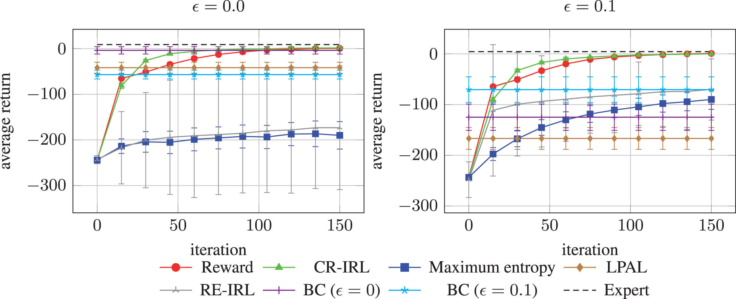
Average return of the Taxi problem as a function of the number of iterations of REINFORCE for model-free ECO-R.

We also compare, in Fig. 2, the second-order criterion of CR-IRL to single out the reward function with Maximum Entropy IRL (ME-IRL) [62] and Relative Entropy IRL (RE-IRL) [10] using as reward features the set of model-free ECO-R. We can see in Fig. 2 that ME-IRL does not perform well when ε = 0, since the transition model is badly estimated. A similar behavior, with even larger variance, is shown by RE-IRL. The convergence speed remains very slow also for ε = 0.1, since ME-IRL does not guarantee that the recovered reward is a maximum of J. Instead, RE-IRL is able to produce a reward that reaches higher performance.

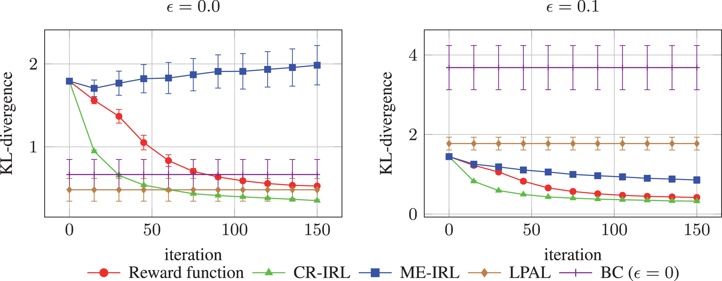
Besides the average return, we compare the recovered reward functions in terms of distance between the expert’s policy π^E and the learned policy π_θ (Kullback-Leibler divergence) estimated with: ${\hat{D}}_{KL} (π^{E} | π_{θ}) = \frac{1}{N} \sum_{i = 1}^{N} \sum_{t = 0}^{H - 1} log \frac{π^{E} (a_{τ_{i}, t} | s_{τ_{i}, t})}{π_{θ} (a_{τ_{i}, t} | s_{τ_{i}, t})} .$ Figure 3 confirms the faster convergence of CR-IRL over the original reward and ME-IRL. We observe that LPAL is able to recover a policy that is more similar to the expert’s policy w.r.t. that of BC, however the average return is worse (this is a consequence of the fact that LPAL does not learn well to perform pick-up and drop-off actions that are associated with the largest rewards).

Fig. 3

Kullback-Leibler divergence between expert’s policy and learned policy in the Taxi problem as a function of the number of iterations of REINFORCE for model-free ECO-R.

We also test the model-based version of CR-IRL, where the transition model is estimated with (36). In Figs. 4 and 5 we notice that the usage of model-based ECO-R instead of model-free ECO-R has no relevant impact on CR-IRL and LPAL, while ME-IRL benefits from the model-based features only when the expert is not noisy.

Fig. 4

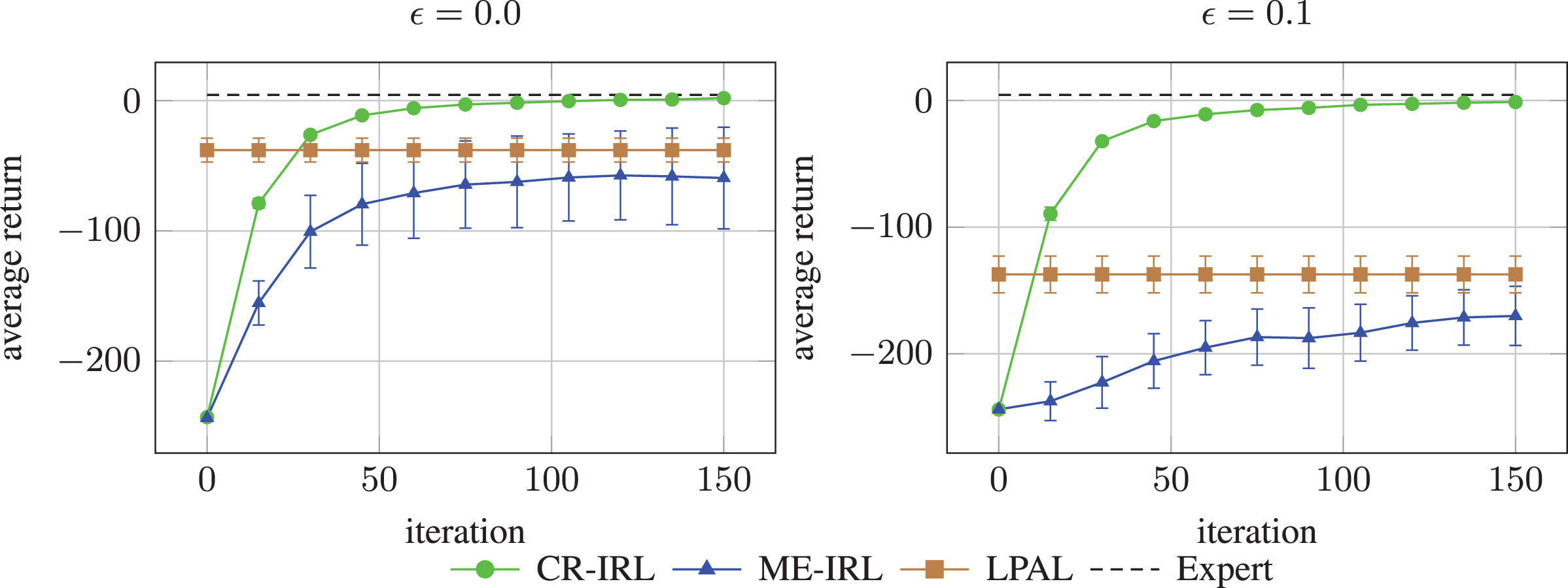
Average return of the Taxi problem as a function of the number of iterations of REINFORCE for reward functions recovered from model-based ECO-Rs.

Fig. 5

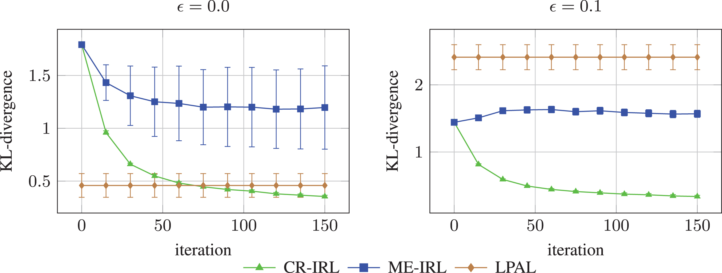
Kullback-Leibler divergence between expert’s policy and learned policy in the Taxi problem as a function of the number of iterations of REINFORCE for model-based ECO-R.

The previous experiments demonstrate that the set of ECO-R constructed by CR-IRL when coped with the trace heuristic criterion allows recovering policies that outperform popular IRL methods and display a faster learning curve w.r.t. the original reward function. The fact that ECO-Rs do not perform well with traditional IRL methods is simply explained. ECO-Rs are built exploiting a first-order optimality condition on the policy gradient with no need of a preselection of an approximation space; traditional IRL methods are designed to deal with handcrafted features that, in some intuitive sense, represent the underlying dynamics of the problem.

The trace heuristic can be also used when a given set of features (different from ECO-R) is provided. Since the usage of the Hessian makes sense only when all the considered features are a stationary point of the policy gradient we first need to remove the orthogonal projections over the space spanned by the gradient log-policy. We compare (Fig. 6) the learning performance of the set of the first 100 Proto-Value Functions (PVF) [30] when linearly combined with ME-IRL, LPAL and our trace heuristic. We notice that LPAL outperforms both the maximum entropy and the Hessian approaches regardless of the exploration level. Trace heuristic is slightly more effective w.r.t. maximum entropy when the expert is not noisy. The poor performance of trace heuristic with predefined approximation space is due to the fact that such space might not be sufficiently expressive to represent a sharp maximum of J.

Fig. 6

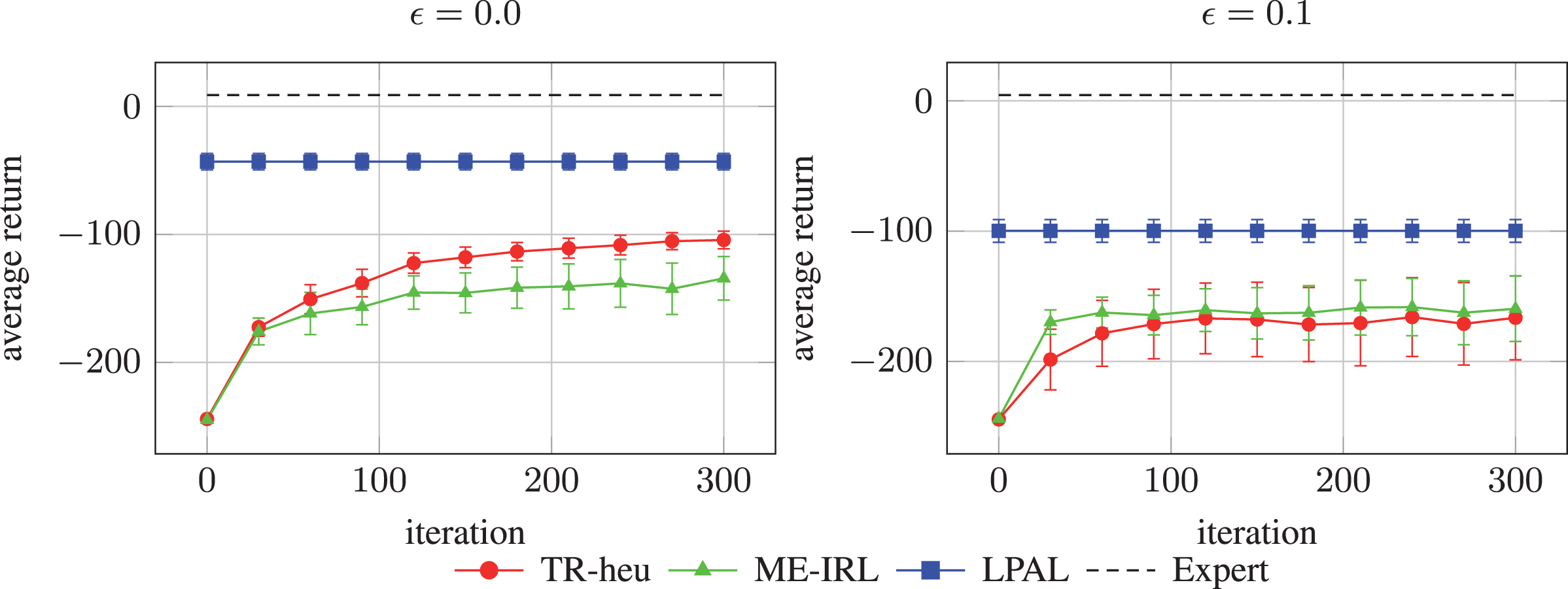
Average return of the Taxi problem as a function of the number of iterations of REINFORCE with the reward function obtained from PVFs.

Overall, we notice that the two phases of CR-IRL (feature construction and reward recovery) are not fully independent because both share a strong relationship to the optimality conditions on the policy gradient and Hessian. In all scenarios, we considered the best performance is obtained with the combination of the two phases.

Sensitivity to the number of expert’s trajectories. The last set of experiments aims at evaluating the effect of the number of expert’s trajectories on the average return of the recovered reward functions (Figs. 7 and 8). The experiment is performed with model-free ECO-R. We notice that CR-IRL is susceptible to the number of expert’s trajectories only when ε = 0.1: the expert demonstrates a suboptimal behavior and this is more likely when the trajectories are many. This reflects on the estimation of the reward function that does not penalize suboptimal actions performed by the expert. LPAL shows the expected behavior, improving the average return as the number of trajectories increases. Also BC improves overall with the number of trajectories, more effectively when the expert is not noisy.

Fig. 7

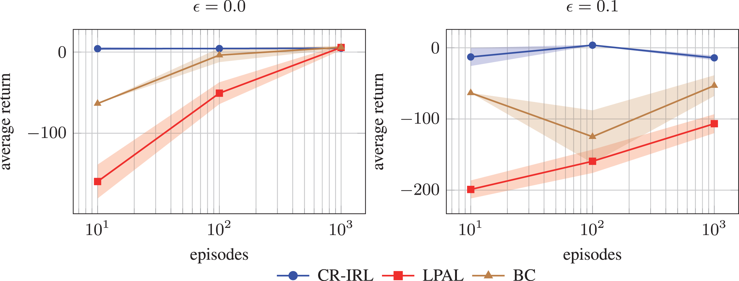
Average return of the Taxi problem as a function of the number of expert’s trajectories.

Fig. 8

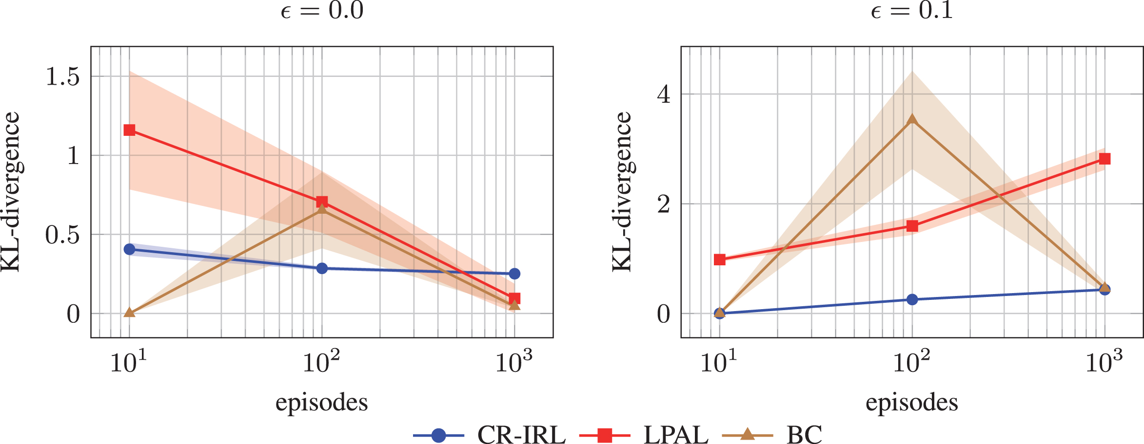
KL-divergence between expert’s policy and learned policy for the Taxi problem as a function of the number of expert’s trajectories.

9.3. Linear quadratic gaussian regulator

The Linear Quadratic Gaussian Regulator (LQG) [14] is a discrete time control problem in a continuous state-action space. The state and reward equations are given by: $\begin{matrix} s_{t + 1} = A s_{t} + B a_{t} + η_{t}, \\ r_{t} = - s_{t}^{T} Q s_{t} - a_{t}^{T} R a_{t}, \end{matrix}$ where A, B, Q and R are coefficient matrices and η_t is a noise process assumed to be a Gaussian white noise $η_{t} \sim N (0, Λ)$ with uncorrelated components Λ = λ² I. The goal of the agent is to reach as soon as possible the origin since it receives, at each time step, a penalization proportional to the magnitude of the state and the action. The optimal control policy in steady state conditions is the linear controller a_t = Ks_t where matrix K can be found by solving the Riccati equation [14]. For the expert’s policy, we consider the class of Gaussian policies $a_{t} \sim N (K s_{t}, Σ)$ with parameter K (Σ is fixed): $a_{t} = K s_{t} + ξ_{t},$ (37) where ξ_t is a Gaussian white noise $ξ_{t} \sim N (0, Σ)$ with uncorrelated components (Σ = σ² I) and uncorrelated with η_t. For implementation reasons, we consider a bounded state-action space $S = [- 10, - 10]^{n}$ , $A = [- 8, 8]^{n}$ , where n is the dimension of the state (and action) space. All components of the initial state are fixed to -4, the discount factor is 0.99 and the trajectory horizon 100. Like in the Taxi problem we consider the case of imperfect expert; we use σ² (policy variance) to tune the degree of exploration of the expert (we consider σ² ∈ {1, 0.01}).

We perform experiments in the one-dimensional case (n = 1, 1D-LQG), the values of the coefficients are reported in Table 1.

Table 1

Coefficients of the 1D-LQG experiments

a	b	q	r	λ ²	k ^*
1.0	1.0	0.9	0.9	0.1	-0.61525

We compare CR-IRL with GIRL using two linear parametrizations of the reward function: \begin flalign*R(s,a,\omega ) = \omega_1 s^2 + \omega_2 a^2 (GIRL-square),\\ R(s,a,\omega ) = \omega_1|s| + \omega_2|a| (GIRL-abs-val). \end flalign*

Tables 2 and 3 show the values of the policy gradient and the policy Hessian computed for the different recovered reward functions. GIRL, by construction, yields the reward functions with the smallest gradient in absolute value. On the contrary, CR-IRL provides a reward function with larger gradient variance; this is justified by the fact that the Hessian is a large negative number making the policy parameter value a very unstable point for the expected return and so the gradient estimation noisier.

Table 2

Policy gradient ∇_θJ (θ) of the recovered reward functions of 1D-LQG for different valuesof σ² (± standard deviation)

Reward function	σ² = 1	σ² = 0.01
Original reward	-0.09203 ± 0.5076	0.03185 ± 0.08893
Advantage function	-0.09356 ± 0.4983	0.9083 ± 1.467
CR-IRL	2.822 ± 10.77	-0.7514 ± 55.45
GIRL-abs-val	(-2.587 ± 1.422) e - 15	(1.858 ± 6.068) e - 14
GIRL-square	(-1.256 ± 1.534) e - 14	(-2.144 ± 5.232) e - 14

Table 3

Policy Hessian $H_{θ} J (θ)$ of the recovered reward functions of 1D-LQG for different values σ² (± standard deviation)

Reward function	σ² = 1	σ² = 0.01
Original reward	-3.064 ± 7.262	-6.371 ± 5.847
Advantage function	-3.601 ± 6.521	-223.1 ± 114.4
CR-IRL	-1854 ± 147.5	-28702 ± 2586
GIRL-abs-val	3.572 ± 12.33	-17.25 ± 32.84
GIRL-square	-0.3941 ± 8.218	-6.213 ± 4.956

In Fig. 9 the recovered reward functions are represented. We can see that GIRL-square is able to recover almost exactly the original reward (but it is very sensitive to the available expert’s trajectories), indeed the original reward function falls into the considered class of rewards. CR-IRL recovers rewards that penalize significantly the disadvantageous regions, this favors the learning speed as the experiments demonstrate. Clearly, as σ² increases the penalized region reduces.

Fig. 9

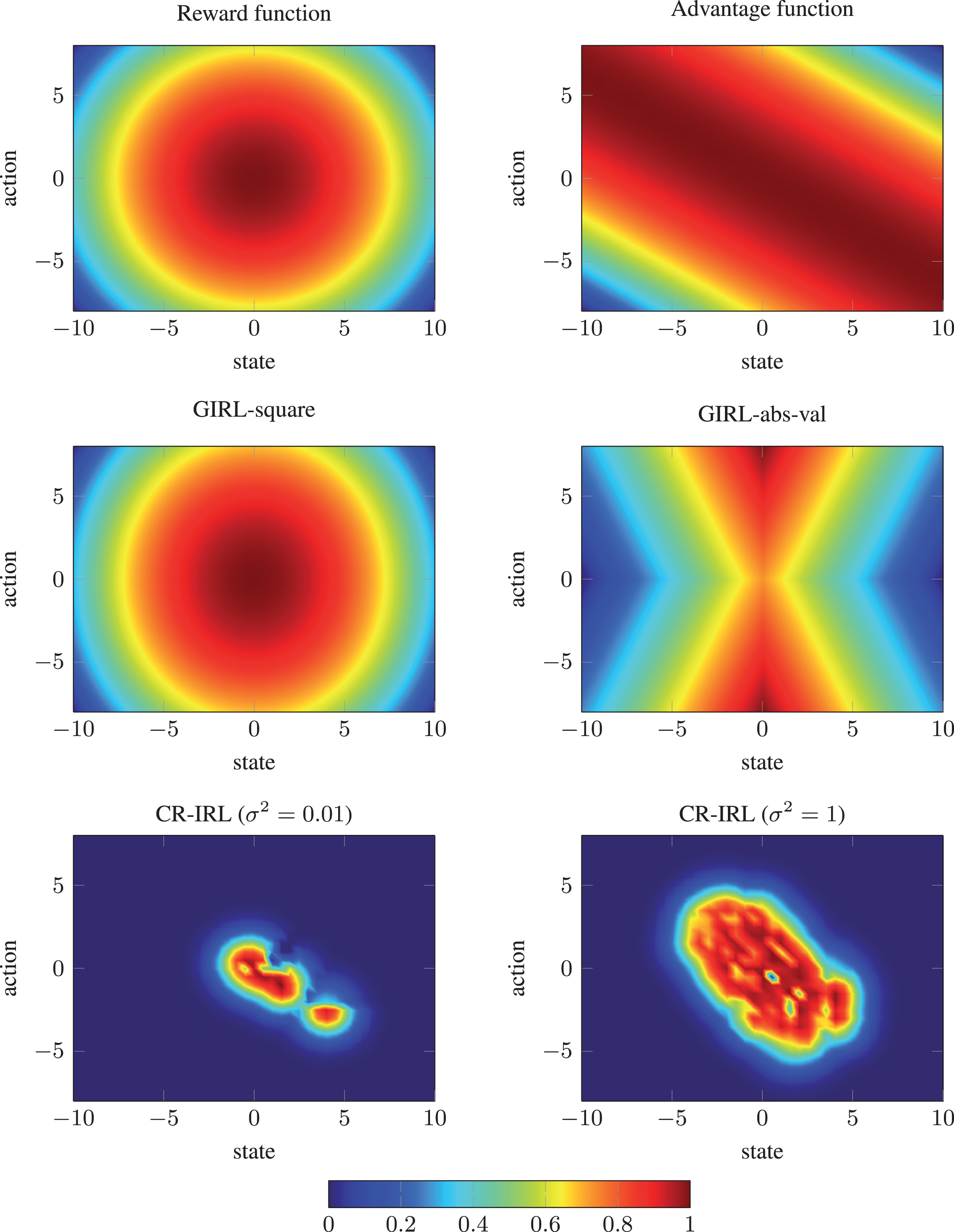
Representation of the recovered reward functions for 1D-LQG.

Learning speed experiments. The training is performed using REINFORCE [59] with Adam [26] (learning rate 0.002, other parameters with default value), at each iteration 100 trajectories are used to estimate the gradient and the initial parameter is k = -0.2. All data are averaged over 40 runs and the error bars correspond to the 95% confidence intervals.

Figure 10 shows the parameter value learned with REINFORCE using a Gaussian policy with two different variances. We notice that CR-IRL, fed with 20 expert’s trajectories, converges closer and faster to the expert’s parameter w.r.t. to the original reward, advantage function and GIRL with both parametrizations when σ² = 0.01. Instead, the convergence value of CR-IRL when the expert is explorative σ² = 1.0 deviates significantly from the optimal value. This however, does not affect the average return, as shown in Fig. 11. Indeed, when the variance is large the effect of the parameter k (the mean of the distribution) on the average return is less relevant.

Fig. 10

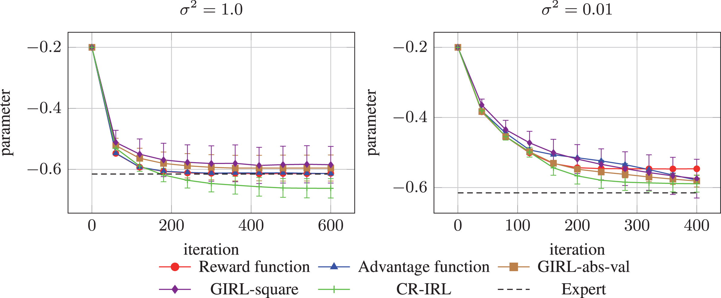
Parameter value of 1D-LQG as a function of the number of iterations of REINFORCE.

Fig. 11

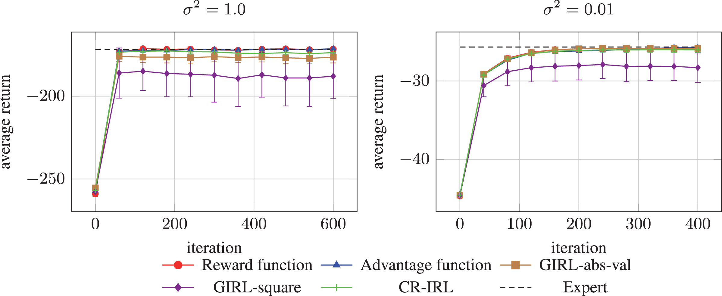
Average return of 1D-LQG as a function of the number of iterations of REINFORCE.

Sensitivity to the number of expert’s trajectories. We investigate the effect of the number of expert’s demonstrations on the performance of the considered IRL algorithms. Fig. 12 reports the convergence parameter value and the average return for a variable number of expert’s trajectories. We notice that CR-IRL is less sensitive w.r.t. to GIRL since, even if few expert’s trajectories are provided, CR-IRL penalizes the regions that the expert did not visit, avoiding the agent to fall into low-reward regions.

Fig. 12

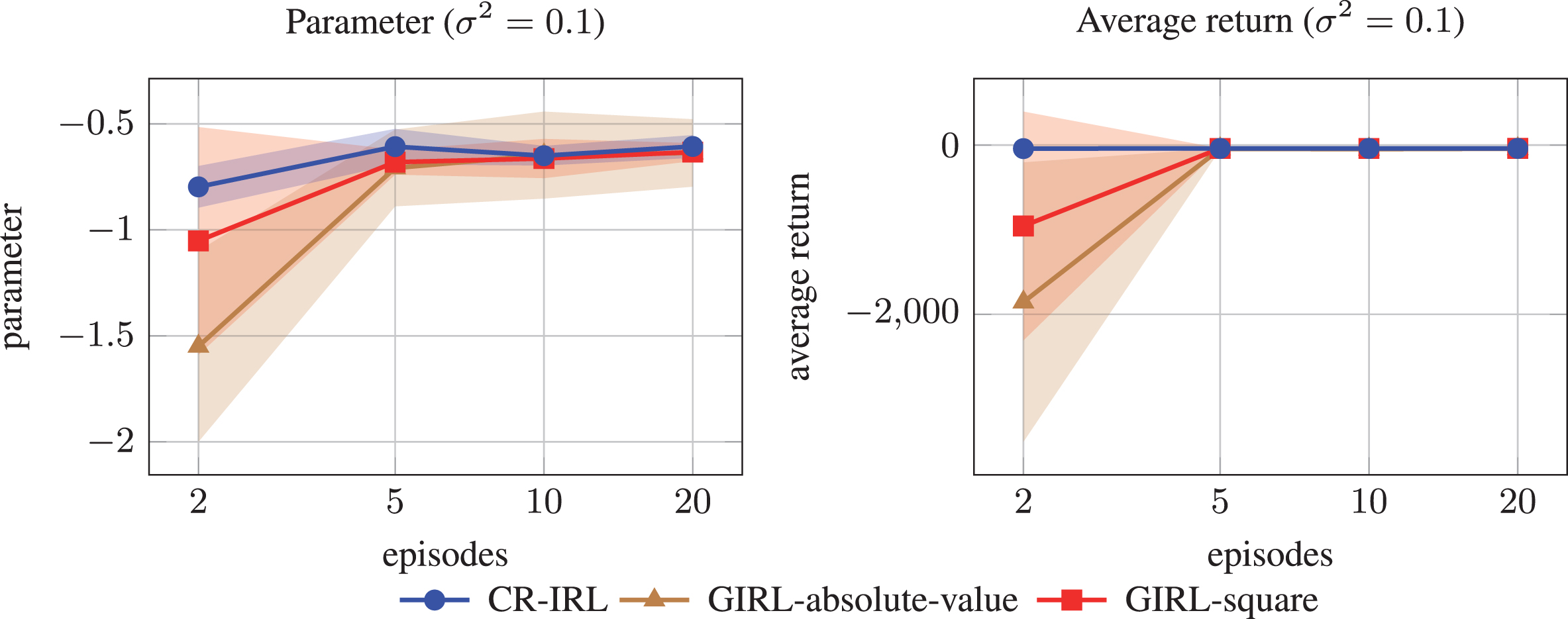
Parameter and average return of 1D-LQG as a function of the number of expert’s trajectories.

Soft penalization. In order to extend the recovered reward function to unseen state-action pairs we adopt a 2NN model with a Gaussian kernel (bandwidth $σ_{S} = σ_{A} = 4$ ). Differently from the discrete case, in the continuous case the penalization must be “soft”, i.e., the more a non-visited state-action pair is far from the visited ones the more it is penalized. The penalized reward function is obtained as a convex combination (α = 0.5) between the non-penalized reward function and a measure of the state-action occupancy: $R^{p} (s, a) = α {\bar{R}}^{np} (s, a) + (1 - α) \bar{p} (s, a),$ where ${\bar{R}}^{np}$ is a scaled version of the recovered reward within the interval [0, 1] and $\bar{p}$ is computed with a “non-normalized” Gaussian kernel KNN approach (bandwidth $σ_{\bar{p}} = 4)$ as: $\begin{matrix} \bar{p} (s, a) & = \frac{\sum_{(s^{'}, a^{'}) \in D_{(s, a)}^{k}} K ((s, a), (s^{'}, a^{'}))}{{max}_{(s^{″}, a^{″}) \in D} \sum_{(s^{'}, a^{'}) \in D_{(s, a)}^{k}} K ((s^{″}, a^{″}), (s^{'}, a^{'}))}, \end{matrix}$ where $D_{(s, a)}^{k}$ is the set of the k closest state-action pairs according to the Euclidean distance and given samples in the dataset $D$ (we use k = 5) and $K$ is a Gaussian kernel. The resulting penalized reward function ranges in the interval [0, 1]. We tested other approaches to perform penalization, such as $R^{p} (s, a) = {\bar{R}}^{np} (s, a) \bar{p} (s, a)$ , no significant difference in performance was detected.

Sensitivity to penalization and number of neighbors. We also investigate the effect of the number of neighbors in the extension of the recovered reward function on unvisited state-action pairs. Figure 13 shows the parameter value and the average return as a function of the number of iterations (the bandwidth of the Gaussian kernel are fixed to $σ_{S} = σ_{A} = 4$ ) and for different values of the expert’s policy variance σ². The KNN interpolation allows reconstructing the reward even in regions of the state-action space that are very far from the region visited by the expert, however, in those regions, the recovered reward is not reliable. We compared the performance of the recovered reward function as is and the performance achieved by penalizing the state-action pairs far from the expert exploration region. In the former case (dashed lines) the convergence is slow and displays a high variance, while in the latter case (solid lines) the learning curve converges faster to the optimal parameter. The number of neighbors has no relevant impact, at least for sufficiently small values, when penalization is applied; while when no penalization is applied the effect is more visible. In particular, when the expert is explorative the recovered reward is smoother (many state-action pairs are visited) so 1NN yields the best performance. As the expert becomes less explorative, a large number of neighbors (50NN) performs better since the recovered reward is more discontinuous. We notice that the penalization becomes more beneficial when the expert’s policy is exploitative (σ² = 0.01).

Fig. 13

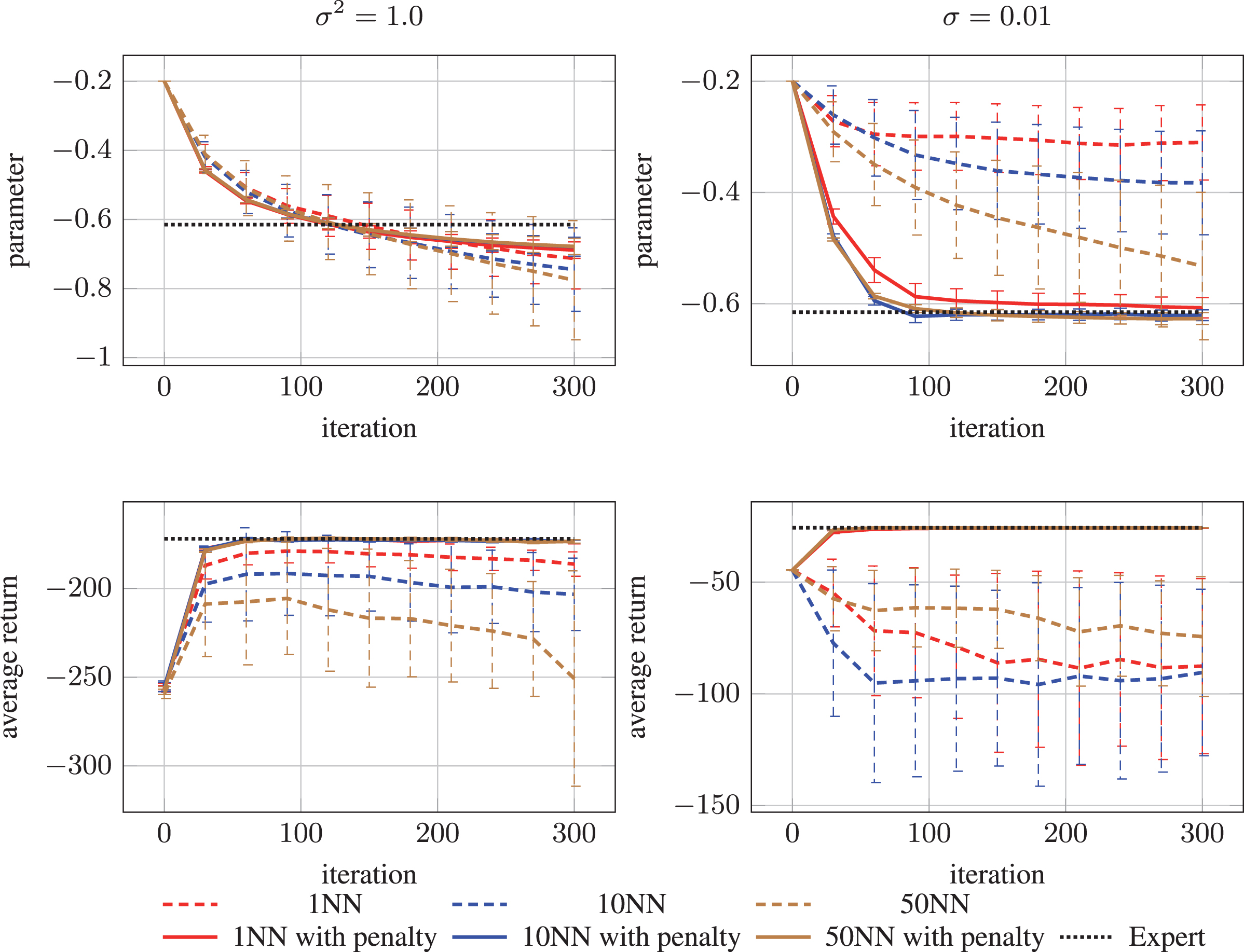
Parameter value and average return of 1D-LQG as a function of the number of iterations of REINFORCE with a different number of neighbors.

Experiments with two-dimensional LQG. In order to compare the second-order criteria we discussed in Section 6, we perform a set of experiments with the two-dimensional LQG (2D-LQG). We consider two settings, as reported in Table 4. In the first case (a) the dynamics of the two states are fully independent, this is equivalent to considering two one-dimensional LQGs running in parallel. In the second case (b), instead, one state influences the other in a symmetric manner; as a consequence, the optimal controller matrix K^* is no longer diagonal. We collect 20 trajectories of length 100 from a Gaussian expert’s policy $N (K^{*} s, Σ$ ), with covariance matrix Σ = 0.01I. We use them to fit via maximum likelihood the parameters (see Table 4 for the ML parameter) of a Gaussian policy: $π_{k, σ^{2}} \sim N (diag (k) s, diag (σ^{2})) .$ (38) Essentially, we restrict our attention to the diagonal control matrices K = diag (k) and we assume that the components of the Gaussian policy are fully uncorrelated Σ = diag (σ ²) =0.01I. Clearly, the optimal Gaussian controller for the case in which the state dynamics are independent falls into this class of policies (a), whereas these policies are not able to represent the optimal controller for the second case (b).

Table 4

Coefficients of the 2D-LQG experiments

Case	A	B	Q	R	λ ²	K ^*	k ^ML
(a)	$(\begin{matrix} 1 & 00 & 1 \end{matrix})$	I	0.9I	0.9I	0.1	$(\begin{matrix} - 0.618 & 00 & - 0.618 \end{matrix})$	$(\begin{matrix} - 0.618 - 0.618 \end{matrix})$
(b)	$(\begin{matrix} 1 & 0.1 0.1 & 1 \end{matrix})$	I	0.9I	0.9I	0.1	$(\begin{matrix} - 0.621 & - 0.083 - 0.083 & - 0.621 \end{matrix})$	$(\begin{matrix} - 0.690 - 0.690 \end{matrix})$

We compare the maximum eigenvalue optimality criterion (ME-opt), the trace optimality criterion (TR-opt) and the trace heuristic (TR-heu). Tables 5 and 6 report the eigenvalues and the trace of the recovered reward functions for cases (a) and (b) respectively. In Fig. 14 the expected return is represented with its second order approximation as a paraboloid in canonical form: $\begin{matrix} J (\tilde{k_{1}} & , \tilde{k_{2}}) \approx J (k_{1}^{ML}, k_{2}^{ML}) \\ + λ_{1} ({\tilde{k_{1}}}^{2} - k_{1}^{ML})^{2} + λ_{2} ({\tilde{k_{2}}}^{2} - k_{2}^{ML})^{2}, \end{matrix}$ where $\tilde{k_{1}}$ and $\tilde{k_{2}}$ correspond to the directions associated to the first and the second eigenvector. Note that the first degree term is missing since $(k_{1}^{ML}, k_{2}^{ML})$ is a stationary point of the expected return.

Table 5

Eigenvalues and trace of the policy Hessian for the recovered reward functions for the 2D-LQGcase (a) (± standard deviation)

Reward function	First eigenvalue	Second eigenvalue	Trace
ME-opt	(-1.34 ± 0.129) e + 4	(-1.34 ± 0.129) e + 4	(-2.68 ± 0.258) e + 4
TR-opt	(-2.72 ± 0.273) e + 4	(-6.66 ± 1.46) e + 3	(-3.40 ± 0.285) e + 4
TR-he	(-1.58 ± 0.171) e + 4	(-7.79 ± 1.13) e + 3	(-2.36 ± 0.249) e + 4

Table 6

Eigenvalues and trace of the policy Hessian for the recovered reward functions for the 2D-LQGcase (b) (± standard deviation)

Reward function	first eigenvalue	second eigenvalue	trace
ME-opt	(-2.79 ± 0.478) e + 4	(-2.18 ± 0.232) e + 4	(-4.97 ± 0.664) e + 4
TR-opt	(-2.94 ± 0.112) e + 5	(-1.58 ± 0.920) e + 3	(-2.96 ± 0.113) e + 5
TR-he	(-1.72 ± 0.134) e + 5	(-7.76 ± 1.50) e + 3	(-1.80 ± 0.146) e + 5

Fig. 14

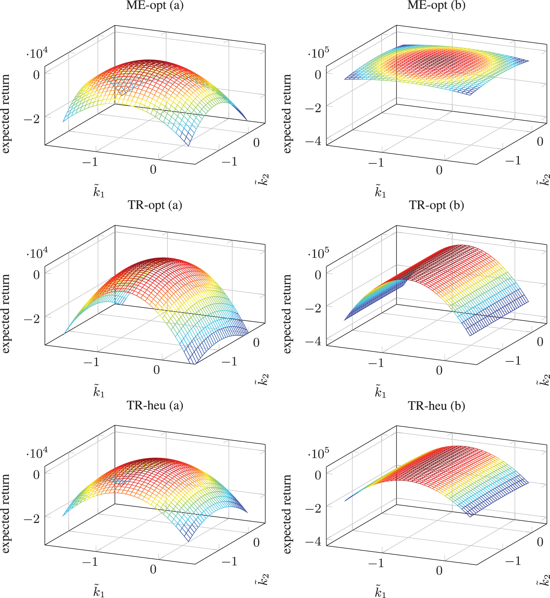
Second order approximation of the expected return for the 2D-LQG.

From Fig. 14 we observe that for case (a) the recovered rewards display a similar shape. This is a consequence of the fact that the two dynamics are independent, therefore the directions of the eigenvectors are not affected one another. On the contrary in case (b), we observe some differences. The ME-opt criterion tends to recover rewards with isotropic shape: the eigenvalues (see Tables 5 and 6) are very close. The TR-opt and the TR-heu, which is its surrogate, tend to sharpen the curve in one direction as much as possible leaving the other direction almost flat.

In terms of learning speed, we observe in Fig. 15 that all the reward functions recovered by CR-IRL allow reaching closely the optimal parameter faster w.r.t. the original reward function. However, in case (a), it is visible that the original reward function converges closer to the optimal parameter. The three criteria, in case (a), do not display significant differences. On the contrary, in case (b), we observe that the reward function recovered by ME-opt displays a better performance w.r.t. the original reward function, converging closer and faster to the optimal parameter. The deviation from the optimal parameter, however, does not have a visible effect on the average return, since all curves in Fig. 16 are almost overlapping.

Fig. 15

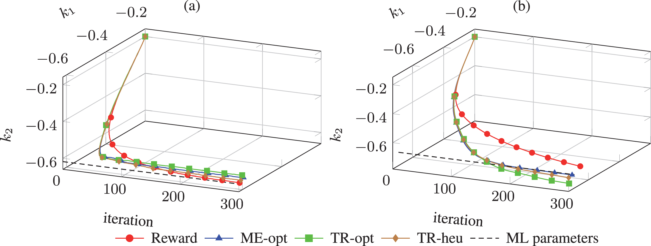
Parameter value for the 2D-LQG as a function of the number of iterations of REINFORCE.

Fig. 16

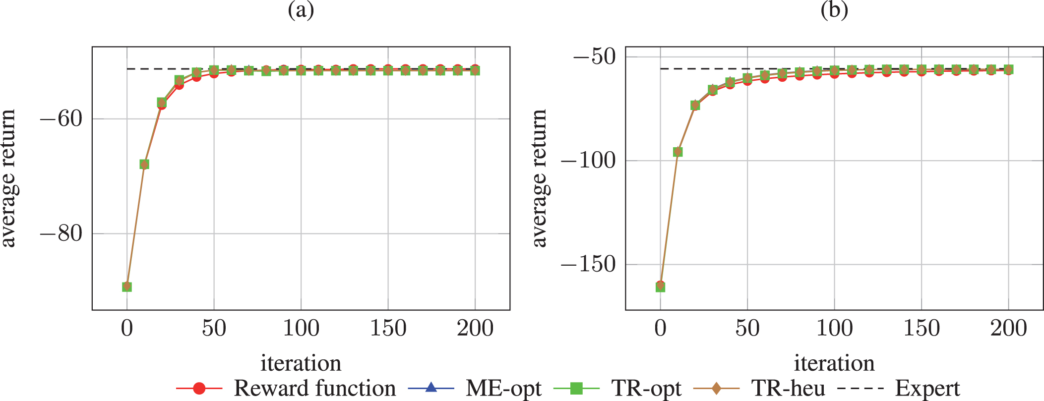
Average return for the 2D-LQG as a function of the number of iterations of REINFORCE.

9.4. Car on the hill.

We further experiment CR-IRL in the continuous Car on the Hill domain [15]. The environment considers a car modeled by a point mass that is traveling on a hill. The action a acts directly on the acceleration of the car. The original formulation assumes to have only two extreme values (full acceleration (a = 4) or full deceleration (a = -4)), but for our convenience, we admit the full range a ∈ [-4, 4]. The control problem objective is roughly to bring the car in a minimum time to the top of the hill while preventing the position p of the car to become smaller than -1 and its speed v to go outside the interval [-3, 3]. Therefore, the state space is continuous of dimension two (the position p and the speed v of the car). If p_t+1 and v_t+1 are such that |p_t+1|>1 or |v_t+1|>3 then a terminal state is reached. The reward function R (p, v, a) is defined through the following expression: $R (p_{t}, v_{t}, a_{t}) = {\begin{matrix} - 1 & if p_{t + 1} < - 1 or | v_{t + 1} | > 3, \\ + 1 & if p_{t + 1} > 1 and | v_{t + 1} | \leq 3, \\ 0 & otherwise . \end{matrix}$ The discount factor γ has been chosen equal to 0.95 and the initial state is p₀ = -0.5 and v₀ = 0. From now on we will indicate with s the pair (p, v).

We approximate the optimal deterministic policy $π_{FQI}^{E}$ via FQI [15] run on 1000 random trajectories, using 50 Extremely Randomized Trees [19] (criterion: mse, min samples split: 5, min samples leaf: 2, iterations: 20). We consider different levels of noisy expert, so that a random action is selected with probability ε ∈ {0, 0.1, 0.2}: $π_{ε}^{E} (a | s) = (1 - ε) π_{FQI}^{E} (a | s) + ε π_{random} (a | s) .$

We exploit N = 20 expert’s trajectories to estimate the parameters w of a Gaussian policy $π_{w} (a | s) \sim N (y_{w} (s), σ^{2})$ , with σ² set to 0.01. The mean y_w (s) is obtained as a radial basis function network [8]: $y_{w} (s) = \sum_{i = 1}^{k} w_{i} e^{- δ | s - s_{i} |^{2}},$ (39) where δ = 0.01 and we consider 40 × 40 centers s_i uniformly distributed in the two-dimensional (position-speed) state space [-4, 4] × [-3, 3]. Notice that this policy allows performing actions in the interval [-4, 4] and not only in {-4, 4}.

Figure 17 shows the original reward function and the reward functions recovered by CR-IRL for the different values of ε. The original reward function displays three regions associated to the reward values +1, 0 and -1. However, most of the +1 region is never reached resulting in penalization when considering the reward functions recovered by CR-IRL. Those functions assign non-zero reward only to the region to which the original reward would assign 0 and to the absorbing state reached as the car gets to the top of the hill with sufficiently small speed. At first glance, the reward functions recovered by CR-IRL are significantly different w.r.t. the original reward and seem not to be informative. Nevertheless, the empirical evaluation demonstrates that they allow computing the optimal policy.

Fig. 17

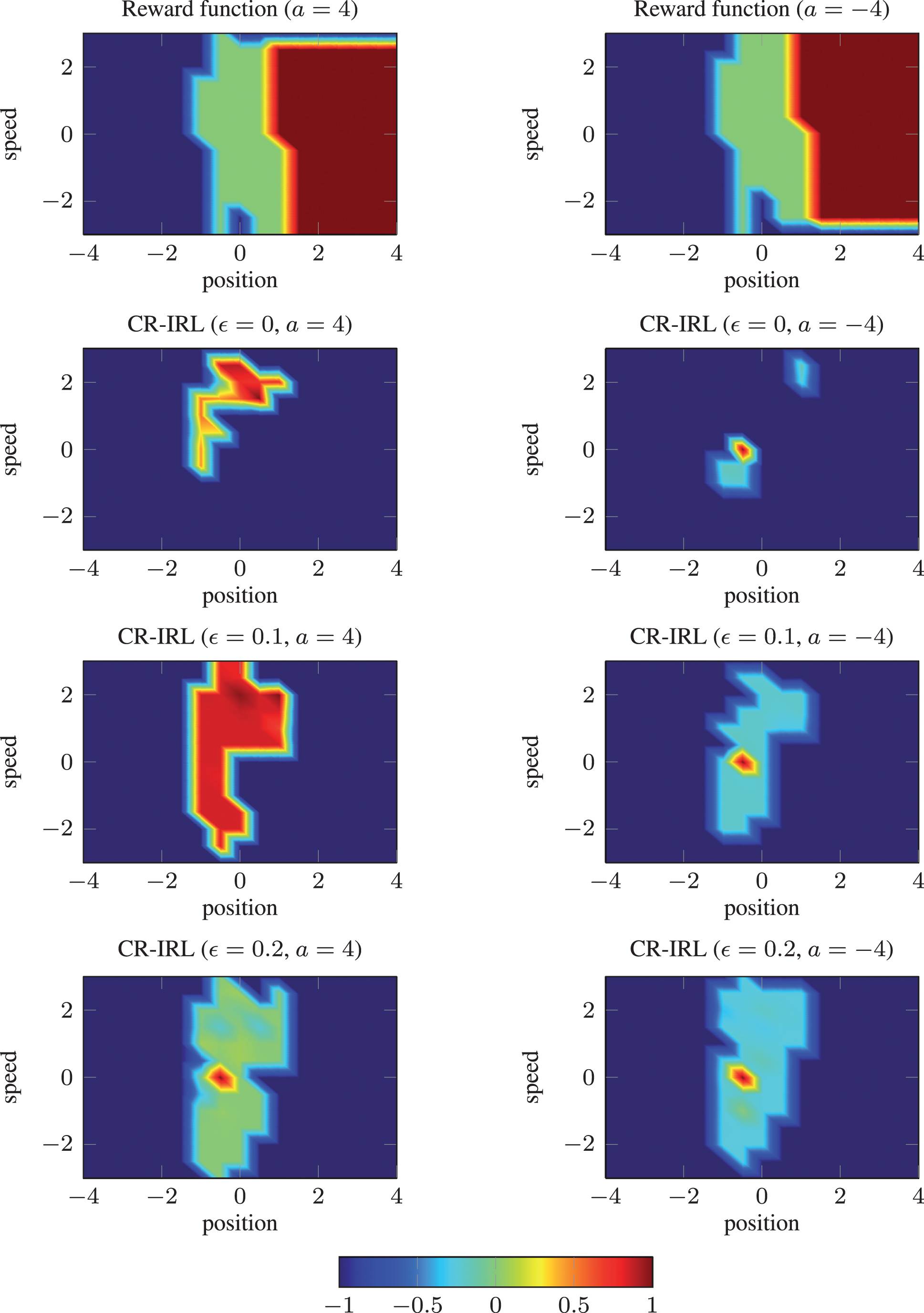
Representation of the recovered reward functions for Car on the Hill.

Learning speed experiments. This experiment is intended to show that the reward function recovered by CR-IRL does not necessarily need to be used with policy gradient approaches. We compare the average return as a function of the number of iterations of FQI, fed with the different recovered rewards.

Figure 18 shows that FQI converges faster to the optimal policy when coped with the reward recovered by CR-IRL rather than with the original reward, regardless of the exploration level ε. When the expert is deterministic (ε = 0), BC reaches the expert’s performance, since the considered class of parametric policies is sufficiently expressive to represent the optimal deterministic policy. Also CR-IRL reaches the expert’s performance in one iteration only.

Fig. 18

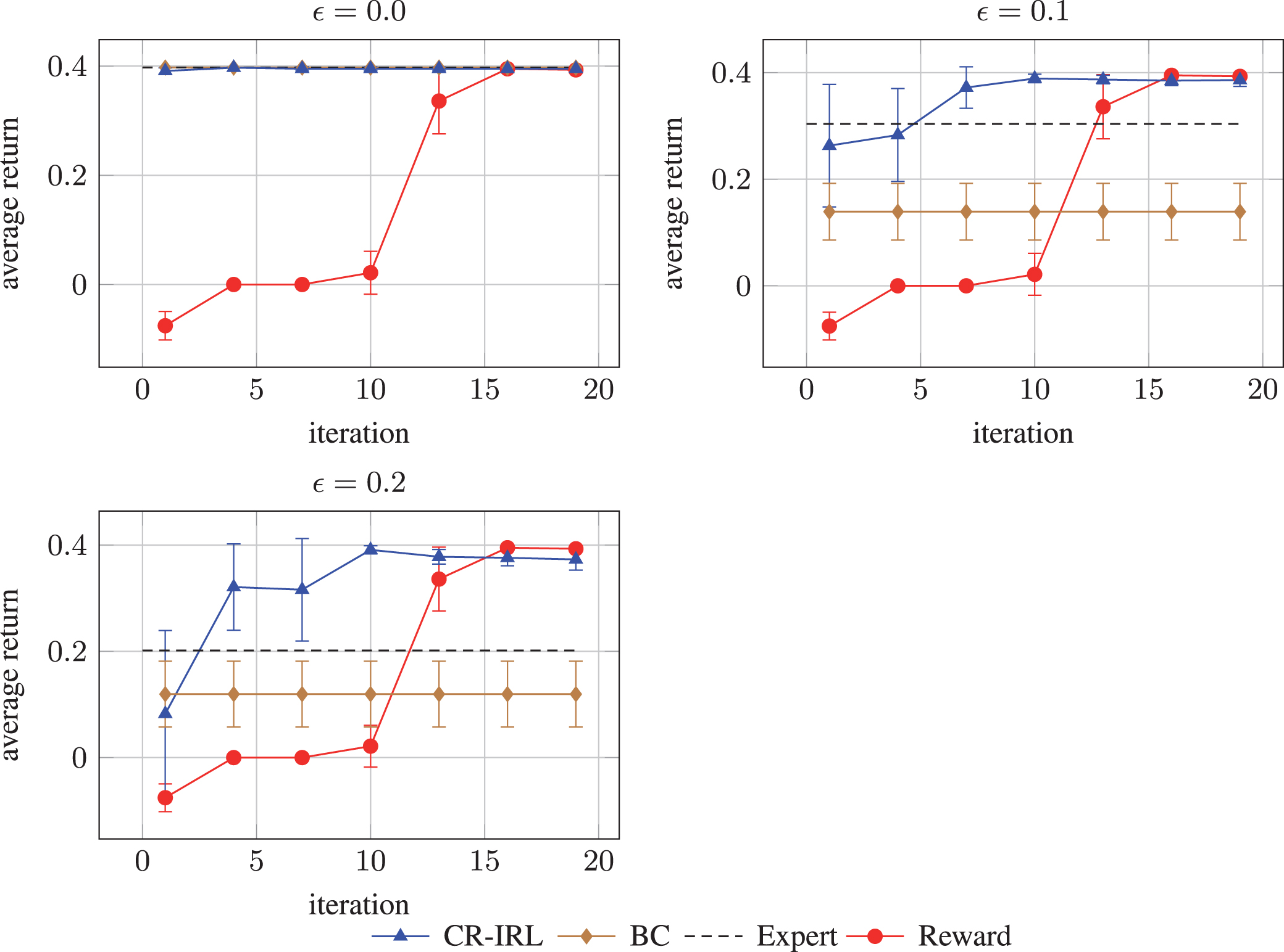
Average return of Car On Hill problem as a function of FQI iterations varying the value of exploration ε.

BC however is not resilient to noise, displaying a significant performance degradation as ε increases. CR-IRL, on the other hand, is able to recover the optimal policy quickly even in the case of explorative experts.

In Fig. 19 we compare the trajectories of the expert’s policy, the maximum likelihood policy (BC) and the policy computed via FQI from the reward recovered by CR-IRL. We can see that when the expert is deterministic the trajectories are almost overlapping. On the contrary, when the exploration rate ε increases we can see that some expert’s trajectories fail to reach the profitable absorbing state. This is a consequence of the fact that a random action is taken with probability ε. BC is almost always able to get the final +1 reward but not optimally in terms of the number of decision epochs required. Finally, CR-IRL, even if trained with a noisy expert, recovers a reward function that induces a policy which is near-optimal, as all trajectories get to the +1 final reward in almost the minimum number of steps.

Fig. 19

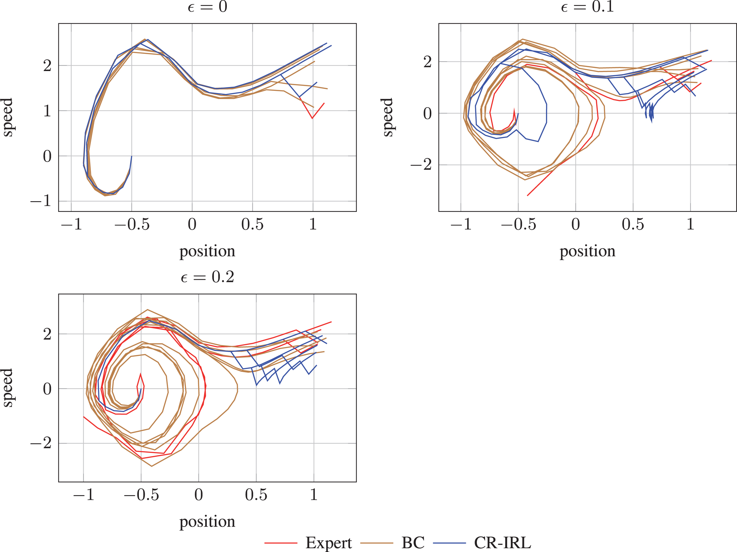
Trajectories of the expert’s policy, the ML policy and the policy computed via FQI from the reward recovered by CR-IRL for different values of ε.

10 Discussion and conclusions

A key step towards enforcing the scalability of IRL to real-world domains is the availability of an algorithm able to construct reward functions requiring just a set of expert’s trajectories. Most of the contributions of this work point to that direction. We presented CR-IRL that mixes BC and IRL in order to construct the features and single out a reward function. BC represents a preliminary step, necessary in order to extract the set of ECO-Q making the gradient vanish. It is worth noting that, for our algorithm, the choice of the policy model is less constraining w.r.t. pure behavioral cloning. Nevertheless, this represents a delicate aspect of CR-IRL, as a poor approximation would make the algorithm extract a suboptimal set of ECO-Q. The main theoretical contributions of this paper lie in the notion of policy rank and in the finite-sample analysis of the feature extraction phase. We think that the informativity of a parametric policy is an appealing notion that, together with Theorem 1, can be used also outside the area of IRL and particularized for specific classes of policies. Once the ECO-Q have been extracted, we proposed two methods to construct the set of ECO-R. Clearly, we focused on the model-free approach that exploits reward shaping in order to build the space of advantage functions. This choice, of course, causes the reduction of the space dimensionality that prevents CR-IRL from considering certain classes of rewards. Nevertheless, using the advantage function as reward function is beneficial for almost all RL algorithms. Finally, we introduced several second-order approaches to select a reward function in the constructed space. The multi-objective interpretation offers a unifying view of the problem, that we particularized for specific choices of optimality criteria, ending in a heuristic that provides good empirical results.

We showed that CR-IRL is able to recover reward functions that can be used to learn optimal policies (in terms of expected return) but at a faster learning rate w.r.t. the original reward function of the problem. Moreover, even though CR-IRL exploits BC to get a parametric representation of the expert’s policy, the policies learned with the reward function recovered by CR-IRL significantly outperform BC. We think this is a key strength of our algorithm, resulting from merging BC and IRL. BC brings to CR-IRL the ability to avoid low-reward regions that the expert has never visited, while IRL, producing a reward representation, allows overcoming the limit of the fixed policy model. Furthermore, CR-IRL outperforms several popular IRL methods designed to recover a reward function as a linear combination of given features, when fed with the set of ECO-R. On the other hand, the performance of the trace heuristic when CR-IRL is fed with automatically generated features, such as Proto-Value Functions, is somehow unsatisfactory. This is a consequence of the fact that the two phases of CR-IRL, feature construction and reward recovery, both originate from conditions on the policy gradient and Hessian and therefore are not independent. The second-order optimality criteria make sense only when the policy gradient is null and take into account only the regions of the environment visited by the expert.

Numerous questions remain open. We believe there is space for further research in this topic, mainly directed towards theoretical and experimental settings. We outline in the followings the main research lines.

10.1 Theoretical analysis of the maximum likelihood policy

CR-IRL, as already seen, requires to estimate a parametric representation of the expert’s policy from the available trajectories. This is a critical point since it requires the choice of a policy model. Although the estimated policy is not used to collect samples, its accuracy might affect the construction of the ECO-Q space and, as a result, the recovered reward function. We have identified two sources of error. First, the maximum likelihood estimation is based on the expert’s trajectories, few trajectories lead to poor approximation even if the expert’s policy falls into the chosen policy space. Second, when the expert’s policy cannot be represented by the policy space, how does the distance between the expert’s policy and the maximum likelihood policy affect the reward construction? In particular, it would be interesting deriving a bound relating the performance gap and the policy distance and study how this error propagates in the policy gradient and for the construction of the set of ECO-Q and ECO-R. We partially answered this question in Section 7.

10.2 Scalability and error propagation

Our approach requires a two-step procedure to build the approximation space for the reward function. As a consequence, this might introduce scalability issues when considering complex environments or large datasets. Indeed, CR-IRL requires to perform two SVDs: one to extract the set of ECO-Q and another for orthogonalizing the set of ECO-R. Furthermore, this contributes to the propagation of the error introduced in the maximum likelihood estimation of the expert’s policy. In order to overcome this limitation, we could resort to trajectory-based formulations of the policy gradient, like (11), in which the reward function appears in place of the Q-function. These equations can be used to build directly the set of ECO-R with no need to pass through the approximation space of the Q-function.

10.3 Reward transferability

The issue of reward transferability is substantial in any real-world application of IRL. This problem has been addressed in a few works and only for simple problems, such as the grid world and the simulated highway driving. In this paper, we have not evaluated the transferability properties of the reward functions recovered by CR-IRL. Intuitively, CR-IRL penalizes deviations from the expert’s policy thus the recovered reward drives the learning process towards the expert’s behavior. Thus it seems that no transferability is enforced by CR-IRL as the agent will tend to reproduce the expert’s policy. Clearly, IRL methods that exploit handcrafted features, encoding implicitly similarities between states and actions, are more suitable to enforce transferability. Nevertheless, if we consider very explorative experts, yielding trajectories in which almost all states and actions are visited, CR-IRL would assign a non-penalized reward even to suboptimal trajectories, producing a more transferable reward.

Appendix

A. Matrix notation for finite Markov decisionprocesses

In this appendix, we report the conventions we adopted for the matrix representation of the finite MDPs. The transition model P is represented as a $| S | | A | \times | S |$ stochastic matrix P, such that: $P_{{sas}^{'}} = P (s^{'} | s, a), \forall s, s^{'} \in S, a \in A .$ The policy of an MDP is represented as a $| S | \times | S | | A |$ matrix π, defined as: $π_{{ss}^{'} a} = {\begin{matrix} π (a | s) & if s^{'} = s \\ 0 & otherwise \end{matrix}, \forall s, s^{'} \in S, a \in A,$ $π = (\begin{matrix} π (a_{1} | s_{1}) & \dots & π (a_{| A |} | s_{1}) & \dots & 0 & \dots & 0 \\ ⋮ & ⋱ & ⋮ & ⋱ & ⋮ & ⋱ & ⋮ \\ 0 & \dots & 0 & \dots & π (a_{1} | s_{| S |}) & \dots & π (a_{| A |} | s_{| S |}) \end{matrix}) .$

The distribution of the initial state is represented by a stochastic vector $μ \in [0, 1]^{| S |}$ . The reward is represented by a vector $r \in ℝ^{| S | | A |}$ . The state value function of policy π is a vector $v^{π} \in ℝ^{| S |}$ , whereas the action value function and the advantage function are vectors $q^{π}, a^{π} \in ℝ^{| S | | A |}$ . Furthermore, we denote with P^π the state transition kernel, i.e., the $| S | \times | S |$ stochastic matrix defined as: $P^{π} = π P .$ We indicate with $r^{π} \in ℝ^{| S |}$ the state reward, defined as: $r^{π} = π r .$ When considering parametric policies π_θ, the gradient of log policies ∇_θ log π_θ are $| S | \times | S | | A | \times k$ tensors. However, for computational reasons they are typically treated as $| S | | A | \times k$ matrices, $\forall a \in A, j = 1, 2, . . ., k$ : $\nabla_{θ} log {π_{θ}}_{saj} = \frac{\partial log π_{θ} (a | s)}{\partial θ_{j}}, \forall s \in S .$

Footnotes

In discounted problems (γ < 1) we can define an “intrinsic horizon”, induced by the discount factor, as $H = \frac{1}{1 - γ}$ .

We want to stress that our primal objective is to recover the reward function since we aim to explain the motivations that guide the expert and, possibly, to transfer it, not just to replicate the behavior. As explained in the introduction, we aim to exploit the synergy between BC and IRL.

Notice that any linear combination of the ECO-Qs also satisfies the first-order optimality condition.

The inner product, as defined, is clearly symmetric, positive definite and linear, but there could be state-action pairs never visited, i.e., $d_{μ}^{π_{θ}} (s, a) = 0$ , making 〈f, f〉_{μ,π_θ} = 0 for non-identically-zero f. To ensure the properties of the inner product, we assume to compute it on visited state-action pairs only.

For a more detailed view of the matrix notation for MDPs refer to Appendix A.

A normalization condition is necessary since the magnitude of the trace of a matrix can be arbitrarily changed by multiplying the matrix by a constant.

This assumption does not allow to consider deterministic policies as G would be infinite. Nevertheless, it is typically used for the analysis of policy gradient methods [60].

Parameter distance is not always a good metric, in particular in presence of parameters that do not affect the policy performance. We will use it for the LQG case only.

We made the choice to use ε-Boltzmann instead of Boltzmann policy since we can leverage on ε to control the exploration-exploitation trade off explicitly.

The maximum eigenvalue optimality criterion is not suitable for this case due to the presence of blocked-to-zero eigenvalues.

When using linear feature models for the policy, zero initialization does not prevent learning, differently from the case of deep neural networks.

References

Abbeel

, Ng.

A.Y.

, Apprenticeship learning via inverse reinforcement learning. In ICML, (2004), p. 1. ACM.

Argall

B.D.

, Chernova

, Veloso

and Browning

, A survey of robot learning from demonstration, Robotics and Autonomous Systems 57(5) (2009), 469–483.

Audiffren

, Valko

, Lazaric

, Ghavamzadeh.

, Maximum entropy semi-supervised inverse reinforcement learning. In IJCAI, (2015), pp. 3315–3321. AAAI Press.

L.C. Baird I. I. I. Advantage updating. Technical report, DTIC Document, 1993.

Bassett

, Deride.

, Maximum a posteriori estimators as a limit of bayes estimators, Mathematical Programming, (2016), pp. 1–16.

Bellman.

, A markovian decision process, Indiana University Mathematics Journal 6 (1957), 679–684.

Ben-Israel

, NE

, Generalized inverses: theory and applications, volume 15. Springer Science & Business Media, 2003.

Bishop.

C.M.

, Pattern recognition, Machine Learning 128 (2006), 1–58.

Böhmer

, Grünewälder

, Shen

, Musial

and Obermayer.

, Construction of approximation spaces for reinforcement learning, Journal of Machine Learning Research 14(1) (2013), 2067–2118.

10.

Boularias

, Kober

, Peters.

, Relative entropy inverse reinforcement learning. In AISTATS, (2011), pp. 182–189.

11.

Cover

T.M.

, Thomas.

J.A.

, Elements of information theory. John Wiley & Sons, 2012.

12.

Cramér

, Mathematical methods of statistics (PMS-9), volume 9. Princeton university press, 2016.

13.

Dietterich.

T.G.

, Hierarchical reinforcement learning with the maxq value function decomposition, Journal of Artificial Intelligence Research 13 (2000), 227–303.

14.

Dorato

, Cerone

, Abdallah.

, Linear Quadratic Control: An Introduction. Krieger Publishing Co., Inc., Melbourne, FL, USA, 2000.

15.

Ernst

, Pierre Geurts and Louis Wehenkel. Treebased batch mode reinforcement learning, Journal of Machine Learning Research 6(Apr) (2005), 503–556.

16.

Finn

, Levine

, Abbeel.

, Guided cost learning: Deep inverse optimal control via policy optimization. In ICML, volume 48 of JMLR Workshop and Conference Proceedings, pp. 49–58. JMLR.org, 2016.

17.

, Luo

, Levine.

, Learning robust rewards with adversarial inverse reinforcement learning, CoRR, abs/1710.11248, 2017.

18.

Furmston

, Barber.

, A unifying perspective of parametric policy search methods for markov decision processes. In NIPS, pp. 2717–2725, 2012.

19.

Geurts

, Ernst

and Wehenkel.

, Extremely randomized trees, Machine learning 63(1) (2006), 3–42.

20.

Goodfellow

, Pouget-Abadie

, Mirza

, Xu

, Warde-Farley

, Ozair

, Courville

, Bengio.

, Generative adversarial nets. In NIPS, (2014), pp. 2672–2680.

21.

Hester

, Vecerik

, Pietquin

, Lanctot

, Schaul

, Piot

, Sendonaris

, Dulac-Arnold

, Osband

, Agapiou

, Leibo

J.Z.

, Gruslys.

, Learning from demonstrations for real world reinforcement learning, CoRR, abs/1704.03732, 2017.

22.

, Ermon.

, Generative adversarial imitation learning, In NIPS, (2016), pp. 4565–4573.

23.

, Gupta

J.K.

, Ermon.

, Modelfree imitation learning with policy optimization. In ICML, volume 48 of JMLR Workshop and Conference Proceedings, (2016), pp. 2760–2769. JMLR.org.

24.

Hwang

C.-L.

, Masud.

A.S.M.

, Multiple objective decision making-methods and applications: a state-of-the-art survey, volume 164. Springer Science & Business Media, 2012.

25.

Kakade.

, A natural policy gradient. In NIPS, pp. 1531–1538. MIT; 1998, 2002.

26.

Kingma

D.P.

, Adam.

J.B.

, A method for stochastic optimization. CoRR, abs/1412.6980, 2014.

27.

Klein

, Geist

, Piot

, Pietquin.

, Inverse reinforcement learning through structured classification. In NIPS, (2012), pp. 1007–1015.

28.

Klein

, Piot

, Geist

, Pietquin.

, A cascaded supervised learning approach to inverse reinforcement learning. In ECML/PKDD (1), volume 8188 of Lecture Notes in Computer Science, (2013), pp. 1–16. Springer.

29.

Levine

, Popovic

, Koltun.

, Feature construction for inverse reinforcement learning. In NIPS, (2010), pp. 1342–1350. Curran Associates, Inc.

30.

Mahadevan.

, Proto-value functions: Developmental reinforcement learning. In ICML, (2005), pp. 553–560. ACM.

31.

Mahadevan

and Maggioni.

, Proto-value functions: A laplacian framework for learning representation and control in markov decision processes, Journal of Machine Learning Research 8(Oct) (2007), 2169–2231.

32.

Mahadevan

, Maggioni

, Ferguson

and Osentoski.

, Learning representation and control in continuous markov decision processes. In, AAAI 6 (2006), pp. 1194–1199.

33.

Manganini

, Pirotta

, Restelli

, Bascetta.

, Following newton direction in policy gradient with parameter exploration. In IJCNN, (2015), pp. 1–8. IEEE.

34.

Mengi

, Yildirim

E.A.

and Kilic.

, Numerical optimization of eigenvalues of hermitian matrix functions, SIAM Journal on Matrix Analysis and Applications 35(2) (2014), 699–724.

35.

Metelli.

A.M.

, Compatible reward inverse reinforcement learning. Master’s thesis, Politecnico di Milano, 2017. http://hdl.handle.net/10589/135141.

36.

Metelli

A.M.

, Pirotta

, Restelli.

, Compatible reward inverse reinforcement learning. In NIPS, (2017), pp. 2050–2059.

37.

Neu

, Szepesvári

, Training parsers by inverse reinforcement learning, Machine Learning, 77(2-3) (2009), 303–337.

38.

A.Y.

, Harada

and Russell.

, Policy invariance under reward transformations: Theory and application to reward shaping. In , ICML 99 (1999), pp. 278–287.

39.

A.Y.

, Russell

S.J.

, et al., Algorithms for inverse reinforcement learning. In ICML, (2000), pp. 663–670.

40.

Nocedal

, Wright.

S.J.

, Numerical Optimization. Springer Series in Operations Research and Financial Engineering. Springer New York, 2006.

41.

Overton.

M.L.

, On minimizing the maximum eigenvalue of a symmetric matrix, SIAM Journal on Matrix Analysis and Applications 9(2) (1988), 256–268.

42.

Parisi

, Pirotta

and Restelli.

, Multiobjective reinforcement learning through continuous pareto manifold approximation, Journal Artificial Intelligence Research 57 (2016), 187–227.

43.

Peters

and Schaal.

, Reinforcement learning of motor skills with policy gradients, Neural networks 21(4) (2008), 682–697.

44.

Piot

, Geist

, Pietquin.

, Boosted and reward-regularized classification for apprenticeship learning. In AAMAS, (2014), pp. 1249–1256. IFAAMAS/ACM.

45.

Pirotta

, Restelli.

, Inverse reinforcement learning through policy gradient minimization. In AAAI, (2016), pp. 1993–1999.

46.

Puterman.

M.L.

, Markov decision processes: Discrete stochastic dynamic programming. 1994.

47.

Ratliff

N.D.

, Bagnell

J.A.

, Zinkevich.

, Maximum margin planning. In ICML, volume 148 of ACM International Conference Proceeding Series, (2006), pp. 729–736. ACM.

48.

Ratliff

N.D.

, Silver

and Bagnell.

J.A.

, Learning to search: Functional gradient techniques for imitation learning, Autonomous Robots 27(1) (2009), 25–53.

49.

Sutton

R.S.

, Barto.

A.G.

, Reinforcement learning: An introduction, volume 1. MIT press Cambridge, 1998.

50.

Sutton

R.S.

, McAllester

D.A.

, Singh

S.P.

, Mansour.

, Policy gradient methods for reinforcement learning with function approximation. In NIPS, (1999), pp. 1057–1063. The MIT Press.

51.

Sutton

R.S.

, McAllester

D.A.

, Singh

S.P.

, Mansour

and Policy

et al.

, gradient methods for reinforcement learning with function approximation. In, NIPS 99 (1999), pp. 1057–1063.

52.

Syed

, Bowling

M.H.

, Schapire.

R.E.

, Apprenticeship learning using linear programming. In ICML, volume 307 of ACM International Conference Proceeding Series, (2008), pp. 1032–1039. ACM.

53.

Syed

, Schapire.

R.E.

, A game-theoretic approach to apprenticeship learning. In NIPS, (2007), pp. 1449–1456.

54.

Tateo

, Pirotta

, Restelli

, Bonarini.

, Gradient-based minimization for multi-expert inverse reinforcement learning. In Computational Intelligence (SSCI), 2017 IEEE Symposium Series on, (2017), pp. 1–8. IEEE.

55.

Todorov.

, Efficient computation of optimal actions, Proceedings of the national academy of sciences 106(28) (2009), 11478–11483.

56.

Uchibe.

, Model-free deep inverse reinforcement learning by logistic regression, 891– , Neural Processing Letters 47(3) (2018), 905.

57.

Vidal

J.M.

, Vidal.

J.M.

, Fundamentals of multiagent systems. 2006.

58.

Weissman

, Ordentlich

, Seroussi

, Verdu

, Weinberger.

M.J.

, Inequalities for the l1 deviation of the empirical distribution, Hewlett-Packard Labs, Tech. Rep, (2003).

59.

Williams.

R.J.

, Simple statistical gradient-following algorithms for connectionist reinforcement learning, Machine learning 8(3-4) (1992), 229–256.

60.

Zhao

, Hachiya

, Niu

, Sugiyama.

, Analysis and improvement of policy gradient estimation. In NIPS, (2011), pp. 262–270.

61.

Ziebart.

B.D.

, Modeling purposeful adaptive behavior with the principle of maximum causal entropy. 2010.

62.

Ziebart

B.D.

, Maas

A.L.

, Bagnell

J.A.

, Dey.

A.K.

, Maximum entropy inverse reinforcement learning. In AAAI, 8 (2008), pp. 1433–1438. Chicago, IL, USA.