Exploiting auto-encoders for explaining black-box classifiers

Abstract

Recent years have witnessed the rise of accurate but obscure classification models that hide the logic of their internal decision processes. In this paper, we present a framework to locally explain any type of black-box classifiers working on any data type through a rule-based model. In the literature already exists local explanation approaches able to accomplish this task. However, they suffer from a significant limitation that implies representing data as a binary vectors and constraining the local surrogate model to be trained on synthetic instances that are not representative of the real world. We overcome these deficiencies by using autoencoder-based approaches. The proposed framework first allows to generate synthetic instances in the latent feature space and learn a latent decision tree classifier. After that, it selects and decodes the synthetic instances respecting local decision rules. Independently from the data type under analysis, such synthetic instances belonging to different classes can unveil the reasons for the classification. Also, depending on the data type, they can be exploited to provide the most useful kind of explanation. Experiments show that the proposed framework advances the state-of-the-art towards a comprehensive and widely usable approach that is able to successfully guarantee various properties besides interpretability.

Keywords

Explainable artificial intelligence auto-encoders interpretable machine learning model-agnostic explainer data-agnostic explainer

1 Introduction

Explaining the decisions of black-box classifiers is one of the the principal obstacles to the acceptance and trust of applications based on Artificial Intelligence (AI) [37, 44]. Magazines and newspapers are full of commentaries about AI systems taking critical decisions that heavily impact our life and society, from pedestrian detection in self-driving cars to loan concession in bank systems. The problem is not only due to the increasing automation of AI decision-making, but mostly to the fact that the underlying algorithms are opaque and their logic unexplained [48]. The main cause for this lack of transparency is that the procedures for inferring a decision model from data cannot be entirely controlled due to their complexity that is too high for humans [18]. On the one hand, the EU defines new regulations requiring that automated decisions should be explained 1 while, on the other hand, more and more complex and not understandable models for decision-making are designed [42, 49]. The lack of transparency in machine learning models used by AI systems grants them the power to perpetuate forms of injustice by learning bad habits from the data: if the training data contains biased decision instances, the resulting model inherits the biases and recommends discriminatory or simply wrong decisions [8, 46].

As a consequence, there has recently been a booming of proposals for explaining machine learning classifiers [27, 37]. Researchers are mainly focusing on post-hoc explainers aimed at unveiling the reasons for a black-box classifier. A wide array of post-hoc approaches have been proposed ranging from global approaches explaining the whole decision logic of a classifier to local approaches explaining the decision of a specific input instance. Another categorization involves model-agnostic approaches that assume no information on the classifier, vs. model-specific approaches that only work on classifiers of a specific type. A radically different direction aims at developing new classifiers that are interpretable by-design [52].

The objective of this paper is to define a local model-agnostic and data-agnostic explanation framework to explain the decisions taken by obscure black-box classifiers on specific input instances. Therefore, our proposal would not be tied to a specific type of data or a specific type of classifier. In the literature, approaches with these characteristics, such as lime [51], have already been proposed. Such approaches generate a local synthetic neighborhood around the instance to explain and mime the behavior of the black-box classifier using an interpretable decision model trained on the neighborhood. However, the existing local model-agnostic and data-agnostic explainers exhibit drawbacks that may negatively impact their reliability.

First, they do not consider existing relationships between features of the data during the neighborhood generation. Second, the user has to specify the number of components of an explanation. Third, and most importantly, the synthetic neighborhood generation does not produce “meaningful” instances because it only works by obscuring/suppressing the actual values. For instance, for images, lime replaces randomly selected areas of the image to explain with a fixed color, typically black or white [51]. We highlight that the final explanation can completely change depending on the color adopted. Similarly, lime for text, uses as local synthetic instances text from which randomly selected words are simply removed from the input [51]. In [54], lime is used to explain time series classifiers, and the synthetic time series in the neighborhood are generated by replacing sub-parts of the time series under analysis with a fixed value (e.g., the mean). Therefore, in all these cases, the local synthetic instances consist of an altered input with some obscured parts without any guarantee of training the interpretable model on plausible synthetic instances. On the other hand, when lime is applied on tabular data, the features are replaced with values randomly selected from a uniform or Gaussian distribution hence resulting in reliable synthetic instances. Our objective is to provide meaningful explanations of the decisions returned independently from the data type and having an explanation that is based on formal logic which should be as close as possible to the language of reasoning.

We propose llore , a Latent LOcal Rule-based Explainer based on lore [25]. llore is a local, post-hoc, model-agnostic, and data-agnostic explanation framework able to overcome the limitations of existing approaches by exploiting the latent feature space, learned through different types of auto-encoders [31 , 41] for the neighborhood generation process. Given an instance of any type classified by a black-box, llore allows instantiating a data-specific explainer following the explanation framework structure. The explainer will be able to return a meaningful explanation for the classification reasons. First, it generates synthetic instances in the latent feature space using a pre-trained autoencoder. Then, it learns a latent decision tree classifier. After that, it selects and decodes the synthetic instances respecting local decision rules observed on the decision tree. Finally, independently from the data type, it returns an explanation that always consists of a set of exemplars and counter-exemplars synthetic instances illustrating, respectively, instances classified with the same label and with a different label than the instance to explain, which may be visually analyzed to understand the reasons for the classification. Additionally, a data-specific explanation can be built on the exemplars and counter-exemplars.

We instantiated llore for images [26], time series [28] and text [35] realizing ad-hoc logic-based explanations. A wide experimentation on datasets of different types and explaining different black-box classifiers empirically demonstrate that llore -based explainers overtakes existing explanation methods providing meaningful, stable, useful, and really understandable explanations.

The rest of the paper is organized as follows. Section 2 discusses related works. Section 3 introduces basic concepts for presenting the explanation framework, which is described in Section 4. Section 5 presents the experiments. Finally, Section 6 summarizes our contribution, its limitations, and future work.

2 Related works

The research of methods for explaining black-box decision systems has recently caught much attention [1 , 45]. The aim is to couple effective machine learning classifiers with explainers of their logic. Explanation methods can be categorized with respect to three aspects [27]. One contrasts model-specific vs model-agnostic approaches, depending on whether the explanation method exploits knowledge about the internals of the black-box or not. The other contrasts local vs global approaches, depending on whether the explanation is provided for any specific instance or for the logic of the black-box as a whole. Finally, the last contrast data-specific vs data-agnostic approaches, depending on whether the explanation method is designed to work on a specific data type or not. The proposed explanation framework llore fits the line of research of local, model-agnostic and data-agnostic methods originated with [51] and extended in several directions in the last few years.

lime [51] randomly generates instances “around” the instance to explain creating a local neighborhood. Then, it learns a linear regressor on the neighborhood instances labeled with the black-box decision, and it returns as an explanation the feature importance of the most relevant features in the linear model. The number of such features has to be specified by the user. This can be a limitation since users may have no clue about the correct number of features. Explanations in forms of feature importance are also produced by shap and maple . shap [40] connects game theory with local explanations and overcomes the lime limitation related to the user-provided number of features. shap exploits the Shapely values of a conditional expectation function of the black-box by providing the unique additive feature importance. maple [50] provides explanations as features importance of a linear model by exploiting random forests for the supervised selection of the features. Unfortunately, the approaches above base their explanation on features’ importance, but, as humans, we generally prefer explanations in a logical form such as of rules [34, 60]. In [25] we overcame these deficiencies by presenting lore , a local rule-based explainer for tabular data that returns as explanation factual and counter-factual rules.

Besides being model-agnostic, lime is also data-agnostic. However, it employs conceptually different neighborhood generation strategies [24] for tabular data, images, and texts. For images, lime randomly replaces actual super-pixels with super-pixels containing a fixed color. For texts, it randomly removes words. Thus, both for images and text lime “suppresses” parts of the actual information in the data. On the other hand, for tabular data, lime assumes uniform distributions for categorical attributes and normal distributions for the continuous ones. Such limitations prevent lime from basing the local regressor used to extract the explanation on meaningful synthetic instances. Similarly, in [54] lime is used to explain time series classifiers. In this case, randomly selected parts of the time series under analysis are replaced with fixed values to generate the synthetic time series for the neighborhood. Similar problems affects also shap and maple . Our proposed explanation framework allows overcoming these limitations by guaranteeing comparable synthetic data generation among all the different data types, ensuring meaningful synthetic instances to learn interpretable local surrogate models.

3 Setting the stage

In this paper we address the black-box outcome explanation problem [27]. A classification dataset X, Y consists of a set X = {x₁, x₂, …, x_n} instances with l labels (or classes) assigned to each instances in the vector $Y \in ℕ^{n}$ . As data types we consider tabular records, images, time series, and text [23]. A tabular record $x \in ℝ^{m}$ , i.e., a set of m attribute-value pairs x = {(a₁, v₁) , …, (a_m, v_m)} where each a_i is an attribute and v_i is a value of the domain of a_i. An image x is a m × q matrix where each element x_i,j ∈ [0, 255] represents a pixel value. A time series is an ordered set of m real-valued variables x = {t₁, …, t_m}, i.e., $t_{i} \in ℝ$ . A text is an ordered set of u items x = {w₁, …, w_u}, where w_i represents a word.

Given a black-box classifier b and an instance x classified by b, i.e., b (x) = y, our aim is to provide an explanation e for the decision b (x) = y. We use the notation b (X) = Y as a shorthand for {b (x) | x ∈ X} = Y. We assume that b can be queried at will. More formally, we aim to address the following problem:

Definition 1. Let b be a not interpretable classifier, and x an instance whose decision y = b (x) has to be explained, the black-box outcome explanation problem consists in finding an explanation e ∈ E belonging to a human-interpretable domain E.

In order to keep our paper self-contained, we summarize the following concepts necessary to comprehend the proposed explanation framework.

3.1 Local rule-based explanation

Widely adopted human-interpretable domain E consists of instance-based explanations and if-then rules [10]. Instance-based explanations rely on examples highlighting the crucial traits characterizing the decision. On the other hand, if-then rules provide conditions met by the instance x to be explained that determined the answer of the black-box. Rules can also be used to provide counter-factuals, namely alternative conditions, not met by x, that would determine a different answer by the black-box [13]. In our approach, we will build on lore [25], a local explainer for tabular data that learns a local decision tree from a given neighborhood Z of the instance to explain. Such a tree is a surrogate model of the black-box, i.e., it is trained to reproduce the decisions of the black-box. lore provides in output: (i) a factual rule r, corresponding to the path in the local surrogate tree that explains why x has been labeled as y by b, and (ii) a set of counterfactual rules Φ, explaining which changes in x would invert the class y assigned by b. lore learns on the synthetic neighborhood Z of x an interpretable local decision tree that reproduces the behavior of b. The neighborhood Z is generated through a genetic algorithm to account for instances similar to x and with the same label, i.e., y = b (x), and for instances similar to x but with a different label, i.e., y ≠ b (x). The local explanation, including factual and counterfactual rules, is derived from the tree’s structure.

3.2 Auto-encoders

In an explanation process, it is crucial to respect the distributions of actual data in synthetically generated examples created for studying the black-box behavior in the neighborhood of the instance to explain. We ensure this property by using auto-encoders (AE) [31]. An AE is a neural network trained to learn a representation that reduces the dimensionality from m to k and captures non-linear relationships. An encoder $ζ : ℝ^{m} \to ℝ^{k}$ , and a decoder decoder $η : ℝ^{k} \to ℝ^{m}$ are simultaneously learned with the objective of minimizing the reconstruction loss. Starting from the encoding z = ζ (x), the autoencoder tries to reconstruct a representation as close as possible to its original input $x ≃ \tilde{x} = η (z)$ . After the learning, the decoder can be used to reconstruct instances never observed, aiming to be used as a generative model. In the literature, there exist several variants designed to guarantee valuable properties on the learned representations, such as Generative Adversarial Network (GAN) [21], Variational Auto-Encoders (VAE) [33], and Adversarial Auto-Encoders (AAE) [41].

AAEs are regularized by matching the aggregated posterior distribution of the latent representation of the input data to an arbitrary prior distribution through the usage of a discriminator $θ : ℝ^{k} \to [0, 1]$ that establish if the latent instance z comes from the actual probability distribution. Indeed, the AAE learning involves two phases: the reconstruction aimed at training the encoder and decoder to minimize the reconstruction loss; the regularization aimed at training the discriminator using training data and encoded values. The discriminator θ ensures that the reconstructed instances are meaningful ones. On the other hand, the difference between VAE and AE is that VAEs are trained by considering an additional limitation on the loss function such that the latent space is scattered and does not contain “dead zones”. Indeed, the name variational comes from the fact that VAEs work by approaching the posterior distribution with a variational distribution. The encoder ζ emits the parameters for this variational distribution in terms of a multi-factorial Gaussian distribution, and the latent representation is taken by sampling this distribution. The decoder η takes as input the latent representation and focuses on reconstructing the original input from it. Avoiding dead zones ensures that the instances reconstructed from vectors in the latent space are meaningful [11].

4 Latent local rule-based explainer

In this section, we describe llore (Latent LOcal Rule-based Explainer), a local post-hoc model-agnostic meta-explainer solving the outcome explanation problem. Given an instance x to explain and a black-box b, llore provides a factual latent rule r, and a set of latent counterfactual rules Φ. Such latent rules can be used to identify in the latent space a set of exemplars and counter-exemplars, i.e., synthetically generated instances classified with the same and with a different outcome than x, respectively. As detailed in the following, exemplars and counter-exemplars can be visually analyzed to understand the reasons for the classification, and also exploited to build other types of explanations. To obtain r and Φ, llore exploit the AE architectures described in Section 3.2 and works as described by the workflow in Figure 1.

Fig. 1

Latent Local Rule-based Explainer. llore takes as input the instance x to explain and the black-box b. With the encoder trained by the AE, VAE or AAE, it turns x into its latent representation z. Then, the neighgen module uses z and b to generate the latent local neighborhood H. The valid instances are decoded in $\tilde{H}$ by the disde module. Instances in $\tilde{H}$ are labeled with the black-box $Y = b (\tilde{H})$ . H and Y are used to learn a decision tree classifier. At last, a latent decision rule r and the latent counter-factual rules Φ for z are returned.

Encoding. Let consider that llore has available a pre-trained AE described by the functions ζ and η representing the encoder and decoder, respectively. First, the instance $x \in ℝ^{m}$ to be explained, independently from its data type but according to the data type treated by the AE, is passed as input to the AE where the encoder ζ returns the latent representation $z \in ℝ^{k}$ using k latent features with k ⪡ m. We underline that the training necessary to obtain sound and reliable encoder and decoder functions is not necessarily trivial and strictly depends on the data type and class distributions. High performance of AEs, and thus of these functions, might impact positively on the explanations returned by llore and, in turn, in the trust transmitted to the final user. However, we assume that the AEs used by llore are well-trained and reliable for data generation. We check and guarantee this assumption empirically by observing the reconstruction error.

Neighborhood Generation. After that, llore generates a set of synthetic instances H in the latent feature space, with characteristics close to those of z using the neighgen (neighborhood generator) function in Figure 1. Several reasons exist to prefer the generation of a synthetic neighborhood around z in the latent domain instead of around x in the real domain. First, the AEs allow to apply the same algorithm for the neighborhood generation independently for the data type. Second, the latent space has a dimensionality lower than the original one, providing both speed-up and a higher quality guarantee in the usage of approaches that could suffer from dimensionality. Finally, depending on the type of AE adopted, the variation of a latent feature might cause the simultaneous variation of multiple real features among which certain relationships exist. On the other hand, an independent mutation in the real domain would not account for such relationships. Since the goal is to learn a latent surrogate model predictor on H able to simulate the local decision behavior of b, H must include instances with both decision outcomes, namely H = H₌ ∪ H_≠ where instances h ∈ H₌ are such that $b (\tilde{h}) = b (x)$ , and h ∈ H_≠ are such that $b (\tilde{h}) \neq b (x)$ . We name $\tilde{h} \in ℝ^{m}$ the decoded version of an instance $h \in ℝ^{k}$ in the latent feature space. The neighborhood generation of H may be accomplished using different strategies ranging from pure random strategy [24, 51] using a given distribution, to a genetic approach which generates h ∈ H₌ ∪ H_≠ by maximizing a fitness function like in [25]. After the generation process, for any instance h ∈ H, llore exploits a discriminator and decoder module (disde) that applies the decoder η to instances in H returning $\tilde{H}$ , i.e., $\tilde{H} = η (H)$ . In case the AE is an AAE, then the disde module applies η only on the latent features which resemble real ones according to the discriminator θ of the AAE (see Section 3.2). Then, llore queries b with $\tilde{H}$ to get the class Y of the synthetic instances, i.e., $b (\tilde{H}) = Y$ . We notice that disde returns both $\tilde{H}$ and H: $\tilde{H}$ is used to query the black-box, while H is used to train a local latent model model as described in the next section.

Latent Rules Extraction. At this stage, llore builds a latent decision tree on the instances H labeled with the black-box decision $b (\tilde{H})$ . Such a predictor is intended to locally mimic the behavior of b in the neighborhood H. From the decision tree llore extracts the latent factual rule r and counter-factual rules Φ. llore considers decision tree classifiers because: (i) decision rules can naturally be derived from a root-leaf path in a decision tree; and, (ii) counter-factual rules can be extracted by symbolic reasoning over a decision tree. The premise p of a decision rule r = p → y is the conjunction of the splitting conditions in the nodes of the path from the root to the leaf that is satisfied by the latent representation h of the instance to explain x. For the counter-factual rules Φ, llore selects the closest rules in terms of splitting conditions leading to a label ¬y different from y, i.e., the rules {q → ¬ y} such that q is the conjunction of splitting conditions for a path from the root to the leaf labeling an instance h with ¬y and minimizing the number of splitting conditions falsified with respect to the premise p of r. We highlight that, given an instance x, the corresponding z is covered by a single latent rule r. On the other hand, given an instance x and the rule r that covers z, several different counter-factual rules Φ might exist depending on the tree structure 2 .

Thus, we name this meta-explainer llore as a variant of lore [25] operating in the latent feature space.

Explanation Extraction. The latent rules r and Φ allow to easily select among H, or among other synthetic instances generated through the AE, the latent records respecting the constraints described by r and Φ and which highly characterize the decision boundary in the vicinity of x. Let us indicate with H such latent records. Their reconstruction $η (H) = \tilde{H} = {\tilde{H}}_{=} \cup {\tilde{H}}_{\neq}$ is formed by exemplars ${\tilde{H}}_{=}$ s.t. $b ({\tilde{H}}_{=}) = b (x)$ and counter-exemplars ${\tilde{H}}_{\neq}$ s.t. $b ({\tilde{H}}_{\neq}) \neq b (x)$ in the same domain of x. Exemplars and counter-exemplars form an instance-based explanation highlighting the most similar instances to x obtaining the same decision or a different one and allowing a user to understand which are the discriminatory aspect of the black-box w.r.t. x. Finally, we highlight that, even though not directly used to return the final explanation like in lore , the decision tree is fundamental to identify the exemplars and counter-exemplars and, therefore, to select the instances used to build the various types of explanation discussed in the following with respect to the latent rule and counterfactual rules r and Φ.

In the remainder of this section, we show how instantiations of the meta-explainer llore to images, time series, and text are straightforward, and how we can exploit exemplars and counter-exemplars to build data-specific types of explanations.

4.1 Explaining image classifiers

In [26] we design abele (Adversarial black-box Explainer generating Latent Exemplars), an instantiation of llore to explain image classifiers. As AE, abele adopts an AAE [41] in order to guarantee the plausibility of the latent instances returned by the disde module. Since we are in the image data domain, abele exploits the exemplars to build a saliency map to include as part of the explanation. A saliency map s typically highlights the areas of an image x that mostly contributed to its classification outcome b (x). abele builds the saliency map by exploiting the exemplars by first computing the pixel-to-pixel-difference between x and each exemplar in the set ${\tilde{H}}_{=}$ , and then, it assigns to each pixel of the saliency map s the median value of all differences calculated for that pixel. Thus, formally for each pixel i of the saliency map s we have: $s_{i} = {median}_{\forall \tilde{h} \in {\tilde{H}}_{=}} (x_{i} - {\tilde{h}}_{i})$ Thus, the saliency maps s returned by abele highlights both the areas of x that contribute to its b (x), but also the areas of x that push it towards another class.

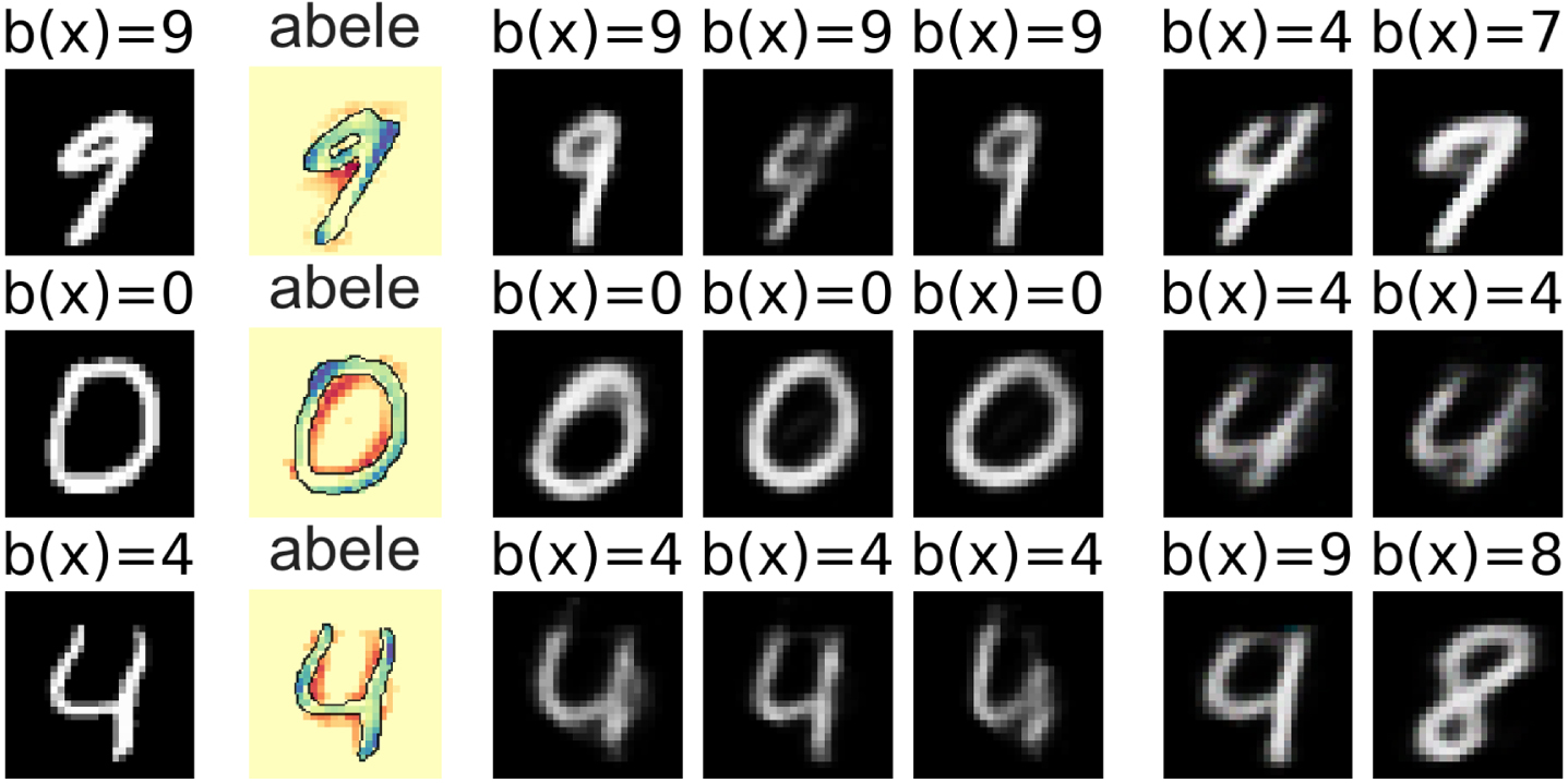
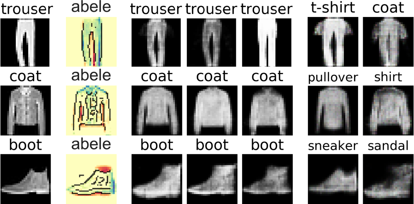
In Figures 2 and 3 we report explanations of a DNN trained on the mnist and fashion datasets 3 https://www.kaggle.com/zalando-research/fashionmnist. The first column contains the image to explain x together with the label provided by the black-box b, while the second column contains the saliency maps provided by abele . We indicate with the yellow color the areas that are common between x and the exemplars ${\tilde{H}}_{=}$ , with the red color the areas contained only in the exemplars, and with the blue color the areas contained only in x. This means that yellow areas must remain unchanged to obtain the same label b (x), while red and blue areas can change without impacting the black-box decision. In particular, with respect to x, an image obtaining the same label can be darker in blue areas and lighter in red areas. In other words, blue and red areas express the boundaries that can be varied, and for which the class remains unchanged.

Fig. 2

abele explanations for mnist.

Fig. 3

abele explanations for fashion.

For example, with this type of saliency map we can understand that a nine may have a more compact circle, a zero may be more inclined, a coat may have no space between the sleeves and the body, and that a boot may have a higher neck. Moreover, we can notice how, besides the background, there are some “essential” yellow areas within the main figure that can not be different from x: e.g. the leg of the nine, the crossed lines of the four, the space between the two trousers. Besides, for each instance we show three exemplars and two counter-exemplars. Observing these images we can notice how the label nine is assigned to images very close to a four, but until the upper part of the circle remains connected, it is still classified as a nine. On the other hand, looking at counter-exemplars, if the upper part of the circle has a hole or the lower part is not thick enough, then the black-box declares these images to be a four and a seven, respectively. We highlight similar phenomena for other instances: e.g. a boot with a neck not well defined is labeled as a sneaker.

In medical or managerial decision-making, people typically explain their decisions by pointing to exemplars with the same (or different) decision outcome [14, 19]. In [43] we employed abele in a case study for skin lesion diagnosis, illustrating how it is possible to provide the practitioner with explanations on the decisions of a Deep Neural Network (DNN). We have proved that after being customized and carefully trained, abele can produce meaningful explanations that really help human practitioners. The latent space analysis suggests an interesting partitioning of images over the latent space. Still in [43] is reported a survey involving real expert users in the health domain that supports the hypothesis that explanation methods without a consistent validation are not useful.

4.2 Explaining time series classifiers

In [28] we design lasts (Local Agnostic Subsequence-based Time Series) explainer, an instantiation of llore to explain time series classifiers. For lasts we tested many different implementations of auto-encoders. The experiments show that the most reliable performance is obtained with traditional AEs [31]. Besides, exemplars and counter-exemplars, lasts explanation is formed by shapelet-based rule and a set of shapelet-based counterfactual rules.

Shapelets are discriminative sub-sequences of time series that best predict the target class value [22]. A shapelet s = {t₁, …, t_m′} of length m′ < m is an ordered sequence of values. We indicate with S the h-most informative shapelets with respect to a dataset X, Y, and we define the distance between a time series x_i and a shapelet s_j as the minimum distance w_i,j among the distances between the shapelet s_j and each sub-sequence of x_i with length m′ [61, 62]. In turn, each distance value is the average squared difference between each point in s_j and the aligned point in the sub-sequence of x_i. lasts adopts the method proposed in [22] to learn an optimal set of shapelets S without exploring all possible candidates. Every shapelet in S can have a different length, and the number of shapelets h is obtained using an heuristic [22]. The minimum distances to the shapelets S are used to transform [38] the time series $X \in ℝ^{n \times m}$ into a new representation $\hat{Ξ} \in ℝ^{n \times h}$ . Hence, a time series x_i can be represented with a vector ${\hat{ξ}}_{i} = {v_{1}, \dots, v_{h}} \in ℝ^{h}$ where each value $v_{j} \in {\hat{ξ}}_{i}$ is the minimum distance of x with the shapelet s_j ∈ S. Any classification methods [22] can now be trained on $\hat{Ξ}, Y$ .

Thus, given the exemplars and counter-exemplars in $\tilde{H}$ , lasts extracts from them a set of highly discriminative shapelets S using the method [22] that learns the h most discriminative shapelets S with respect to Y. Such shapelets directly respect the latent rules and counterfactual rules r and Φ. On top of S, lasts performs a shapelet transformation encoding a time series into a space of presence/absence of shapelets Ξ derived from the distances $\hat{Ξ}$ through a threshold τ. Finally, given Ξ and Y, lasts trains a shapelet-based decision tree classifier that allows to identify shapelet-based factual and counter-factual rules r_S, Φ_S. The shapelet-based rule shows the shapelets contained (and not contained) in x responsible for the class y, vice-versa, the counterfactual rules highlight how x should have been changed to have a different class value. Looking at the rules, a user can truly understand the reasons for the classification and how the time series should have been for having another outcome.

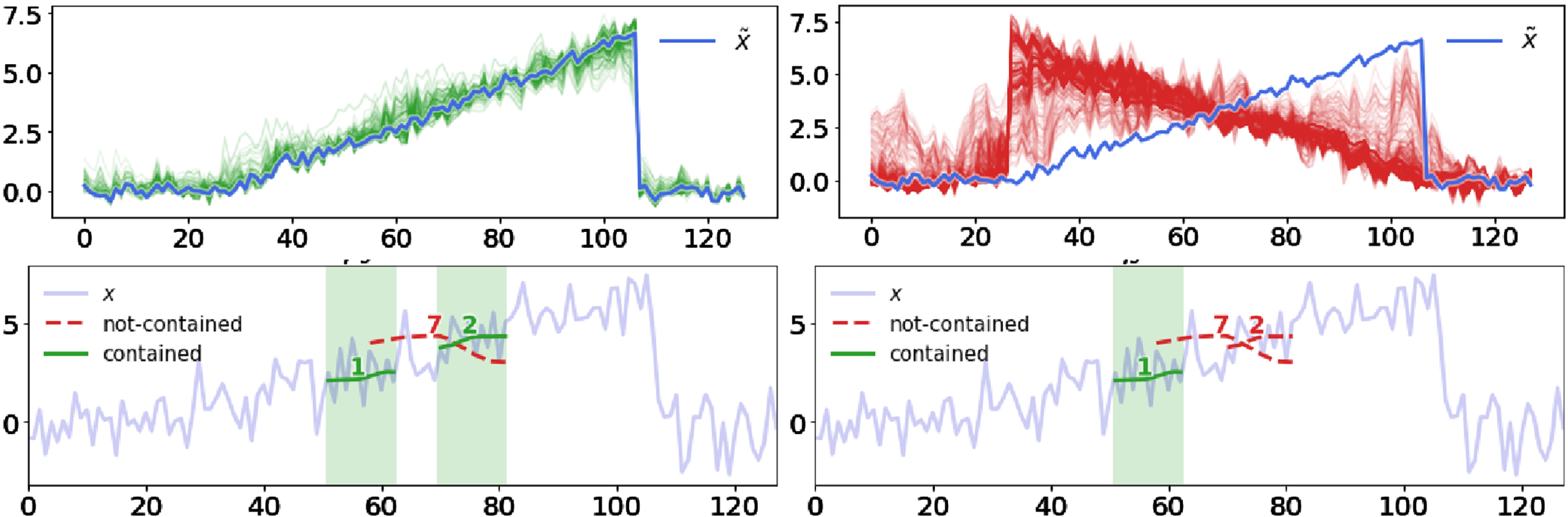
As a running example let consider a time series with length m = 128 belonging to the cylinder-bell-funnel [53] dataset and labeled as bell by a black-box b. lasts represent x with latent space of k = 2, and returns as explanation the content of Figure 4. Figure 4-(top) shows the exemplars (in green) and counter-exemplars (in red). Exemplars have a slope very similar to x and with very low noise. Counter-exemplars can have either a completely different slope with low noise or a slope similar to the one of a bell with very high noise. The exemplars and counter-exemplars are a powerful instance-based part of the explanation that allows users to understand when a time series morphs from one class to another one. The shapelet-based factual and counter-factual rules in Figure 4 (bottom) illustrate the position of the shapelets that must be contained and which are those that must not be contained (at their best alignment with x). The matrix Ξ for our running example is reported in Figure 5 (bottom). Each column represents a time series in $\tilde{H}$ . For each row, a colored cell indicates the presence of the corresponding shapelet, while a white cell indicates the shapelet absence. With respect to the shapelets in Figure 5 (top), exemplars contain shapelets 0, 1, 2, 3, 5, 8, funnel counter-exemplars are similar but without 0, 5 and with 6, 7; cylinder counter-exemplars only contains shapelets 0, 3, 5, 8.

Fig. 4

The time series x under analysis is highlighted in blue in the four plots. From left to tight we have exemplars ${\tilde{H}}_{=}$ , counter-exemplars ${\tilde{H}}_{\neq}$ , shapelet-based factual rule r_s, and counterfactual rules Psi_s. Shapelets are shown at their best alignment.

Fig. 5

Top: Set of shapelets. Bottom: Shapelet matrix. Each column is a time series. For each row, if the shapelet is not contained, the cell is white; it is green if it is an exemplar, red if it is a counter-exemplar.

4.3 Explaining text classifiers

In [35] we design xspells (eXplaining Sentiment Prediction generating ExempLars in the Latent Space), an instantiation of llore to explain text classifiers. Given b, a short text x, e.g., a post on a social network, and the sentiment label y = b (x) assigned by b, e.g., hate or neutral, the explanation provided by xspells is composed of exemplar and counter-exemplar texts, and by the set of most common words in them.

Exemplars are texts close in sentiment to x, and they offer an understanding of what makes the black-box determine the sentiment of texts in the neighborhood of x. Exemplars help in understanding reasons for the sentiment assigned to x. Counter-exemplars help in understanding reasons that would reverse the sentiment assigned. The most common words in the exemplars and counter-exemplars may highlight terms (not necessarily appearing in x) that discriminate between the assigned sentiment and a different sentiment. For xspells we adopted a VAE [33] as AE. Also, differently from abele and lasts that adopt the genetic neighborhood generation, xspells adopts a random neighborhood generation by relying on the fact that the encoder of the VAE maps the data distribution uniformly over the latent space. In addition, xspells guarantees a minimum number of distinct instances by removing duplicates. The explanations returned by xspells are of the form $e = 〈 \tilde{H}, W 〉$ , where $\tilde{H}$ is the set of exemplars and counter-exemplars respecting the latent factual rule r and counterfactual rules Φ (and therefore highly discriminative but similar to each other), and W = W₌ ∪ W_≠ is the set of the h most frequent words in exemplars ${\tilde{H}}_{=}$ and of the h most frequent words in counter-exemplars ${\tilde{H}}_{\neq}$ .

We provide an idea of the explanation returned by xspells for the tweet x =“I dont have any problems with zak, but you seem like a faggot” from the hate dataset [15] labeled as hate by a sentiment classifier b. xspells explanation is:

${\tilde{H}}_{=} = {“ i hate dumb {bitches}^{″}, \dots}$

${\tilde{H}}_{\neq} = {“ this is why i {work}^{″}, “ i really want a {girl}^{″}, \dots}$

W₌ = {(hate, . 22) , (bitches, . 17) , (fat, . 11) , (dumb, . 06) , (wear, . 06)}

W_≠ = {(work, . 06)) , (love, . 06) , (wearing, . 06) , (fuzzy, . 06) , …}

Looking at the exemplars returned by xspells , it is clear that the negative sentiment emerges from the presence of the word “hate”, from sexually degrading references, and derogatory adjectives. On the other hand, counter-exemplars refer to words like “women” and “work” with a positive perspective.

5 Experiments

We experimented with the proposed approaches on various datasets of different types 4 . Three image datasets 5 : the mnist dataset of handwritten digit grayscale images, the fashion dataset is a collection of Zalando’s article grayscale images (e.g. shirt, shoes, bag, etc.), and the cifar10 dataset of colored images of airplanes, cars, birds, cats, etc. Each dataset has ten different labels. Four time series datasets: cylinder-bell-funnel [53] (cbf), epileptic seizure recognition [3] (esr) composed of EEG records with classes indicating the presence/absence of an epileptic seizure, human activity recognition [4] (har) containing signals recorded from a smartphone while performing six different activities, phalanges outlines correct [7] (poc) contains time series representing edges of hand bones images. Two text datasets of tweets: the hate speech dataset [15] (hate) and the polarity dataset (polarity) [47] that contains tweets about movie reviews. Details about the datasets are available in Table 1. For textual data m is the average number of words in a tweet.

Table 1
Datasets statistics and black-box classifiers accuracy

type dataset n m l RF/RES DNN

IMG mnist 70k 28 × 28 10 . 969 . 992

fashion 70k 28 × 28 10 . 865 . 920

cifar10 70k 32 × 32 10 . 460 . 921

TS cbf 0.6k 128 3 1.00 1.00

esr 4.6k 178 2 .978 .972

har 10.3k 561 6 .952 .891

poc 2.6k 80 2 .829 .768

TS hate 5.6k 20.82 2 .925 .848

polarity 10.6k 24.87 2 .670 .630

type	dataset	n	m	l	RF/RES	DNN
IMG	mnist	70k	28 × 28	10	. 969	. 992
	fashion	70k	28 × 28	10	. 865	. 920
	cifar10	70k	32 × 32	10	. 460	. 921
TS	cbf	0.6k	128	3	1.00	1.00
	esr	4.6k	178	2	.978	.972
	har	10.3k	561	6	.952	.891
	poc	2.6k	80	2	.829	.768
TS	hate	5.6k	20.82	2	.925	.848
	polarity	10.6k	24.87	2	.670	.630

We trained and explained away the following black-box classifiers. Random Forest [12] (RF) and Deep Neural Networks (DNN) as implemented by the scikit-learn and keras Python libraries 6 . For mnist and fashion we used a three-layer CNN, while for cifar10 we used the ResNet20 v1 network described in [30]. For time series, besides the CNN and in replacement for the RF, we trained and explained a ResNet (RES) [30] implemented in keras [17]. For text, for the RF, we transformed texts into their TF-IDF weight vectors [58], after removing stop-words, including Twitter stop-words such as “rt”, hashtags, URLs and usernames. Additional details for the various black-box classifiers can be found in [26 , 35].

For every dataset, we used 75% of the available data for training the black-box classifiers. The remaining 25% of data is used for testing the black-box decisions. More specifically, 75% of that testing data is used for training the auto-encoders, and 25% for explaining black-box decisions (explanation set). Classification performance are reported in Table 1.

We compared abele , lasts and xspells against state-of-the-art explainers. We compared most of the methods against lime [51]. We compared abele against the saliency-based explainers in DeepExplain: Saliency (sal) [56], GradInput (grad) [55], IntGrad (intg) [57], ɛ-lrp (elrp) [6], and Occlusion (occ) [63]. We also compared abele against selected by mmd and k-medoids [32] that exploits the maximum mean discrepancy and a kernel function for selecting the best prototypes and criticisms. We compared lasts against shap [40] as detailed in [5]: shapp every time point in the time series becomes a feature, and shaps an a-priori segmentation with predefined length is performed on the time series and a linear interpolation (similar to image explanation) is used as base value by shap .

Details about the parameters of the various explainers and about the AEs ara available in [26 , 35].

5.1 Fidelity evaluation

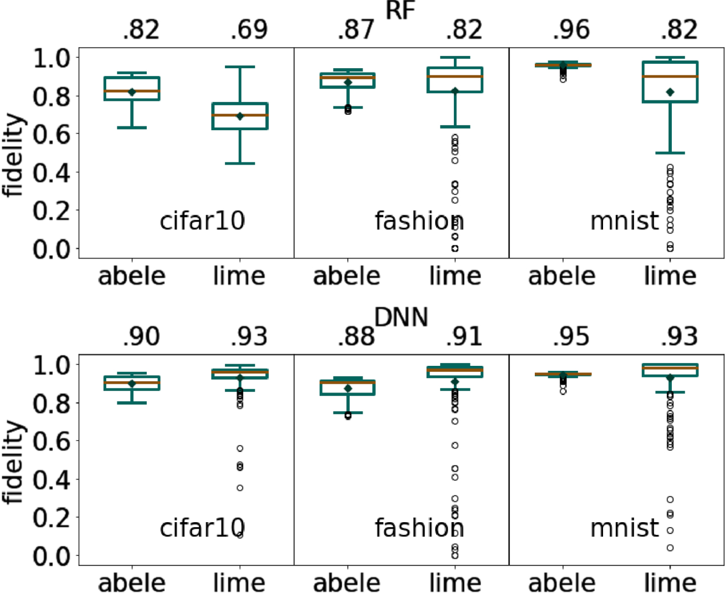
We compared abele , lasts , and xspells against lime in terms of fidelity [16, 25], a metrics suitable for local model-agnostic methods using an interpretable classifier. Fidelity is the ability of an interpretable local model 7 c of mimicking the behavior of a black-box b in the local neighborhood H: $fidelity (H, \tilde{H}) = accuracy (b (\tilde{H}), c (H))$ We report the fidelity of abele in Figure 6. The results show that on all datasets, abele outperforms lime with respect to the RF black-box classifier. For the DNN, the local interpretable classifier of lime is slightly more faithful. However, for both RF and DNN, abele has a fidelity variance markedly lower than lime , i.e., more compact box plots without outliers.

Fig. 6

abele fidelity, numbers on top are the mean values.

We compared lasts against rlasts that, similarly to lime , uses a random neighborhood generation. In addition, we show that extracting an explanation from a local neighborhood is a winning strategy compared to an approach that builds a single global interpretable classifier. Thus, we compared lasts with a shapled-based global decision tree (sbgdt) trained on the partition used by lasts for training the AE. Table 2 reports the values of the fidelity. We observe that lasts outperforms both rlasts and sbgdt . Indeed, the genetic approach allows exploring the neighborhood better than a random approach, while the global approach fails for datasets like har and poc in discovering the local discriminative boundaries.

Table 2

lasts fidelity. Highest values are underlined

dataset	black-box	lasts	rlasts	sbgdt
cbf	RES	1.00	1.00	1.00
	CNN	.889	.917	1.00
esr	RES	1.00	.500	.960
	CNN	1.00	.500	.960
har	RES	.980	.460	.420
	CNN	.860	.440	.400
poc	RES	.500	.400	.660
	CNN	.960	.400	.660

Finally, Table 3 reports the average fidelity of xspells and lime . On the hate dataset, xspells reaches almost perfect fidelity for both black-boxes. lime performances are markedly lower for the RF black-box. On the polarity dataset, the difference is less marked but still in favor of xspells .

Table 3

xspells fidelity. means and standard deviations

	RF		DNN
dataset	lime	xspells	lime	xspells
hate	.62 ±.30	.98 ±.01	.92 ±.15	.98 ±.01
polarity	.89 ±.14	.98 ±.01	.91 ±.20	.97 ±.01

For all the experiments, the non-parametric Friedman test compares the average ranks of explanation methods over multiple datasets and black-boxes w.r.t. the fidelity. The null hypothesis that all methods are equivalent is rejected (p - value < 0.01).

5.2 Usefulness evaluation

The goal of llore -based approaches is to provide exemplars and counter-exemplars as explanations from which a user can easily distinguish the discriminatory traits. Since we could not validate them with an experiment involving humans, inspired by [32], we tested their effectiveness by adopting memory-based machine learning techniques such as the k-nearest neighbor classifier [9] (k-NN). This kind of experiment provides an objective and indirect evaluation of the quality of exemplars and counter-exemplars. In the following experiment we generated n exemplars and counter-exemplars with abele , lasts , and xspells . We compared the discriminatory power of such synthetic instances by selecting from the training set n instances with the same and different labels from x. For comparing against lasts and xspells we selected such instances randomly (named real or baseline in the following), while for comparing against abele we adopted mmd [32] and k-medoids [9]. Then, we used a 1-NN model to classify unseen instances using either the exemplars and counter-exemplars, or using the instances not selected through llore explainers. The classification accuracy of the 1-NN model indicates the exemplars and counter-exemplars usefulness.

In Figure 7 we observe the results for abele . We notice that the usefulness is comparable among the various methods 8 . In particular, when the number of exemplars is low (1 ≤ n ≤ 4), abele outperforms mmd and k-medoids . This effect reveals that, on the one hand, just a few exemplars and counter-exemplars generated by abele are good for recognizing the real label, but if the number increases, then the 1-NN is getting confused. On the other hand, mmd is more effective when n is higher as it selects a discriminative set of images for the 1-NN classifier.

Fig. 7

abele usefulness through 1-NN accuracy varying the number of (counter-)exemplars.

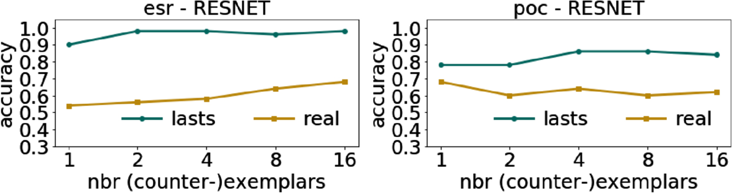
Figure 8 shows the average accuracy of lasts and real that randomly selects real instances. We notice that lasts clearly overcomes real. Indeed, exemplars and counter-exemplars help discover the decision boundary and highlight similarities and differences. The performance of lasts are on average high and constant in every dataset, also revealing that few exemplars and counter-exemplars are a good proxy for recognizing the classification outcome. On the other hand, the accuracy of real only increases for esr with increasing n. This result shows that not every time series is suitable for recognizing a class, but they are as such only if carefully selected like lasts does.

Fig. 8

lasts usefulness as 1-NN accuracy.

Finally, Figure 9 shows the usefulness for xspells that neatly overcomes the baseline. The difference is particularly marked when n is small. Even though the difference tends to decrease for large n’s, large-sized explanations are less useful in practice due to the cognitive limitations of human evaluators. Moreover, xspells performances are quite stable w.r.t. n, i.e., even one or two exemplars and counter-exemplars are sufficient to let the 1-NN classifier distinguish the sentiment assigned to x in an accurate way.

Fig. 9

xspells usefuless as 1-NN accuracy.

5.3 Stability evaluation

Explainers stability is a fundamental property to gain the user’s trust and to guarantee a reliable service [29]. We asses the stability of lasts in terms of coherence: similar instances labeled with the same class should get similar explanations. Inspired by the local Lipschitz estimation [2] we design the incoherence of an explanation e for an instance x as: ${incoherence}_{N_{x}} (x) = \frac{∥ e_{x^{(f)}} - e_{x} ∥^{2}}{∥ e_{x^{(c)}} - e_{x} ∥^{2}}$ where $N_{x} = {x_{i} \in X_{e} | dist (x_{i}, x) \leq ɛ}$ is the neighborhood of x defined in terms of a distance function dist, x^(c) and x^(f) are respectively the closest and furthest instance to x in $N_{x}$ in terms of dist, e_x, e_{x
^(c)}, e_{x
^(f)} are their explanations, and ∥e_a - e_b ∥ ² is a similarity function between explanations e_a and e_b. We refer the reader to specific papers for definitions of the similarity functions. Thus, the lower is the incoherence, the more stable is the explanation. Values lower than one indicates that the similarity between the explanations of similar instances is higher than the similarity between dissimilar instances. We highlight that, in the rest of this work, we report this value both as incoherence and as coherence. In this case, the reasoning on the scores is the opposite.

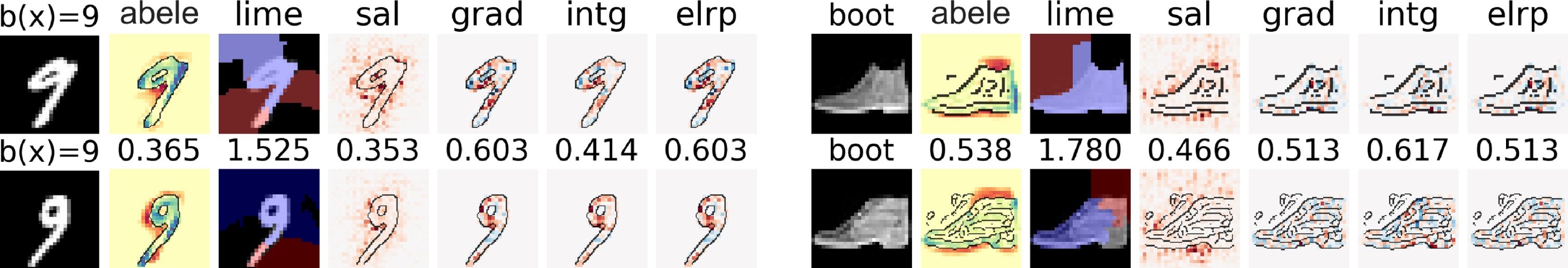
Table 4 reports mean and standard deviation of the incoherence for abele and its competitors. As showed in [2], our results confirm that lime does not provide robust explanations, grad and intg are the best performers, and abele performance is comparable to them in terms of coherence. This high resilience of abele is due to the usage of AAE, which is also adopted for image denoising [59]. Figure 10 compare the saliency maps of a selected image from mnist and fashion labeled with DNN. Numbers on the top represent the ratio in the robustness formula. Although there is no change in the black-box outcome, we can observe how for some of the other explainers like lime , elrp , and grad , the saliency maps vary considerably. On the other hand, abele ’s explanations remain coherent and stable. We can observe how in both nines and boots the fundamental yellow area does not change, especially within the image’s edges. In addition, also the red and blue parts, which can be varied without impacting on the classification, are almost identical, e.g. the boots’ neck and the sole in Figure 10.

Table 4
abele incoherence for DNN. The lower the better

dataset abele elrp grad intg lime occ sal

cifar10 . 575 ± .10 . 542 ± .08 . 542 ± .08 . 532 ± .11 1.919 ± .25 1.08 ± .23 . 471 ± .05

fashion . 451 ± .06 . 492 ± .10 . 492 ± .10 . 561 ± .17 1.618 ± .16 . 904 ± .23 . 413 ± .03

mnist . 380 ± .03 . 740 ± .21 . 740 ± .21 . 789 ± .22 1.475 ± .14 . 734 ± .21 . 391 ± .03

dataset	abele	elrp	grad	intg	lime	occ	sal
cifar10	. 575 ± .10	. 542 ± .08	. 542 ± .08	. 532 ± .11	1.919 ± .25	1.08 ± .23	. 471 ± .05
fashion	. 451 ± .06	. 492 ± .10	. 492 ± .10	. 561 ± .17	1.618 ± .16	. 904 ± .23	. 413 ± .03
mnist	. 380 ± .03	. 740 ± .21	. 740 ± .21	. 789 ± .22	1.475 ± .14	. 734 ± .21	. 391 ± .03

Fig. 10

Saliency maps for mnist and fashion comparing images with the same DNN outcome; numbers on the top is the incoherence.

Table 5 reports the median incoherence for lasts . Results show that lasts returns explanations much more coherent than those returned by shap and with values markedly lower. The non-parametric Friedman test for the incoherence rejected the null hypothesis that all methods are equivalent (p - value < 0.0001). Figure 11 reports the box plots showing all the incoherence values for the har dataset. We notice that incoherence of lasts explanations can vary a lot, while the incoherence of shap explanations is stably around one. This fact is not necessarily a weakness because it indicates that also among similar time series lasts finds a variegate array of similar explanations but with different causes.

Table 5

lasts median incoherence. Lowest values are underlined

	RES			CNN
dataset	lasts	shapp	shaps	lasts	shapp	shaps
cbf	.16	.99	.94	.52	.99	.94
esr	1.0	.99	.92	.81	.99	.98
har	.68	.99	.99	.77	1.0	1.0
poc	.90	.99	.98	.85	.99	.97

Fig. 11

LASTS incoherence for har and poc.

Finally, Table 6 reports the average coherence over the explanation set. xspells and lime have comparable levels of coherence and an even number of cases where one overcomes the other. A Welch’s t-test shows that the difference of the coherence indexes between xspells and lime is statistically significant (p-value <0.01) in only one case, namely for the polarity dataset and RF black-box model.

Table 6

xspells mean and stdev of the coherence. The closer to 1 the

dataset	RF		DNN
lime	xspells	lime	xspells
hate	1.10 ± 0.17	1.05 ± 0.25	1.06 ± 0.08	1.12 ± 0.39
polarity	1.05 ± 0.15	1.15 ± 0.20	1.13 ± 0.18	1.09 ± 0.14

6 Conclusion

We have presented llore , a local model-agnostic and data-agnostic explanation framework using the latent feature space learned through an autoencoder for the synthetic neighborhood generation process. The explanation returned by llore consists of exemplar and counter-exemplar instances, labeled respectively with the class identical to, and different from, the class of the instance to explain. We instantiated llore fore images, time series and text realizing abele , lasts , and xspells , respectively. Each of them augments the explanation of llore with a data-specific logic-based explanation. An extensive experimental comparison with state-of-the-art explainers shows that llore -based approaches address their deficiencies and outperforms them by returning meaningful, stable, useful, and understandable explanations.

The method has some limitations. First, the pre-training of an autoencoder is mandatory. This requires the availability of a certain amount of data and the study necessary to realize the autoencoder effectively. We highlight that this point is crucial because, as shown in [43], a not negligible effort is necessary to train the autoencoder that enables llore to work depending on the problem faced and on the data type. Second, the explainer performance strictly depends on the autoencoder adopted: a better autoencoder would lead to more realistic exemplars and counter-exemplars. A future goal would be to determine the minimum amount of data required to have reliable explanations. In particular, xspells does not return very satisfactory results in terms of plausibility of the neighborhood generated. We plan to refine its neighborhood generation exploiting the approaches presented in [36, 39]. Third, llore is a local explanation approach with its ensuing limitations. Also, each llore instantiation has further specific limitations. We refer the interested reader to the individual papers for further details on data-specific future extensions and limitations. Fourth, even though the various implementations have shown promising results for different datasets and black-box models, it is still impossible to justify for which dataset, task, and black-box model an explainer should be preferred to another one. Indeed, so far, we can only say that llore -based approaches are better than their competitors in the settings experimented. As future work, we would like to generalize these assumptions to derive guidelines suggesting the best implementation for every setting. Finally, as already done in [43], it would be essential to assess with a human evaluation the effectiveness of the explanations returned by llore -based approaches.

Footnotes

Acknowledgments

This work has been partially supported by the European Community Horizon 2020 programme under the funding schemes: H2020-INFRAIA-2019-1: Research Infrastructure G.A. 871042 SoBigData++, G.A. 952026 HumanE-AI Net, ERC-2018-ADG G.A. 834756 XAI: Science and technology for the eXplanation of AI decision making, G.A. 952215 TAILOR, CHIST-ERA grant CHIST-ERA-19-XAI-010, by MUR (N. not yet available), FWF (N. I 5205), EPSRC (N. EP/V055712/1), NCN (N. 2020/02/Y/ST6/00064), ETAg (N. SLTAT21096), BNSF (N. KP-06-AOO2/5). A special thank goes to the co-authors of the original works, i.e., Anna Monreale, Francesco Spinnato, Orestis Lampridis, Salvatore Ruggieri, Stan Matwin, Dino Pederschi and Fosca Giannotti.

The EU General Data Protection Regulation establishes a “right to explanation” for any automated decision acting on individuals.

More details can be found in [].

https://github.com/riccotti/ABELE, https://github.com/fspinna/TS_AgnosticLocalExplainer, .

http://yann.lecun.com/exdb/mnist/, https://www.kaggle.com/zalando-research/fashionmnist .

https://scikit-learn.org/stable/, .

Decision tree for llore methods, linear regressor for lime.

Similar results for RF not reported due to lack of space.

References

Adadi

and Berrada

, Peeking inside the black-box: A survey on explainable artificial intelligence (XAI), IEEE Access 6 (2018), 52138–52160.

Alvarez-Melis

and Jaakkola

T.S.

, Towards robust interpretability with self-explaining neural networks. In NeurIPS (2018), pp. 7786–7795.

Andrzejak

, Lehnertz

, Mormann

, Rieke

, David

and Elger

, Indications of nonlinear deterministic and finitedimensional structures in time series of brain electrical activity, Physical Review E 64 (2002), 061907, 01 2002.

Anguita

, Ghio

, Oneto

, Parra

and Reyes-Ortiz

J.L.

, A public domain dataset for human activity recognition using smartphones. In ESANN, 2013.

Arnout

, El-Assady

, Oelke

and Keim

D.A.

, Towards A rigorous evaluation of XAI methods on time series. In ICCV Workshops, (2019), pp. 4197–4201, IEEE.

Bach

, Binder

, et al., On pixel-wise explanations for nonlinear classifier decisions by layer-wise relevance propagation, PloS One 10(7) (2015), e0130140.

Bagnall

A.J.

and Davis

L.M.

, Predictive modelling of bone age through classification and regression of bone shapes, CoRR, 1406.4781, 2014.

Berk

, Heidari

, Jabbari

, Kearns

and Roth

, Fairness in criminal justice risk assessments: The state of the art, Sociological Methods & Research 50(1) (2018), 3–44.

Bien

and Tibshirani

, Prototype selection for interpretable classification, The Annals of Applied Statistics (2011), pp. 2403–2424.

10.

Bodria

, Giannotti

, Guidotti

, Naretto

, Pedreschi

and Rinzivillo

, Benchmarking and survey of explanation methods for black box models. CoRR, 2102.13076, 2021.

11.

Bowman

S.R.

, Vilnis

, Vinyals

, Dai

A.M.

, Jozefowicz

and Bengio

, Generating sentences from a continuous space. In CoNLL, pp. 10–21. ACL, 2016.

12.

Breiman

, Random forests, Mach Learn 45(1) (2001), 5–32.

13.

Byrne

R.M.J.

, Counterfactuals in explainable artificial intelligence (XAI): evidence from human reasoning. In IJCAI, pp. 6276–6282, ijcai.org, 2019.

14.

Chen

, Li

, Tao

, Barnett

, Rudin

and Su

, This looks like that: Deep learning for interpretable image recognition. In NeurIPS (2019), pp. 8928–8939.

15.

Davidson

, Warmsley

, Macy

M.W.

and Weber

, Automated hate speech detection and the problem of offensive language. In ICWSM, pp. 512–515. AAAI Press, 2017.

16.

Doshi-Velez

and Kim

, Towards a rigorous science of interpretable machine learning. arXiv:1702.08608, 2017.

17.

Fawaz

H.I.

, Forestier

, Weber

, et al., Data augmentation using synthetic data for time series classification with deep residual networks. CoRR, 1808.02455, 2018.

18.

Freitas

A.A.

, Comprehensible classification models: a position paper, SIGKDD Explor 15(1) (2013), 1–10.

19.

Frixione

and Lieto

, Prototypes vs exemplars in concept representation. In KEOD, pp. 226–232. SciTePress, 2012.

20.

Goebel

, Chander

, Holzinger

, Lecue

, Akata

, Stumpf

, Kieseberg

and Holzinger

, Explainable AI: the new 42? In CD-MAKE, volume 11015 of Lecture Notes in Computer Science, (2018), pp. 295–303. Springer, 2018.

21.

Goodfellow

I.J.

, Pouget-Abadie

, Mirza

, Xu

, Warde-Farley

, Ozair

, Courville

A.C.

and Bengio

, Generative adversarial nets. In NIPS (2014), pp. 2672–2680.

22.

Grabocka

, Schilling

, Wistuba

and Schmidt-Thieme

, Learning time-series shapelets. In KDD, (2014), pp. 392–401. ACM.

23.

Guidotti

and Monreale

, Designing shapelets for interpretable data-agnostic classification. In AIES, (2021), pp. 532–542. ACM.

24.

Guidotti

, Monreale

and Cariaggi

, Investigating neighborhood generation methods for explanations of obscure image classifiers. In PAKDD (1), volume 11439 of Lecture Notes in Computer Science, pp. 55–68. Springer, 2019.

25.

Guidotti

, Monreale

, Giannotti

, Pedreschi

, Ruggieri

and Turini

, Factual and counterfactual explanations for black box decision making, IEEE Intell Syst 34(6) (2019), 14–23.

26.

Guidotti

, Monreale

, Matwin

and Pedreschi

, Black box explanation by learning image exemplars in the latent feature space. In ECML/PKDD (1), volume 11906 of Lecture Notes in Computer Science, pp. 189–205. Springer, 2019.

27.

Guidotti

, Monreale

, Ruggieri

, Turini

, Giannotti

and Pedreschi

, A survey of methods for explaining black box models, ACM Comput Surv 51(5) (2019), 93:1–93:42.

28.

Guidotti

, Monreale

, Spinnato

, Pedreschi

and Giannotti

, Explaining any time series classifier. In CogMI, (2020), pp. 167–176. IEEE.

29.

Guidotti

and Ruggieri

, On the stability of interpretable models. In IJCNN, pp. 1–8. IEEE, 2019.

30.

, Zhang

, Ren

and Sun

, Deep residual learning for image recognition. In CVPR, pp. 770–778. IEEE Computer Society, 2016.

31.

Hinton

G.E.

and Salakhutdinov

R.R.

, Reducing the dimensionality of data with neural networks, Science 313(5786) (2006), 504–507.

32.

Kim

, Koyejo

and Khanna

, Examples are not enough, learn to criticize! criticism for interpretability. In NIPS (2016), pp. 2280–2288.

33.

Kingma

D.P.

and Welling

, Auto-encoding variational bayes. In ICLR, 2014.

34.

Lakkaraju

, Bach

S.H.

and Leskovec

, Interpretable decision sets: A joint framework for description and prediction. In KDD, (2016), pp. 1675–1684, ACM.

35.

Lampridis

, Guidotti

and Ruggieri

, Explaining sentiment classification with synthetic exemplars and counterexemplars. In DS, volume 12323 of Lecture Notes in Computer Science, pp. 357–373. Springer, 2020.

36.

Lei

, Barzilay

and Jaakkola

T.S.

, Rationalizing neural predictions. In EMNLP, pp. 107–117. The Association for Computational Linguistics, 2016.

37.

X.-H.

, Cao

C.C.

, Shi

, et al., A survey of data-driven and knowledge-aware explainable AI. TKDE, 2020.

38.

Lines

, Davis

L.M.

, Hills

and Bagnall

A.J.

, A shapelet transform for time series classification. In KDD, pp. 289–297. ACM, 2012.

39.

Liu

, Yin

and Wang

W.Y.

, Towards explainable NLP: A generative explanation framework for text classification. In ACL (1), pp. 5570–5581. Association for Computational Linguistics, 2019.

40.

Lundberg

S.M.

and Lee

, A unified approach to interpreting model predictions. In NIPS (2017), pp. 4765–4774.

41.

Makhzani

, Shlens

, Jaitly

and Goodfellow

I.J.

, Adversarial autoencoders. CoRR, 1511.05644, 2015.

42.

Malgieri

and Comande

, Why a right to legibility of automated decision-making exists in the GDPR, IDPL 7(4) (2017), 243–265.

43.

Metta

, Guidotti

, Yin

, Gallinari

and Rinzivillo

, Exemplars and counterexemplars explanations for image classifiers, targeting skin lesion labeling. In ISCC, pp. 1–7. IEEE, 2021.

44.

Miller

, Explanation in artificial intelligence: Insights from the social sciences, Artif Intell 267 (2019), 1–38.

45.

Molnar

, Interpretable machine learning. Lulu. com, 2019.

46.

Ntoutsi

, et al., Bias in data-driven Artificial Intelligence systems - An introductory survey, DAMI 10(3), 2020.

47.

Pang

and Lee

, Seeing stars: Exploiting class relationships for sentiment categorization with respect to rating scales. In Proc. of the Annual Meeting of the Association for Computational Linguistics (ACL), (2005), pp. 115—124.

48.

Pasquale

, The black box society: The secret algorithms that control money and information, Harvard University Press, 2015.

49.

Pedreschi

, Giannotti

, Guidotti

, Monreale

, Ruggieri

and Turini

, Meaningful explanations of black box AI decision systems. In AAAI, pp. 9780–9784, AAAI Press, 2019.

50.

Plumb

, Molitor

and Talwalkar

A.S.

, Model agnostic supervised local explanations. In NeurIPS (2018), pp. 2520–2529.

51.

Ribeiro

M.T.

, Singh

and Guestrin

, “why should I trust you?”: Explaining the predictions of any classifier. In KDD, pp. 1135–1144, ACM, 2016.

52.

Rudin

, Stop explaining black box machine learning models for high stakes decisions and use interpretable models instead, NMI, pp. 206, 05 2019.

53.

Saito

, Local feature extraction and its applications using a library of bases, PhD thesis, Yale University, 1994.

54.

Schlegel

, Lam

D.V.

, Keim

D.A.

and Seebacher

, Tsmule: Local interpretable model-agnostic explanations for time series forecast models. CoRR, 2109.08438, 2021.

55.

Shrikumar

, Greenside

, Shcherbina

and Kundaje

, Not just a black box: Learning important features through propagating activation differences, CoRR, 1605.01713, 2016.

56.

Simonyan

, Vedaldi

and Zisserman

, Deep inside convolutional networks: Visualising image classification models and saliency maps. In ICLR (Workshop Poster), 2014.

57.

Sundararajan

, Taly

and Yan

, Axiomatic attribution for deep networks. In ICML, volume 70 of Proceedings of Machine Learning Research, pp. 3319–3328, PMLR, 2017.

58.

Tan

P.-N.

, Steinbach

and Kumar

, Introduction to Data Mining, Pearson Education India, 2016.

59.

Xie

, Xu

and Chen

, Image denoising and inpainting with deep neural networks. In NIPS (2012), pp. 350–358.

60.

Yang

, Rudin

and Seltzer

M.I.

, Scalable bayesian rule lists. In ICML, volume 70 of Proceedings of Machine Learning Research, pp. 3921–3930, PMLR, 2017.

61.

and Keogh

E.J.

, Time series shapelets: a new primitive for data mining. In KDD, pp. 947–956. ACM, 2009.

62.

and Keogh

E.J.

, Time series shapelets: a novel technique that allows accurate, interpretable and fast classification, Data Min Knowl Discov 22(1-2) (2011), 149–182.

63.

Zeiler

M.D.

and Fergus

, Visualizing and understanding convolutional networks. In ECCV (1), volume 8689 of Lecture Notes in Computer Science, pp. 818–833. Springer, 2014.