Towards a unified model for symbolic knowledge extraction with hypercube-based methods

Abstract

The XAI community is currently studying and developing symbolic knowledge-extraction (SKE) algorithms as a means to produce human-intelligible explanations for black-box machine learning predictors, so as to achieve believability in human-machine interaction. However, many extraction procedures exist in the literature, and choosing the most adequate one is increasingly cumbersome, as novel methods keep on emerging. Challenges arise from the fact that SKE algorithms are commonly defined based on theoretical assumptions that typically hinder practical applicability.

This paper focuses on hypercube-based SKE methods, a quite general class of extraction techniques mostly devoted to regression-specific tasks. We first show that hypercube-based methods are flexible enough to support classification problems as well, then we propose a general model for them, and discuss how they support SKE on datasets, predictors, or learning tasks of any sort. Empirical examples are reported as well –based upon the PSyKE framework –, showing the applicability of hypercube-based methods to actual classification tasks.

Keywords

Explainable AI knowledge extraction interpretable prediction PSyKE

1 Introduction

One of the main features to be underpinned by a believable human-agent interaction is explainability. Along this line, symbolic knowledge extraction (SKE) is a powerful tool within the scope of explainable artificial intelligence (XAI). It enables reverse-engineering of the black-box (BB) machine learning algorithms—nowadays exploited in many artificial intelligence tasks [25]. SKE allows data scientists to associate human-comprehensible, post-hoc explanations [18] to the recommendations or decisions computed by the most common prediction-effective –yet, poorly interpretable –algorithms. For instance, SKE is widely adopted for credit-risk evaluation [3, 38], medical diagnosis [5, 13], credit card screening [36], intrusion detection systems [15], keyword extraction [2], and space mission data prediction [33].

The basic idea behind SKE is to construct symbolic (hence interpretable) models mimicking the behaviour of the pre-existing BB predictors to be explained. Symbolic models should describe BB in terms of the outputs they provide as responses to (classes of) input values. Symbols, in particular, may consist of intelligible knowledge—e.g., lists or trees of logic rules that can be exploited to obtain predictions as well as to better understand the underlying predictor. In other words, symbols are in principle both human- and machine-interpretable.

Because of the many SKE techniques available in the literature, selecting the most appropriate SKE algorithm for a given learning task may become cumbersome. Difficulties may derive from the intrinsic design choices behind each extraction algorithm. In fact, SKE algorithms may commonly target specific learning tasks (classification or regression), specific sorts of machine learning (ML) predictors (e.g. neural networks, support vector machines, linear models, etc.), or specific sorts of training data (e.g. continuous, categorical, or binary).

We focus upon a quite general class of SKE techniques, which we denote as hypercube-based methods, that extract symbolic knowledge by querying black-box predictors as oracles, and by recursively partitioning the input spaces of these BB into several hypercubes. Even though commonly considered regression-specific, we show that hypercube-based SKE methods are flexible enough to deal also with classification problems. More generally, we propose a common model for hypercube-based methods, and we show how they can be exploited to perform SKE on data sets, predictors, or learning tasks of any sort.

Accordingly, the contribution of this paper is manifold. First, we provide a general and abstract description of any hypercube-based SKE workflow. Second, we discuss how hypercube-based methods can be engineered to provide full support to supervised learning tasks—there including regression and classification ones. Third, we compare existing hypercube-based procedures (e.g. ITER [16], GridREx [31]) w.r.t. the methods used to partition the input space, approximate black-box decisions, and construct the extracted symbolic knowledge. Finally, to demonstrate the versatility of hypercube-based methods, we analyse disparate SKE scenarios via the PSyKE framework [8 , 32]—that is, a platform combining SKE and Semantic Web to provide human-interpretability and intelligent agent-interoperability for BB-based machine learning tasks.

2 State of the art

2.1 Knowledge extraction

Computational systems are considered interpretable when humans are able to easily understand their operation and outcomes [10]. However, nowadays decision support systems often rely on ML models having excellent predictive capabilities at the expense of interpretability. These sub-symbolic predictors of growing complexity, which learn input-output relations from data and store them as internal parameters, do not provide any kind of symbolic representation of the acquired knowledge, thus lacking an interpretable representation to the benefit of human users. ML algorithms are defined as black boxes for this reason [20].

It is possible to preserve the impressive BB predictive performance and, at the same time, obtain human-intelligible clues or explanations regarding the BB behaviour by substituting the opaque model with a mimicking interpretable surrogate. The XAI community, indeed, has proposed a number of means to produce ex-post explanations for sub-symbolic predictors in the form of surrogate models based on sets of rules extracted from the underlying opaque model. Amongst the proposals there are methods to extract lists [11 , 31] or trees [6, 12] of logic rules, usually if-then-else, M-of-N or fuzzy. SKE is particularly important also for another reason: it may enable further manipulations—for instance, to merge the know-how of different BB models [9].

Knowledge extraction algorithms can be categorised along three orthogonal dimensions [7]: (i) supported learning tasks, (ii) shape of the symbolic knowledge provided in output, (iii) approach for dealing with the underlying ML models, usually known as translucency.

Supported tasks –item (i) –are usually supervised classification or regression. A cluster of SKE algorithms can only explain BB classifiers –e.g. Rule-extraction-as-learning [11], TREPAN [12] and others [4, 21] –, while a different cluster is designed to support BB regressors—e.g., ITER [16], GridEx [31], GridREx [27] and others [34 , 37]. Finally, a little subset of SKE techniques is able to handle both tasks, as for the case of G-Rex [19] and CART [6].

As far as the shape of the output knowledge is concerned –item (ii) –, decision rules [14 , 22] and trees [23, 24] are usually considered the most human-understandable ways to represent knowledge. This is why most SKE methods produce one of these two structures as output. Regardless of the shape, conditions describing decision rules and nodes are expressed by using the same input/output data types adopted to train the underlying BB. For instance, SKE procedures applied to classifiers accepting N-dimensional numerical data and providing K distinct output classes will produce rule lists or trees involving a certain number of predicates over N input variables x₁, …, x_n and having K possible outcomes. A further categorisation may be performed w.r.t. the kind of predicates contained in the output knowledge. In particular, it is possible to observe conjunctions or disjunctions of inequalities (e.g. x_i ≷ c) as well as inclusions in or exclusions from intervals (e.g. x_i ∈ [l, u]) for numerical data. Categorical data are usually associated to equalities (e.g. x_i = c) and set-inclusions (e.g. x_i ∈ {c₁, c₂, …}). M-of-N or fuzzy rules are other available alternatives.

Finally, the translucency dimension –item (iii) –represents the strategy adopted by the SKE algorithm to obtain interpretable knowledge from a BB. In particular, extractors may be decompositional or pedagogical [1, 7]. Decompositional techniques consider the internal structure of the underlying BB, hence producing symbolic knowledge which mimics how it internally works. As a side-effect, decompositional algorithms are bound to specific sorts of ML predictors—and possibly introduce constraints on their internal structures. For instance, techniques tailored to neural networks are not applicable to support vector machines. Similarly, procedures explicitly designed for 3-layered networks are not suitable for deeper ones. On the other hand, pedagogical methods can extract symbolic knowledge without relying on any information about the inner structure of predictors. They simply query the predictor as an oracle, observing its response to particular inputs, and generalise its behaviour accordingly. For this reason, pedagogical extractors come with no constraints on the sorts of predictors they can be applied to. Hence, they are more general –despite potentially being less precise –but considerations about the output performance strictly depend on the task at hand.

To evaluate the quality of SKE techniques different indicators are exploited, depending on the task to solve. Common choices are readability, fidelity and predictive performance measurements [26, 39], but also other ad hoc metrics have been recently proposed [28]. The former expresses how interpretable is the output knowledge from the human perspective. It is generally evaluated through the number of extracted rules and the number of constraints per rule. Fidelity is related to the capability of the extracted knowledge to mimic the underlying BB predictions, whereas predictive performance measurements are assessed by comparing the predictions drawn from the extracted knowledge with the ground truth. Measurements involving predictions should be assessed via the same scoring function used for the underlying BB—which in turn strictly depends on the performed task. Classifiers are usually evaluated via accuracy, precision, recall, and F₁ score. Conversely, common metrics for regressors are the mean absolute/squared error (MAE/MSE) and the R score.

2.2 Existing knowledge-extraction methods

In the following an overview of the hypercube-based SKE algorithms cited in Section 4 – namely ITER and GridEx –is provided. Differences in the input space partitioning and in the decision approximation are highlighted in particular. Output rules are lists of logic rules in both cases. It is worth noting that both algorithms assume input features to be continuous and may be applied to any kind of BB predictor, being pedagogical SKE methods.

2.2.1 ITER

The ITER algorithm [16] is based on the iterative creation and expansion of hypercubes inside the input feature space until a maximum number of iterations is reached, or, the whole input space is covered. Expansion may stop also if it is not possible to further expand the hypercubes. In those cases, additional cubes may be created to cover the remaining space.

ITER is limited to regression tasks by design and performs averaging operations to associate output values to hypercubes. For each cube, ITER selects all the training samples inside and calculates the mean prediction by using the underlying BB as an oracle. If the training samples are not enough to satisfy the minimum amount specified by the user, extra random samples are generated and predicted along with the others.

ITER also takes advantage of a similarity criterion to expand hypercubes. In particular, at every iteration, all the possible expansions around each cube are considered, but only one is performed, i.e., the one capable of expanding a cube towards the most similar input space region. The similarity is calculated via the mean absolute difference between the output values of the cubes to be expanded and the eligible cubes around them.

2.2.1 GridEx

The GridEx algorithm [31] can be considered as an extension of ITER aimed at overcoming its major drawback, i.e., the non-exhaustivity of its output rules. GridEx achieves this goal because it is exhaustive by design. Unlike ITER , GridEx adopts a top-down approach to split the input feature space into hypercubes. It iteratively partitions the whole space according to some defined strategies, marking at each iteration if the created partitions are negligible (i.e., they contain no training samples, so they are discarded since it is not relevant to have rules associated to them), eligible for further partitioning (if they contain samples that are not enough similar), or permanent (otherwise, if they contain similar training instances and, thus, these cubes should have good predictive performance). Strategies to split the input space are fixed if the user specifies for each iteration how many partitions have to be performed along all the input dimensions, or adaptive if the number of splits is determined through the relevance of each input feature w.r.t. the output variable. Since GridEx has been designed exclusively for regression tasks, as ITER , also in this case output decisions are obtained via local averaging calculations, and actual regression rules are not supported.

The similarity between samples is assessed through the output value standard deviation of all the instances included inside a hypercube. If the standard deviation is below a user-defined threshold, then the cube only contains similar samples and it is not further partitioned. Otherwise, GridEx attempts to split the cube into smaller regions, possibly enclosing more similar samples. Since the readability of the output model depends on the number of extracted rules, it is of paramount importance to keep it as low as possible. For this reason, a merging phase is performed after every splitting iteration as an optimisation to reduce the number of rules. Indeed, adjacent cubes are pairwise merged according to a similarity criterion on the contained samples. The merging phase is iterative: at each step are merged only the two adjacent cubes that result in the merged hypercube having the lowest standard deviation, and it terminates when it is not possible to further merge cubes without exceeding the standard deviation user-defined threshold.

A first GridEx generalisation supporting regression rules as output decisions led to the GridREx algorithm [27]. GridREx can extract fully regressive rules, with a linear combination of the input variables as a postcondition. Even though all the other details are identical to GridEx , GridREx achieves better predictive performance, fidelity, and readability than GridEx .

2.3 PSyKE

The PSyKE [8 , 32] software library is a Python framework providing general-purpose support to SKE. It can be exploited to obtain logic rules from BB classifiers and regressors via several pedagogical extraction methods. Its unified API allows users to select the most adequate procedure with few lines of code, also allowing fast comparison between different alternatives. At the time of writing, PSyKE supports 6 state-of-the-art SKE algorithms (see Table 1 for further details), allowing researchers and data scientists to exploit them without the need to implement and test them.

Table 1
Knowledge-extraction algorithms supported by PSyKE : summary

Algorithm Ref. Task Input Features Output type Knowledge Shape

REAL [11] Classification Binary String label Rule list

TREPAN [12] Classification Binary String label Decision tree

ITER [16] Regression Continuous Numerical constant Rule list

GridEx [31] Regression Continuous Numerical constant Rule list

GridREx [27] Regression Continuous Regression law Rule list

CART [6] Classification, Regression Any String label, Numerical constant Decision tree

Algorithm	Ref.	Task	Input Features	Output type	Knowledge Shape
REAL	[11]	Classification	Binary	String label	Rule list
TREPAN	[12]	Classification	Binary	String label	Decision tree
ITER	[16]	Regression	Continuous	Numerical constant	Rule list
GridEx	[31]	Regression	Continuous	Numerical constant	Rule list
GridREx	[27]	Regression	Continuous	Regression law	Rule list
CART	[6]	Classification, Regression	Any	String label, Numerical constant	Decision tree

The PSyKE design is developed around the notion of extractor, intended as any algorithm accepting as input an ML predictor (classifier or regressor) together with the data set used to train it, and providing as output a theory of logic rules extracted from the predictor. PSyKE extractors need additional information about the data set to give more human-interpretability to the extracted knowledge. In particular, a schema of the data set can be given as input to formally describe input and output feature names and types.

PSyKE also exhibits utilities to manipulate the data set and perform feature engineering, for instance, procedures to discretise or scale continuous features and to one-hot encode discrete/discretised features. In addition, there are automatic procedures to select the optimal parameters for extractors, which manual tuning may be challenging for human users.

As for the knowledge provided in output by extractors, it is possible to choose between two options: (i) a Prolog theory composed of human-intelligible clauses, possibly simplified to ease readability; (ii) an OWL ontology having agent-interpretable SWRL rules, to pursue interoperability between intelligent agents [32]. Input data as well may follow Semantic Web encoding, so PSyKE extractors accept tabular data or knowledge graphs stored in OWL ontologies.

3 Hypercube-based knowledge extractors

The general model for hypercube-based extractors presented here is aimed at extending their application to classification tasks other than regression tasks. Hypercube-based extraction methods are pedagogical extraction procedures that can operate on trained ML predictors of any sort. They consider the predictor P undergoing extraction as an oracle to be queried multiple times, in order to find a partitioning H₁ ∪ … ∪ H_n of its input space $X$ such that the output space $Y$ can be expressed for each partition. Hence, they extract knowledge in the form of rule lists or trees, where each rule attempts to describe the outcome of P for a particular hypercube $H_{i} \subseteq X$ . Rules have the following logical form: $x \in H_{i} \to (y = f_{i} (x))$ to be read as “if the input vector $x \in X$ is in some hypercube H_i, then the prediction $y \in Y$ is f_i (x)”, where f_i (x) is a function approximating P outcomes. Note that each hypercube H_i is a partition of the input space $X$ , and f_i is the function approximating P outcomes related to that hypercube (could be a constant, a linear function, etc.), i.e.: f_i (x) ≈ P (x) , ∀ x ∈ H_i.

Hypercube-based extraction procedures should then attempt to select hypercubes and local approximation functions so as to maximise the fidelity of the overall rule set/list w.r.t. P. Accordingly, they follow a pretty linear workflow, which may be roughly summarised in 3 steps, namely:

partitioning the input space into disjoint hypercubes H₁, …, H_n, following a selected strategy and according to possible defined constraints;

approximating the prediction of P for each hypercube H_i, via some function f_i; and

creating a rule set where each rule concisely represents the behaviour of P in H_i via f_i.

In the following, we delve into the details of all the aforementioned phases.

3.1 Input space partitioning

Input space partitioning is a recursive computation aimed at finding the optimal number, shape, and size of hypercubes w.r.t. some desiderata, such as: (i) covering the whole input space; (ii) obtaining disjoint regions; (iii) minimising the number of regions; (iv) maximising the similarity amongst the samples inside single regions; (v) minimising the predictive error correlated to each partition.

These conditions cannot be all satisfied simultaneously, especially when dealing with high-dimensional data sets. Thus, some requirements may be relaxed. For instance, the input space coverage may be limited only to interesting hypercubes, neglecting the others. Let us consider a hypercube ‘interesting’ if it contains training samples, as it may have a role to play in drawing future predictions.

Alternatively, the partitioning process may terminate after a predefined number of iterations, as some state-of-the-art algorithms actually do. However, this may lead to the indiscriminate exclusion of some regions of the input space that are not negligible. In turn, the explained model will not be able to provide predictions for a subset of input instances.

Non-contiguous hypercubes may be relaxed into hierarchical or fuzzy regions, possibly mapped into non-overlapping rules, in order to have unambiguous output predictions.

3.2 Similarity and fidelity

The amount of hypercubes an input space is partitioned into may significantly impact the interpretability of the final symbolic model. In fact, hypercube-based methods will output as many rules as the hypercubes they have partitioned the input space into—and of course more (or more complex) rules imply lower readability for the human user.

The capability of grouping together similar samples into a single hypercube is so quintessential for supporting the creation of few, general, and simple rules which capture the behaviour of the original predictor with high fidelity. This corresponds to (i) data points from the same hypercube drawing similar predictions, and to (ii) predictions having a high fidelity (or, equivalently, low error rates) w.r.t. to the original predictor. Accordingly, here we delve into the details of how to assess (i) similarity amongst data points from contiguous hypercubes, as well as (ii) predictive errors between a candidate rule and the underlying predictor.

3.2.1 Similarity amongst instances

Input space partitions can be considered similar according to the following definitions:

input closeness if input variables of both subregions have values ranging in similar domains, as for adjacent disjoint or overlapping regions;

output closeness if the output associated with the instances in the two subregions is similar.

While it is straightforward to check input closeness (e.g., through Euclidean distance), dealing with output closeness requires taking into account the learning problem at hand.

As far as classification is concerned, we may consider two hypercubes H₁ and H₂ as output-close w.r.t. a predictor P if (and only if) the most frequent output class is the same in both hypercubes: $H_{1} \overset{P}{\approx} H_{2} \Leftrightarrow mode (P (H_{1})) = mode (P (H_{2}))$ (1) where mode (·) denotes the statistical operator returning the most frequent item over a set, and P (H) is a shortcut standing for {P (x) : x ∈ H}, to lighten the notation.

Conversely, in the case of regression with constant outputs, output-similarity may be expressed as a function of the absolute difference between the mean output predictions performed by the predictor P on the two hypercubes H₁ and H₂: $H_{1} \overset{P}{\approx} H_{2} \Leftrightarrow | mean (P (H_{1})) - mean (P (H_{2})) | < θ$ (2) where θ is a parameter defining the strictness of the similarity criterion.

Equation 2 does not capture the similarity amongst hypercubes characterised by high variability of P. In such a case a more complex solution is required: $\begin{matrix} H_{1} \overset{P}{\approx} H_{2} \Leftrightarrow \frac{mae (f_{1, 2}, H_{1} \cup H_{2})}{mae (f_{1}, H_{1}) + mae (f_{2}, H_{2})} \leq \frac{1}{2} \end{matrix}$ (3) where mae (f, H) is the mean absolute error of the linear function f in approximating P for data in H. In other words, H₁ and H₂ are output-similar if it is possible to (i) merge the two hypercubes, (ii) find a linear combination f_1,2 of the input variables representing the input/output relationship of the so merged regions, and (iii) reach a predictive performance of f_1,2 better than the average performance of the linear functions f₁, f₂ associated with the corresponding separated subregions.

For instance, Figure 1 reports examples of similarity assessments calculated for a theoretical generalised hypercube-based extractor applied to a classification task (Figure 1a) and to a regression task (Figures 1b and c). Figures concerning the regression task represent constant and non-constant extractor outputs, respectively. The example assumes a 2-dimensional data set with continuous input features both ranging in the interval [0, 5]. In the figures, hypercubes to be expanded/merged are those having coloured backgrounds. Possible adjacent hypercubes to be joined to them are represented as hypercubes having no background. Adjacent hypercubes that are similar to the hypercubes to be expanded are represented with a hatched background. It is worth noting that for the example depicted in Fig. 1b a similarity threshold θ equal to 5.0 has been chosen. In Fig. 1c the predictive errors corresponding to the adjacent hypercubes as well as the calculated errors of the possible merged regions are omitted for the clarity of the image.

Fig. 1

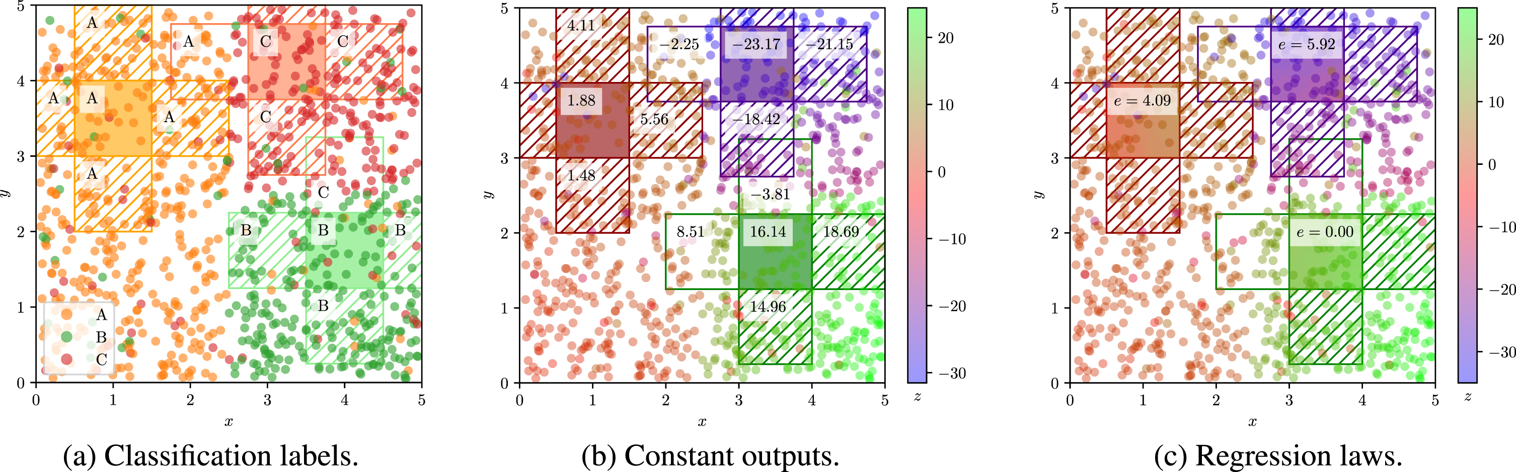
Two-dimensional example of different similarities calculated for generalised extractors. Hatched regions are suitable to be merged with the adjacent one (coloured background). In 1c the predictive error e is reported inside the three central hypercubes.

3.2.2 Predictive error assessment

A generalised metric is necessary to evaluate the predictive performance of a set of rules for both classifications and regressions. We propose the following function as an error function for a rule set R applied to a data set D: $error (R, D) = {\begin{matrix} mae (R, D) & (regression) \\ 1 - accuracy (R, D) & (classification) \end{matrix}$ (4) where mae (R, D) and accuracy (R, D) are the mean absolute error and the classification accuracy score, respectively, calculated on the output predictions obtained via the rules in R, for the data set D, and w.r.t. the expected outputs for D.

Figure 2 reports some examples of predictive errors measured for a generalised extractor by assuming a 2-dimensional data set with continuous input features both ranging in the [0, 5] interval. The figure represents a classification task and two regression tasks. The first regression task is approximated by the extractor with constant outputs, whereas the second is associated with non-constant outputs. The predictive error e is reported as misclassifications in the first case and absolute error in the others.

Fig. 2

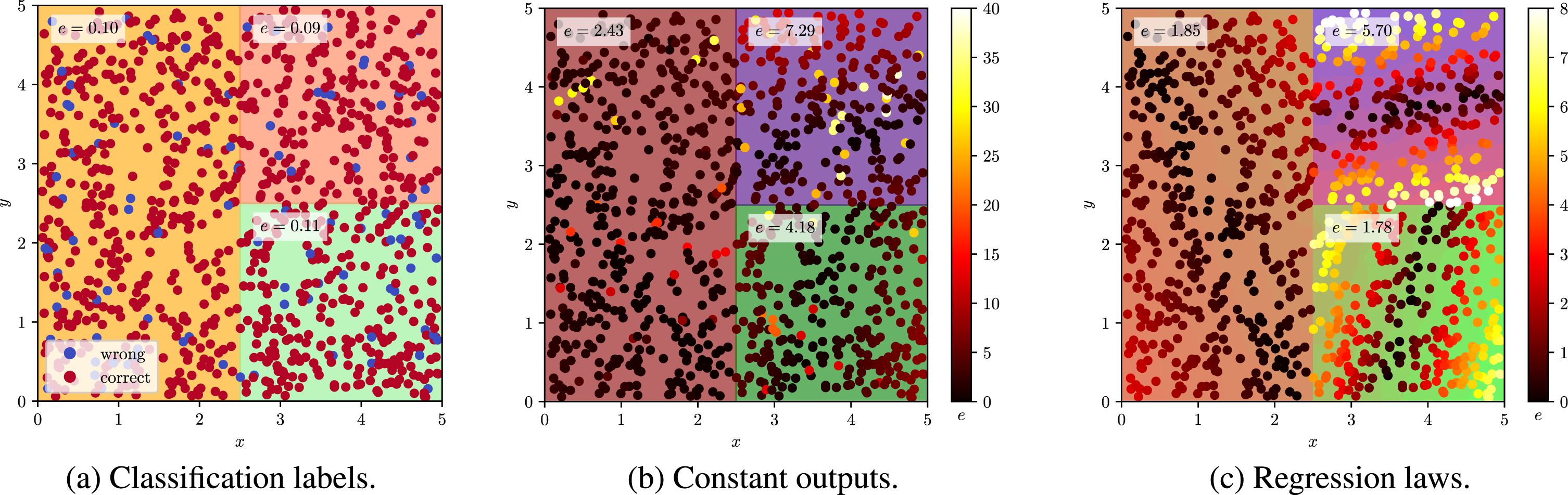
Two-dimensional example of different predictive errors measured for generalised extractors. The predictive error e is reported for each region.

3.3 Approximating predictions

As for the approximation of output predictions associated with each hypercube, approximated outputs are usually computed on the basis of the predictions provided by the underlying BB when applied to an extended training set. The extended training set may consist of the original data the predictor has been trained upon –or a subset of it –possibly augmented with some further data. Data augmentation via random input samples is useful to attain higher predictive performance, provided that the predictor is used as an oracle to compute the corresponding expected outputs.

Provided that the input space has been adequately partitioned into several hypercubes, the prediction associated with each hypercube may consist of (i) a constant numerical value (e.g., ITER , GridEx) or, (ii) a linear combination of the input variables (e.g., GridREx). The latter option, in particular, is well-suited for regression tasks, while the former may support both classification and regression tasks.

To choose the best output value for each hypercube, one may either (i) aggregate the predictions corresponding to all available points in that hypercube –e.g. via the ‘mean’, ‘mode’, or ‘median’ statistical aggregation functions –, or (ii) fit a local function locally approximating the predictor in that hypercube. Again, which option is better really depends on the learning task the underlying predictor has been designed for.

Figure 3 reports examples of predictions provided by a generalised extractor—assuming a 2-dimensional data set with continuous input features both ranging in the [0, 5] interval, as in previous examples. The figure shows a classification task and two regression tasks, where the former regression task is approximated by the extractor with constant outputs. Background colour represents the output provided by the extractor.

Fig. 3

Two-dimensional example of different predictions provided by generalised extractors.

3.4 Output rule set creation

After selecting a set of input space regions and one output decision for each of them, hypercube-based extractors build a rule set, each rule composed of a precondition and a postcondition. The precondition is a formal description of a single input region in terms of individual features, for instance by means of value inclusion inside an interval. Hypercubic n-dimensional regions may be described through the conjunction of (at most) n interval inclusion conditions. On the other hand, the postcondition is simply the decision calculated for the region on the basis of the task at hand, as previously described. Thus, extracted human-readable logic rules generally have the following format: $\begin{matrix} Output is O if X_{1} \in [l_{1}, u_{1}], X_{2} \in [l_{2}, u_{2}], . . ., X_{n} \in [l_{n}, u_{n}] \end{matrix}$ where O is the output decision and X₁, X₂, . . . , X_n are input variables with values in the intervals described by corresponding lower- and upper-bounds l_i and u_i.

4 Experiments: PSyKE

We exemplify the effectiveness of hypercube-based methods by considering the implementations of the ITER and GridEx extraction algorithms. Both methods are designed for regression and here applied to classification tasks. CART is used as a benchmark to assess the predictive performance of the modified extractors, since it is a state-of-the-art procedure directly applicable to data sets described by continuous features, without prior discretisation. All the adopted implementations are included in the PSyKE framework. 1

Experiments are executed on the well-known Iris data set, 2 composed of 150 instances corresponding to Iris flower individuals. Each instance is described by 4 continuous input features (i.e., petal and sepal width and length of the exemplary) and a categorical class label (i.e., the species of the exemplary). Three different species are present in the Iris data set (namely, Setosa, Virginica, and Versicolor) and they are equally balanced (50 individuals per species).

The experiments are carried out as follows: (i) the data set is randomly split into training and test sets, of equal size; (ii) a k-nearest neighbour (k-NN) classifier is trained on the training set; (iii) three different extractors are used to extract symbolic rules out of that classifier; (iv) the predictive performance of both the classifier and the extracted rules are graphically compared –in terms of decision boundaries –, and numerically assessed—in terms of accuracy and F₁ scores. In the case of the extracted rules, fidelity and readability measurements are performed as well. It is worth noting that the training set is used only to train the models. Conversely, the test set is used only to assess the predictive performance of the predictor and extractors. Both sets are constant for each experiment, to better compare the performance under the same conditions. The fidelity of the extracted rules (w.r.t. the predictor they have been extracted from) is assessed as well, via the same metrics adopted for the predictive performance. Finally, the output knowledge readability is expressed as the number of extracted rules.

4.1 Predictor training

Extraction techniques require an underlying BB to be used as an oracle. This is why we trained and compared several k-NN classifiers, with different values for the k hyper-parameter. Table 2 predictor reports details on the accuracy and F₁ scores measured for each model. The best predictive performance is achieved by the 9-NN. Consequently, in the following, all the discussed extractors are applied to it. The decision boundaries of the selected 9-NN are reported in Fig. 4a.

Table 2
Accuracy and F₁ scores for several k-NN predictors

Accuracy F₁ score

k score Setosa Virginica Versicolor

3 0.93 1.00 0.89 0.92

5 0.96 1.00 0.94 0.95

7 0.96 1.00 0.94 0.95

9 0.97 1.00 0.96 0.97

11 0.95 1.00 0.91 0.94

13 0.93 1.00 0.89 0.92

15 0.93 1.00 0.89 0.92

17 0.96 1.00 0.94 0.95

	Accuracy	F₁ score
3	0.93	1.00	0.89	0.92
5	0.96	1.00	0.94	0.95
7	0.96	1.00	0.94	0.95
9	0.97	1.00	0.96	0.97
11	0.95	1.00	0.91	0.94
13	0.93	1.00	0.89	0.92
15	0.93	1.00	0.89	0.92
17	0.96	1.00	0.94	0.95

Fig. 4

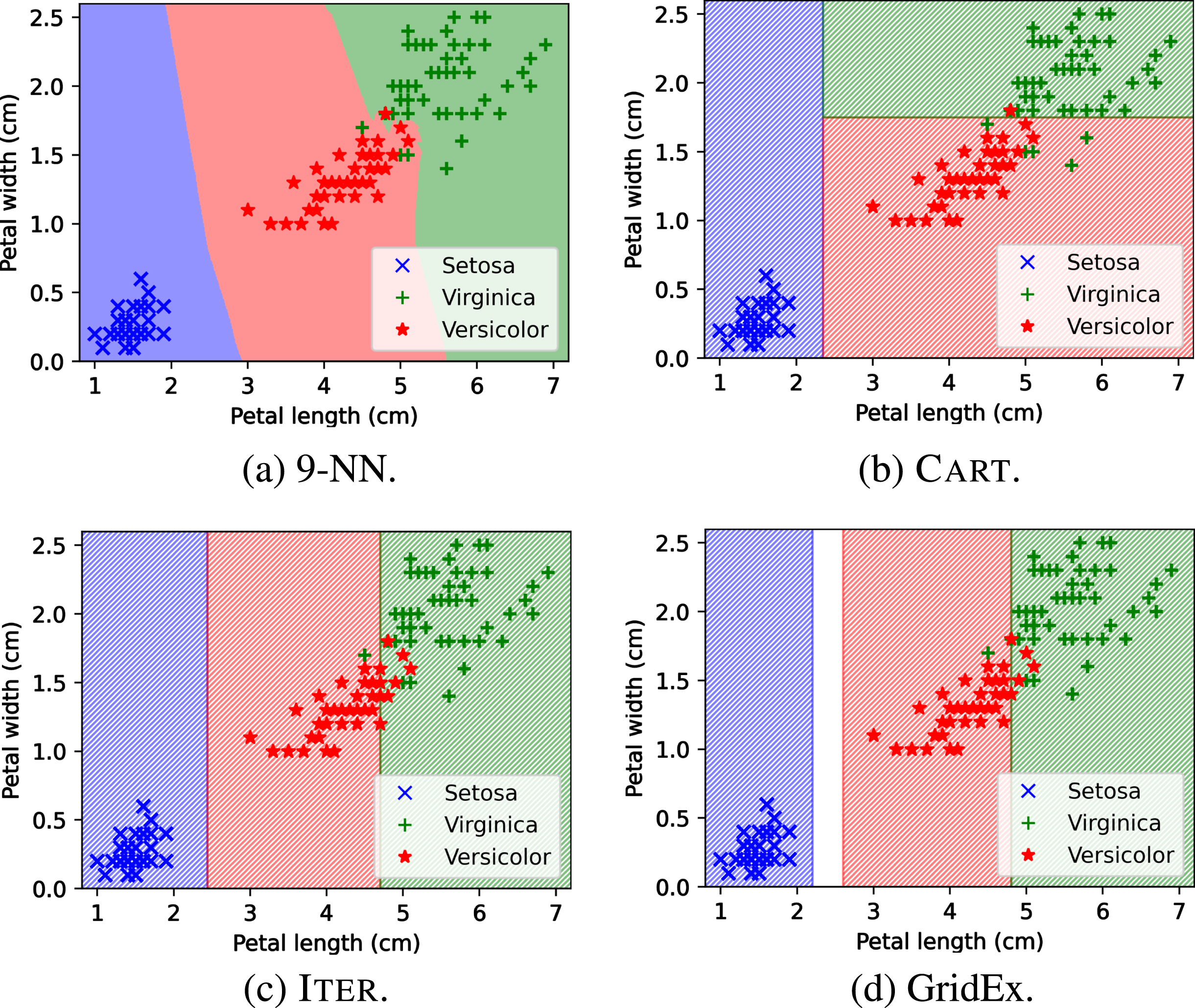
Decision boundaries corresponding to the 9-NN predictions and to the rules extracted with 3 different extractors for the Iris data set. Only the two most relevant features are reported.

4.2 CART

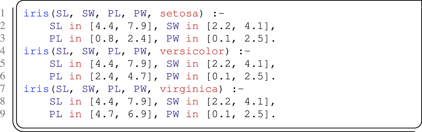
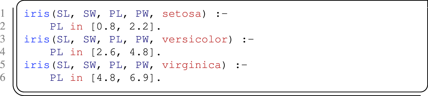
The CART extractor is applied to the 9-NN classifier to extract human-intelligible knowledge in Prolog syntax, without discretising the input data set. Unlike ITER and GridEx , CART is able to work upon discretised data sets too. Training the model with a maximum leaf amount of 3 gives the following theory, composed of 3 rules—namely, one per each possible class of the Iris data set.

The theory is always exhaustive since it is always possible to find a leaf classifying an instance. Table 3 reports numerical assessments of the predictive performance and fidelity of the theory extracted with CART . Fig. 4b reports the input space partitioning induced by the theory. Here, only petal width and length are considered to assign class labels to input instances.

Table 3
Accuracy and F₁ scores observed for CART applied to the 9-NN classifier. Fidelity measurements are reported inside the parentheses

Accuracy F₁ score

# of rules score Setosa Virginica Versicolor

3 0.95 (0.95) 1.00 (1.00) 0.91 (0.91) 0.94 (0.94)

	Accuracy	F₁ score
3	0.95 (0.95)	1.00 (1.00)	0.91 (0.91)	0.94 (0.94)

The computational complexity of CART –intended as the required time to extract the knowledge from a BB –is dependent on the corresponding tree dimension and, therefore, it is directly proportional to the maximum amount of leaves and/or to the maximum allowed depth. The same holds for the complexity of the input space partitioning.

4.3 ITER

The ITER algorithm has been applied as well to explain the 9-NN classifier. We test several hyper-parameter values in order to attain the rule list having the highest possible predictive performance and fidelity. ITER is based on the following hyper-parameters: (i) the size for updating cubes, s, expressed as a fraction of input dimension (i.e., 0.1 means a tenth of the interval between minimum and maximum values of each dimension); (ii) the number of starting points, n, representing the initial hypercubes; (iii) the minimum number of examples to consider in each cube; (iv) the similarity threshold between adjacent cubes, θ, that is not relevant for classification; (v) the maximum number of iterations, fixed to 600.

The results of our experiments for ITER are reported in Table 4. The best predictive performance, achieved with the parameters highlighted in bold font in the table, corresponds to the following rules.

Table 4
Comparing accuracy and F₁ scores of several ITER instances

Update Starting Min. # of Accuracy F₁ score

size points examples rules score Setosa Virginica Versicolor

0.10 1 75 4 0.84 (0.87) 1.00 (1.00) 0.81 (0.84) 0.78 (0.82)

0.10 1 150 4 0.84 (0.87) 1.00 (1.00) 0.81 (0.84) 0.78 (0.82)

0.10 3 75 3 0.84 (0.87) 1.00 (1.00) 0.81 (0.84) 0.78 (0.82)

0.10 3 150 4 0.84 (0.87) 1.00 (1.00) 0.81 (0.84) 0.78 (0.82)

0.07 1 75 3 0.94 (0.97) 1.00 (1.00) 0.92 (0.96) 0.93 (0.97)

0.07 1 150 3 0.94 (0.97) 1.00 (1.00) 0.92 (0.96) 0.93 (0.97)

0.07 3 75 4 0.94 (0.97) 1.00 (1.00) 0.92 (0.96) 0.93 (0.97)

0.07 3 150 6 0.94 (0.97) 1.00 (1.00) 0.92 (0.96) 0.93 (0.97)

Update	Starting	Min.	# of	Accuracy	F₁ score
0.10	1	75	4	0.84 (0.87)	1.00 (1.00)	0.81 (0.84)	0.78 (0.82)
0.10	1	150	4	0.84 (0.87)	1.00 (1.00)	0.81 (0.84)	0.78 (0.82)
0.10	3	75	3	0.84 (0.87)	1.00 (1.00)	0.81 (0.84)	0.78 (0.82)
0.10	3	150	4	0.84 (0.87)	1.00 (1.00)	0.81 (0.84)	0.78 (0.82)
0.07	1	75	3	0.94 (0.97)	1.00 (1.00)	0.92 (0.96)	0.93 (0.97)
0.07	1	150	3	0.94 (0.97)	1.00 (1.00)	0.92 (0.96)	0.93 (0.97)
0.07	3	75	4	0.94 (0.97)	1.00 (1.00)	0.92 (0.96)	0.93 (0.97)
0.07	3	150	6	0.94 (0.97)	1.00 (1.00)	0.92 (0.96)	0.93 (0.97)

The input space partitioning induced by the extracted rules is shown in Fig. 4c.

The computational time complexity of ITER applied to a data set having d input features is $O (\frac{n \cdot 2^{d}}{θ s})$ , while the input space partitioning complexity is $O (\frac{n}{θ})$ . Indeed, the required time depends on the amount of input features d, of starting cubes n as well as on the number of new cubes created during the algorithm execution according to the similarity threshold θ and on the size of the unitary cube expansion s. Large values for n and d as well as small values for θ and s imply higher computational time. On the other hand, the amount of output partitions only depends on n and θ.

4.4 GridEx

Finally, as the last step of our experiments, the GridEx extractor is applied to the 9-NN classifier. In this case as well, different values for the hyper-parameters have been explored. We recall that fundamental hyper-parameters for GridEx are (i) the depth of the recursive partitioning, Δ (i.e., how many iterations); (ii) the number of slices to perform at every iteration, n; (iii) the error threshold used to decide if further divide a hypercube, θ, fixed to 0.1 for all experiments; (iv) the minimum number of examples to consider in each cube, here fixed to 1. As for the number of slices to be performed, adaptive strategies are preferred to fixed strategies. Experiment results concerning GridEx are reported in Table 5. The best hyper-parameter values are highlighted in bold font. The semantics of adaptive splitting strategies described by the couple (a, b) is the following: all input dimensions having relevance greater than a are split into b subregions at each iteration. All the other dimensions are not split. Input feature relevance is always scaled in the [0, 1] interval. Corresponding output Prolog theory and input space partitioning are reported in the following and in Fig. 4d, respectively.

Table 5
Comparing accuracy and F₁ scores of GridEx instances with different hyper-parameters

Adaptive Accuracy F₁ score

Depth strategy # of rules score Setosa Virginica Versicolor

1 (0.85, 5) 3 0.87 (0.90) 1.00 (1.00) 0.84 (0.87) 0.82 (0.86)

1 (0.85, 8) 3 0.94 (0.97) 1.00 (1.00) 0.92 (0.96) 0.93 (0.96)

1 (0.85, 10) 3 0.87 (0.90) 1.00 (1.00) 0.84 (0.87) 0.82 (0.86)

2 (0.85, 5) 6 0.89 (0.91) 1.00 (1.00) 0.86 (0.88) 0.83 (0.88)

2 (0.85, 8) 6 0.94 (0.97) 1.00 (1.00) 0.92 (0.96) 0.93 (0.96)

2 (0.85, 10) 6 0.89 (0.91) 1.00 (1.00) 0.86 (0.88) 0.83 (0.88)

2 (0.75, 5) 8 0.93 (0.94) 1.00 (1.00) 0.89 (0.91) 0.91 (0.93)

2 (0.75, 2) 11 0.69 (0.69) 0.87 (0.87) 0.74 (0.74) 0.39 (0.39)

	Adaptive		Accuracy	F₁ score
1	(0.85, 5)	3	0.87 (0.90)	1.00 (1.00)	0.84 (0.87)	0.82 (0.86)
1	(0.85, 8)	3	0.94 (0.97)	1.00 (1.00)	0.92 (0.96)	0.93 (0.96)
1	(0.85, 10)	3	0.87 (0.90)	1.00 (1.00)	0.84 (0.87)	0.82 (0.86)
2	(0.85, 5)	6	0.89 (0.91)	1.00 (1.00)	0.86 (0.88)	0.83 (0.88)
2	(0.85, 8)	6	0.94 (0.97)	1.00 (1.00)	0.92 (0.96)	0.93 (0.96)
2	(0.85, 10)	6	0.89 (0.91)	1.00 (1.00)	0.86 (0.88)	0.83 (0.88)
2	(0.75, 5)	8	0.93 (0.94)	1.00 (1.00)	0.89 (0.91)	0.91 (0.93)
2	(0.75, 2)	11	0.69 (0.69)	0.87 (0.87)	0.74 (0.74)	0.39 (0.39)

Also in this case only one input feature is considered to draw predictions. The partitioning is exhaustive w.r.t. the data set, however, a small input space region is neglected since the algorithm observed no instances included in it. Differently from ITER , GridEx is able to detect input dimensions that do not affect the classification. In this manner all the non-relevant antecedents are dropped from the output theory, resulting in a higher human-readability.

The computational time complexity of GridEx applied to a data set having d input features is $O (Δ)$ , whereas the input space partitioning complexity is $O (d^{\frac{n Δ}{θ}})$ . Indeed, required time depends on the depth of the partitioning, whereas the amount of output partitions is equal to n for each input feature (= dⁿ), for each one of the Δ iterations (= d^nΔ). During the merging phase the number of partitions is reduced according to the θ threshold, thus larger θ values imply fewer output partitions (and vice versa).

4.5 Discussion

In this subsection we compare the results of CART , ITER , and GridEx applied to the Iris data set, all summarised in Figure 4. Results are compared on the basis of readability, fidelity, and predictive performance, other than the decision boundaries induced by the extracted rules. As for readability, all the extractors are equivalent w.r.t. the number of rules, since they are able to extract one predictive rule per output class. Conversely, the readability of ITER is hindered by the number of antecedents per rule, since it produces a constraint for each input dimension. Under this perspective, CART and GridEx are able to keep amongst the rules’ conditions only those involving relevant features to perform the classification, resulting in a fourth of the total amount of antecedents w.r.t. ITER .

The decision boundaries provided by GridEx and ITER are more similar to those produced by the underlying k-NN, but no sensible difference in the classification accuracy is noticeable, since all extractors present a score between 0.94 and 0.95 (we recall that the 9-NN has an accuracy score equal to 0.97). The same reasoning may be performed about the extractors’ fidelity, equal to 0.95 for CART and 0.97 for ITER and GridEx .

Finally, GridEx does not provide a classification rule for a small input space region, since it finds that region as negligible (no data set instances belong to it).

5 Conclusions

In this paper we generalise the class of hypercube-based knowledge extractors, usually designed for applications in regression tasks, in order to demonstrate their suitability in classification tasks as well. We therefore propose a common model for these methods and a concrete implementation within the PSyKE framework. The generalised model presented here considers how algorithmic patterns currently adopted by hypercube-based SKE extractors can be relaxed to widen their applicability scopes, achieving competitive overall performance w.r.t. ad hoc existing alternatives.

Acknowledgments

This paper has been partially supported by (i) the EU ICT-48 2020 project TAILOR (No. 952215), and (ii) the CHIST-ERA IV project “Expectation” (CHIST-ERA-19XAI-005), co-funded by the EU and the Italian MUR.

Conflict of interests

The authors have no conflict of interest to declare.

Footnotes

Code available at https://github.com/psykei/psyke-python

https://archive.ics.uci.edu/ml/datasets/iris

References

Andrews

, Diederich

and Tickle

A.B.

, Survey and critique of techniques for extracting rules from trained artificial neural networks, Knowledge-Based Systems8(6) (1995), 373–389.

Azcarraga

, Liu

M.D.

and Setiono

, Keyword extraction using backpropagation neural networks and rule extraction, In The 2012 International Joint Conference on Neural Networks (IJCNN 2012), IEEE, 2012, pp. 1–7.

Baesens

, Setiono

, Mues

and Vanthienen

, Using neural network rule extraction and decision tables for credit-risk evaluation, Management Science49(3) (2003), 312–329.

Barakat

and Diederich

, Eclectic rule-extraction from support vector machines, International Journal of Computer and Information Engineering2(5) (2008), 1672–1675.

Bologna

and Pellegrini

, Three medical examples in neural network rule extraction, Physica Medica13 (1997), 183–187.

Breiman

, Friedman

, Stone

C.J.

and Olshen

R.A.

, Classification and Regression Trees. CRC Press, 1984.

Calegari

, Ciatto

and Omicini

, On the integration of symbolic and sub-symbolic techniques for XAI: A survey, Intelligenza Artificiale14(1) (2020), 7–32.

Calegari

and Federico

, The PSyKE technology for trustworthy artificial intelligence, 13796, 2023, pp. 3–16. XXI International Conference of the Italian Association for Artificial Intelligence, AIxIA 2022, Udine, Italy, 2022, Proceedings.

Ciatto

, Calegari

, Omicini

and Calvaresi

, Towards XMAS: Explainability through Multi-Agent Systems. In AI&IoT 2019 – Artificial Intelligence and Internet of Things 2019, volume 2502 of CEUR Workshop Proceedings, 2019, pp. 40–53.

10.

Ciatto

, Calvaresi

, Schumacher

M.I.

and Omicini

, An abstract framework for agent-based explanations in AI, In 19th International Conference on Autonomous Agents and Multi Agent Systems, IFAAMAS, 2020, pp. 1816–1818.

11.

Craven

M.W.

and Shavlik

J.W.

, Using sampling and queries to extract rules from trained neural networks, In Machine Learning Proceedings 1994, Elsevier, 1994, pp. 37–45.

12.

Craven

M.W.

and Shavlik

J.W.

, Extracting treestructured representations of trained networks, In Advances in Neural Information Processing Systems 8. Proceedings of the 1995 Conference, The MIT Press, 1996, pp. 24–30.

13.

Franco

, Subirats

J.L.

, Molina

, Alba

and Jerez

J.M.

, Early breast cancer prognosis prediction and rule extraction using a new constructive neural network algorithm, In Computational and Ambient Intelligence, volume 4507 of LNCS, Springer, 2007, pp. 1004–1011.

14.

Freitas

A.A.

, Comprehensible classification models: A position paper, ACM SIGKDD Explorations Newsletter15(1) (2014), 1–10.

15.

Hofmann

, Schmitz

and Sick

, Rule extraction from neural networks for intrusion detection in computer networks, In 2003 IEEE International Conference on Systems, Man and Cybernetics, volume 2, IEEE, 2003, pp. 1259–1265.

16.

Huysmans

, Baesens

and Vanthienen

, ITER: An algorithm for predictive regression rule extraction, In Data Warehousing and Knowledge Discovery (DaWaK 2006), Springer, 2006, pp. 270–279.

17.

Huysmans

, Dejaeger

, Mues

, Vanthienen

and Baesens

, An empirical evaluation of the comprehensibility of decision table, tree and rule based predictive models, Decision Support Systems51(1) (2011), 141–154.

18.

Kenny

E.M.

, Ford

, Quinn

and Keane

M.T.

, Explaining black-box classifiers using post-hoc explanations-by-example: The effect of explanations and error-rates in XAI user studies, Artificial Intelligence294 (2021), 103459.

19.

Konig

, Johansson

and Niklasson

, G-REX: A versatile framework for evolutionary data mining, In 2008 IEEE International Conference on Data Mining Workshops (ICDM 2008 Workshops), 2008, pp. 971–974.

20.

Lipton

Z.C.

, The mythos of model interpretability, Queue16(3) (2018), 31–57.

21.

Martens

, Baesens

, Gestel

T.V.

and Vanthienen

, Comprehensible credit scoring models using rule extraction from support vector machines, European Journal of Operational Research183(3) (2007), 1466–1476.

22.

Murphy

P.M.

and Pazzani

M.J.

, ID2-of-3: Constructive induction of M-of-N concepts for discriminators in decision trees, In Machine Learning: Proceedings of the Eight International Workshop (ML91), Morgan Kaufmann Publishers, Inc., San Mateo, CA, USA, 1991, pp. 183–187.

23.

Quinlan

J.R.

, Simplifying decision trees, International Journal of Man-Machine Studies27(3) (1987), 221–234.

24.

Quinlan

J.R.

, C4.5: Programming for machine learning. Morgan Kauffmann, 1993.

25.

Rocha

, Papa

J.P.

and Meira

L.A.A.

, How far do we get using machine learning black-boxes?International Journal of Pattern Recognition and Artificial Intelligence26(02) (2012), 1261001–(1–23).

26.

Sabbatini

and Calegari

, Evaluation metrics for symbolic knowledge extracted from machine learning black boxes: A discussion paper, In Workshop on Explainable AI in Finance @ICAIF 2022, New York City, 2022.

27.

Sabbatini

and Calegari

, Symbolic knowledge extraction from opaque machine learning predictors: GridREx & PEDRO, In 19th International Conference on Principles of Knowledge Representation and Reasoning (KR 2022), Haifa, Israel, IJCAI, 2022, pp. 554–563.

28.

Sabbatini

and Calegari

, On the evaluation of the symbolic knowledge extracted from black boxes, In AAAI 2023 Spring Symposium Series (to appear), San Francisco, California, 2023.

29.

Sabbatini

, Ciatto

, Calegari

and Omicini

, On the design of PSyKE: A platform for symbolic knowledge extraction, In WOA 2021 – 22nd Workshop “From Objects to Agents”, volume 2963 of CEUR Workshop Proceedings, 2021, pp. 29–48.

30.

Sabbatini

, Ciatto

, Calegari

and Omicini

, Symbolic knowledge extraction from opaque ML predictors in PSyKE: Platform design & experiments, Intelligenza Artificiale16(1) (2022), 27–48.

31.

Sabbatini

, Ciatto

and Omicini

, GridREx: An algorithm for knowledge extraction from black-box regressors, In Explainable and Transparent AI and Multi-Agent Systems, volume 12688 of LNCS, Springer, 2021, pp. 18–38.

32.

Sabbatini

, Ciatto

and Omicini

, Semantic Webbased interoperability for intelligent agents with PSyKE, In Explainable and Transparent AI and Multi-Agent Systems, volume 13283 of LNCS, Springer, 2022, pp. 124–142.

33.

Sabbatini

and Grimani

, Symbolic knowledge extraction from opaque predictors applied to cosmic-ray data gathered with LISA Pathfinder, Aeronautics and Aerospace Open Access Journal6(3) (2022), 90–95.

34.

Saito

and Nakano

, Extracting regression rules from neural networks, Neural Networks15(10) (2022), 1279–1288.

35.

Schmitz

G.P.J.

, Aldrich

and Gouws

F.S.

, ANN-DT: An algorithm for extraction of decision trees from artificial neural networks, IEEE Transactions on Neural Networks10(6) (1999), 1392–1401.

36.

Setiono

, Baesens

and Mues

, Rule extraction from minimal neural networks for credit card screening, International Journal of Neural Systems21(04) (2011), 265–276.

37.

Setiono

, Leow

W.K.

and Zurada

J.M.

, Extraction of rules from artificial neural networks for nonlinear regression, IEEE Transactions on Neural Networks13(3) (2002), 564–577.

38.

Steiner

M.T.A.

, Neto

P.J.S.

, Soma

N.Y.

, Shimizu

and Nievola

J.C.

, Using neural network rule extraction for credit-risk evaluation, International Journal of Computer Science and Network Security6(5A) (2006), 6–16.

39.

Towell

G.G.

and Shavlik

J.W.

, Extracting refined rules from knowledge-based neural networks, Machine Learning13(1) (1993), 71–101.

	Accuracy	F₁ score
k	score	Setosa	Virginica	Versicolor
3	0.93	1.00	0.89	0.92
5	0.96	1.00	0.94	0.95
7	0.96	1.00	0.94	0.95
9	0.97	1.00	0.96	0.97
11	0.95	1.00	0.91	0.94
13	0.93	1.00	0.89	0.92
15	0.93	1.00	0.89	0.92
17	0.96	1.00	0.94	0.95

	Accuracy	F₁ score
# of rules	score	Setosa	Virginica	Versicolor
3	0.95 (0.95)	1.00 (1.00)	0.91 (0.91)	0.94 (0.94)

Towards a unified model for symbolic knowledge extraction with hypercube-based methods

Abstract

Keywords

1 Introduction

2 State of the art

2.1 Knowledge extraction

2.2 Existing knowledge-extraction methods

2.2.1 ITER

2.2.1 GridEx

2.3 PSyKE

3.1 Input space partitioning

3.2 Similarity and fidelity

3.2.1 Similarity amongst instances

4 Experiments: PSyKE

4.1 Predictor training

Table 2 Accuracy and F1 scores for several k-NN predictors Accuracy F1 score k score Setosa Virginica Versicolor 3 0.93 1.00 0.89 0.92 5 0.96 1.00 0.94 0.95 7 0.96 1.00 0.94 0.95 9 0.97 1.00 0.96 0.97 11 0.95 1.00 0.91 0.94 13 0.93 1.00 0.89 0.92 15 0.93 1.00 0.89 0.92 17 0.96 1.00 0.94 0.95

Table 3 Accuracy and F1 scores observed for CART applied to the 9-NN classifier. Fidelity measurements are reported inside the parentheses Accuracy F1 score # of rules score Setosa Virginica Versicolor 3 0.95 (0.95) 1.00 (1.00) 0.91 (0.91) 0.94 (0.94)

5 Conclusions

Acknowledgments

Conflict of interests

Footnotes

References

Table 3
Accuracy and F₁ scores observed for CART applied to the 9-NN classifier. Fidelity measurements are reported inside the parentheses

Accuracy F₁ score

# of rules score Setosa Virginica Versicolor

3 0.95 (0.95) 1.00 (1.00) 0.91 (0.91) 0.94 (0.94)