Planning and learning to perceive in partially unknown environments

Abstract

For applying symbolic planning, an agent acting in an environment needs to know its symbolic state, and an abstract model of the environment dynamics. However, in the real world, an agent has low-level perceptions of the environment (e.g. its position given by a GPS sensor), rather than symbolic observations representing its current state. Furthermore, in many real-world scenarios, it is not feasible to provide an agent with a complete and correct model of the environment, e.g., when the environment is (partially) unknown a priori. Therefore, agents need to dynamically learn/adapt/extend their perceptual abilities online, in an autonomous way, by exploring and interacting with the environment where they operate. In this paper, we provide a general architecture of a planning, learning, and acting agent. Moreover, we propose solutions to the problems of automatically training a neural network to recognize object properties, learning the situations where such properties are better perceivable, and planning to get into such situations. We experimentally show the effectiveness of our approach in simulated and complex environments, and we empirically demonstrate the feasibility of our approach in a real-world scenario that involves noisy perceptions and noisy actions on a real robot.

Keywords

Planning learning acting

1 Introduction

An Artificial Intelligence agent should be able to operate in unknown environments, e.g., a robotic agent designed for helping elderly people should be able to accomplish household tasks in different, a priori unknown, houses. When an agent is required to perform tasks in a known environment, it knows the actions that it can execute, and how the actions change the environment state. Therefore, it can plan the actions to execute for accomplishing tasks. However, when the environment is (partially) unknown, an agent has to learn how the environment works in order to make good decisions. Enabling an agent to operate in partially unknown environments can be achieved by integrating learning, planning, and acting. On the learning side, an agent has to build and revise a model of its environment, while perceiving and interacting with the environment. The learned model should be suitable for applying symbolic planning [14], which provides agents with decision-making capabilities about the actions to execute for achieving goals [36]. Symbolic planning techniques are mostly based on abstract and often discrete environment models, usually called planning domains. A planning domain abstracts away the details of the environment state which are irrelevant to the achievement of the agent’s goals. Finally, an agent need to be able to execute, through its actuators, the actions decided by means of symbolic planning.

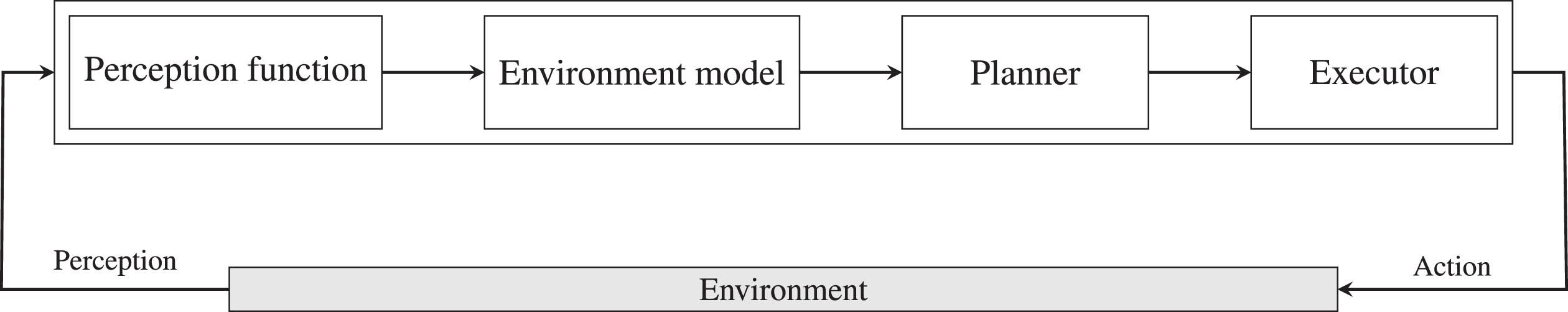
We propose an agent architecture (Fig. 1) that wraps up the learning, planning, and acting components, for an agent accomplishing tasks in an unknown environment. The agent perceives the environment through its sensors; we refer to the perceptual input of the agent as perception. The perception function maps a perception into symbols (i.e. objects and ground atoms) and anchors attributes to the objects (e.g. position, size, visual features, etc.). The output of the perception function is used to build (e.g. by introducing newly discovered objects and their attributes) and update the environment model (e.g. by revising the value of a known object attribute). In particular, the environment model is composed of a symbolic model of the environment, a symbolic state of the agent, and the anchors associated with the symbolic state objects. The symbolic model of the environment describes the environment dynamics, i.e., how the environment evolves when the agent executes actions. The planner takes as input a planning problem composed of: a symbolic model of the environment, an agent symbolic state, and a goal specified by a first-order formula. The planner outputs a plan, if it exists, that is a solution to the planning problem. The executor takes as input the first symbolic action of the plan, returned by the planner, and compiles the symbolic action into a sequence of low-level actions executable by the agent’s actuators.

Fig. 1

Agent environment interface.

Learning the Perception Function. A common assumption in symbolic planning is that the agent perceives the world at the symbolic level, e.g. it does not perceive its position through a GPS sensor, but directly perceives the fact that it is at a particular location, such as “my location is Rome”. Therefore, for applying symbolic planning in a real-world scenario, an agent needs to link the (low-level) perceptions provided by its sensors with symbolic (high-level) observations. A possible approach consists of learning the mapping between continuous and symbolic observations. We refer to the function mapping perceptions into symbols as the perception function. There exists a research area studying this mapping between symbols and their continuous features, which is called perceptual anchoring [8]. In particular, perceptual anchoring is the process of creating and maintaining the correspondence between symbols and perceptions that refer to the same physical objects. In this work, we aim to learn a perception function mapping elements of a perception space into symbolic states. For example, the perception space could be the set of RGB images given by a camera, and a symbolic state may be the set of objects detected in each image together with the predicates representing object properties (e.g. an object box₀ and the ground atom small(box₀)). The perception function can be learned by training supervised models or by end-to-end training of deep reinforcement learning models, which are offline approaches, since they require an input dataset. A still open challenge is how to learn the perception function online, by interacting with the environment. For example, consider a deep learning model predicting the property isOpen for objects of type box. Instead of providing an agent with a pre-trained deep learning model, an agent should interact with a box (e.g. by opening/closing it) in order to learn what an open/closed box looks like, and consequently learn the perception function associated with the isOpen predicate online.

Learning to Act. When an agent computes a symbolic plan, i.e. a sequence of symbolic actions, generally it cannot directly execute the symbolic actions through its actuators. Therefore, the agent needs to compile each high-level symbolic action into low-level control actions. For example, consider a robotic agent that can execute some navigation actions such as moving forward of a number of centimeters or rotating of a number of degrees. Suppose that the agent’s goal is being close to an object of type box, and that the symbolic plan consists of the single high-level action goCloseTo(box₀). The agent cannot directly execute the action goCloseTo(box₀), but it rather needs to compile it into a sequence of low-level navigation actions executable by its actuators. Therefore, we can define an execution function that associates to each high-level action a sequence of low-level actions executable by the agent. Learning the execution function is very challenging when dealing with robotic agents that acts in the real world. The majority of existing approaches tackle this problem by using reinforcement learning or hard-coded solutions (see Section 2). In this work, we do not focus on the problem of learning the execution function online.

Learning the Environment Model. Symbolic planning domains are also referred to as action models. The manual specification of action models is often an inaccurate, time-consuming, and error-prone task. Therefore, the automated learning of action models is widely recognized as a key and compelling challenge to overcome these difficulties. A large number of approaches (see Section 2) tackle the problem of learning action models offline, i.e. from an input set of plan traces. A plan trace is a trajectory in the state space generated by executing a plan, and is composed of the visited states and executed actions in the trajectory. These approaches have different assumptions on the correctness and observability of states and actions in the trajectory.

Few approaches focus on the problem of learning action models online, while executing actions. In the online setting, there is the additional complexity of generating the plan trace. The actions executed for generating a plan trace can be selected randomly, or by an oracle (e.g. a human). Alternatively, they can be selected by the planning itself, i.e., by solving a planning problem where the goal consists of learning a specific part of the action model (e.g. the effects of an action).

Example 1. (Planning, acting and learning agent). A robotic agent equipped with an RGB-D onboard camera and a position sensor is placed in an unknown kitchen and has to put an apple into a box. The agent perceives the RGB-D image of its egocentric view, and detects the objects in the image and their properties through its perception function, which can be a pre-trained deep learning model. The anchors of each object are their visual features extracted from a convolutional neural network that takes as input the RGB image cropped with the object bounding box, and its position which is estimated from the depth camera cropped with the object bounding box. The objects and their properties are used to update the symbolic state of the environment model. The object anchors are used to extend and update the set of anchors in the environment model. In this example, we assume the agent is provided with an input symbolic model of the environment, i.e. a planning domain specified in PDDL. After the environment model has been updated, the agent plans to achieve to goal of putting an apple into a box, then executes the actions in the plan until the goal is achieved. For example, if the first action of the plan is goCloseTo(box₀), the agent uses a path planner for computing a path from its current position to the estimated position of box₀ in the topological map of the environment built online from the depth image while navigating into the environment. Finally, the path plan is translated into a sequence of low-level navigation operations such as moving forward of 20 cm or rotating right of 90 degrees.

In previous work, we focused on the problem of building an extensional representation of a planning domain from sensory data [24], learning action models online [25], exploiting [26] and reusing [7] an input action model for performing tasks in unknown and complex environments. In this work, we address the challenge of using symbolic planning to automate the learning of perception capabilities [27], learning situations where specific portions of the environment can be better perceived, and planning to reach such situations. We evaluate the effectiveness of our approach for learning the perception functions by means of standard machine learning metrics, i.e. the precision and recall, computed on a test set of perceptions. The paper is structured as follows, in Section 2, we discuss related work on the integration of planning, learning and acting. In Section 3, we provide preliminaries about symbolic planning. Then, in Section 4, we define the problem of learning perception capabilities, and in Section 5 we describe our solution proposal. In Section 6, we further extend the proposed solution for learning situations where properties can be better perceived. Afterward, in Section 7, we experimentally evaluate the proposed approach when learning to recognize object properties, and learning the situations where such properties are better perceivable. Finally, in Section 8, we give conclusions and discuss future work.

2 Related work

Several approaches are based on the idea of exploiting automated learning for different planning tasks, like for learning action models, heuristics, plans, or policies. A wide variety of approaches has been proposed for learning action models. Most of the research on learning action models, see, e.g., [1 , 29], does not deal with the problem of learning from real value perceptions. Several approaches have been proposed for addressing the problem of learning planning domains from high-dimensional perceptions (such as RGB images), see, e.g., [2 , 28]. In these approaches, the symbolic planning domain is derived by offline pre-training, and the mapping between perceptions and the symbolic model is fixed, while we learn/adapt this mapping online. We share some similarities with the works on planning by reinforcement learning [39], since we learn by interacting with a (simulated) environment, and especially with the work on deep reinforcement learning [31, 32], which dynamically trains a deep neural network by interacting with the environment. However, deep reinforcement learning focuses on learning policies and perceptions are mapped into state embeddings that cannot be easily mapped into human comprehensible symbolic states. In general, while all the aforementioned works address the problem of using learning techniques for planning, we focus on using planning techniques for learning online and automatically to recognize object properties from low-level high dimensional data.

We share a similar motivation of the research on interactive perception, see [5] for a comprehensive survey, and especially the work in this area to learn properties of objects, see, e.g., [33]. However, most of this work has the objective to integrate acting and learning, and to study the relation between action and sensory response. We instead address the challenge of building autonomous systems with planning capabilities that can automate the training and learning process.

The work by [40] proposes an approach for learning the predicates associated with action effects. They learn action effects by clustering hand-crafted visual features of the manipulated objects, extracted from the continuous observations obtained after executing the actions. However, the learned predicates lack of interpretation, which must be given by a human. On the contrary, our approach learns predicates whose semantic is well-defined a priori and comprehensible by a human. Furthermore, they focus on learning the effects of a single action (i.e., stacking two blocks) in a fully observable environment using ground truth object detection. Our approach learns predicates corresponding to the effects of several actions in partially observable environments, and using a noisy object detector.

In [23], they propose a method for learning a symbolic planning domain assuming the low-level environment state is provided as input. In the work by [23], the semantic of a symbolic state is defined in terms of associated low-level states. Interestingly, the proposed method can learn a symbolic planning domain online by interacting with the environment, i.e. by learning the initiation and effects set of the options executable by the agent. Differently from our work, they assume a structured (though low-level) representation of the environment states is given, the dimension in terms of low-level state variables is fixed a priori, and the low-level states are fully observable. Furthermore, when learning the environment model online, they do not exploit symbolic planning for guiding the search toward informative states. This latter limitation is overcome in the work by [38], where they propose an approach, based on [23], that additionally learns new low-level skills and exploits symbolic reasoning for guiding the environment exploration, according to the intrinsic motivation paradigm.

The approach by [30] learns to map images into the truth values of symbolic predicates. Differently from us, their approach is offline and requires the sequence of images labeled with actions, while our approach plans for generating this sequence online. We share the idea of learning state representations through interaction with [35], where they learn visual representations of an environment by manipulating objects on a table. Notably, they learn the visual representation in an unsupervised way, through a convolutional neural network trained on a dataset generated by interacting with objects. However, the learned representations lack of interpretation and are not suitable for applying symbolic planning. Moreover, none of the above-mentioned methods consider the problem of estimating the quality of the obtained perception model under different conditions to discriminate when perception is trustable. In this work, we also deal with this problem.

3 Background

Let 𝒫 be a set of first-order predicates, 𝒪 a set of operators, 𝒱 a set of variables (also called parameters), and 𝒞 a set of constants. Predicates and operators of arity n are called n-ary predicates and n-ary operators. We use 𝒫 (𝒱) to denote the set of atoms P (x₁, …, x_m), where x_i ∈ 𝒱 and P∈ 𝒫. For instance, if 𝒫 contains the single binary predicate on, and 𝒱 = 〈x₁, x₂, x₃〉. Then, 𝒫 (𝒱) = {on (x_i, x_j) | 1 ≤ i, j ≤ 3}. Similarly, we use 𝒫 (𝒞) to denote the set of atoms obtained by grounding 𝒫 (𝒱) with the constants in 𝒞.

Definition 1. [Lifted action schema] A lifted action schema for an n-ary operator name op ∈ 𝒪 on the set of predicates 𝒫 is a tuple 〈param (op) , ≺ (op) , ^eff+ (op) , ^eff - (op) 〉, where param (op) ⊆ 𝒱, ≺ (op), ^eff+ (op), and ^eff - (op) are three sets of atoms in 𝒫 (param (op)).

Essentially, ≺ (op), ^eff+ (op), and ^eff - (op) represent the preconditions, positive, and negative effects of operator op. Without loss of generality, we assume that operators have no negative precondition.

Definition 2. [Ground action] The ground action a = op (c₁, …, c_n) of an n-ary operator name op ∈ 𝒪 w.r.t. the constants c₁, …, c_n is the triple 〈 ≺ (a) , ^eff+ (a) , ^eff - (a) 〉, where ≺ (a) (resp. ^eff+ (a), ^eff - (a)) is obtained by replacing the i-th parameter of param (op) in ≺ (op) (resp. ^eff+ (op), ^eff - (op)) with c_i.

We use the term lifted, as the opposite of grounded, to refer to expressions and actions where constants have been replaced with parameters.

Definition 3. [Planning domain] A planning domain $M$ is a triple $〈 P, O, H 〉$ where $P$ is a set of predicates, $O$ is a set of operator names with their arity and, for every $op \in O$ , $H$ is a function mapping an operator name op into a lifted action schema.

Definition 4. [Finite-State Machine of a planning domain] The Finite-State Machine (FSM) of a planning domain $M = 〈 P, O, H 〉$ for the set $C$ of constants is the triple $M (C) = 〈 S, A, δ 〉$ where $S = 2^{P (C)}$ is the set of all possible subsets of facts; $A$ is the set of all possible ground actions of each n-ary operator name in $O$ on any n-tuple of constants in $C$ ; $δ \subseteq S \times A \times S$ is a transition relation such that (s, a, s′) ∈ δ if pre (a) ⊆ s and s′ = s ∪ eff⁺ (a) \ eff^- (a).

$M$ is a deterministic planning domain if, given a set $C$ of constants, the transition function δ of $M (C)$ is deterministic, i.e., $\forall (s_{i - 1}, a_{i}, s_{i}) \in δ, ∄ (s_{i - 1}, a_{i}, s_{i}^{'}) \in δ$ where $s_{i} \neq s_{i}^{'}$ . Similarly, $M$ is a discrete planning domain if δ of $M (C)$ is discrete, i.e, the number of elements in the domain $S \times A$ is finite.

Given a set of constants $C$ , a planning domain $M$ can be represented explicitly by $M (C)$ or implicitly by $M$ itself. Indeed, $M (C)$ can be obtained by instantiating $M$ with $C$ , i.e., $A$ can be obtained by grounding the lifted action schemas in $M$ with $C$ , similarly $2^{P (C)}$ can be obtained by grounding the predicates in $P$ with $C$ . Notice that $M$ is a more compact and general representation, since it does not require to explicitly enumerate all possible states and transitions of $M (C)$ , and it can be instantiated with different sets of constants.

Definition 5. [Planning problem] A planning problem is a tuple $〈 M, C, s_{0}, G 〉$ where M is an action model, $C$ is a (possibly empty) set of constants, $s_{0} \subseteq P (C)$ is the initial state, and $G$ is a first-order formula over $P$ , $V$ and $C$ .

Definition 6. [Plan] A plan for a planning problem $〈 M, C, s_{0}, G 〉$ is a sequence 〈op₁(c₁), …, op_n(c_n)〉 such that there is a sequence 〈s₁, …, s_n〉 of subsets of $P (C)$ (aka states), such that for every 0 ≤ i < n, pre (op_i(c_i)) ⊆ s_i, s_i = s_i-1 ∪ eff⁺ (op_i(c_i)) \ eff^- (op_i(c_i)), and $s_{n} ⊨ G$ .

A state s_n ∈ S is reachable from a state s₀ ∈ S in $M (C)$ if there is a plan 〈a₁, …, a_n〉 such that (s_i-1, a_i, s_i) ∈ δ for i = 1 … n.

Notice that our definition of planning problem allows to express the first-order goal formula $G$ . We say that a state $s ⊨ G$ iff $⋀_{p (c) \in s} p (c) \land ⋀_{p (c) \in P (C) \ s} \neg p (c) ⊨ G$ , under the assumption that all the elements of the problem are in $C$ .

4 Problem definition

We suppose that the agent operates in a partially observable environment $E = (S_{E}, A_{E}, δ_{E}, O_{E}, σ)$ , modeled by a non-deterministic automaton $(S_{E}, A_{E}, δ_{E})$ , where $S_{E}$ is a set of environment states, $A_{E}$ a set of agent “low-level” actions executable in $E$ , and $δ_{E} \subseteq S_{E} \times A_{E} \times S_{E}$ is a transition relation; the set of environment observations is denoted by $O_{E}$ , and $σ : S_{E} {→O}_{E}$ is a deterministic observation function.

Example 2. Suppose that there is an agent in a room that needs to see the picture on the wall in front of it, but its view is occluded by a circular object. The agent can move so that the object only partially occlude the picture. Moreover, the agent can turn on or off the light in the room. The set $O_{E}$ of environment observations is composed by images of size w × h; in Fig. 2 we show some examples of observations.

Fig. 2

Examples of environment observations where a digit three is displayed on the wall. The light is off in observation (a), and on in observations (b)–(e); whereas the occluding object is in the center of the observation (b), on the edge in (c), and in a corner in (d) and (e).

We model the agent by $Ag = 〈 M_{Ag} (C), {ex}_{Ag}, f_{Ag} 〉,$ where $C$ is a set of constants (i.e. objects in the environment), $M_{Ag} (C) = (S_{Ag}, A_{Ag}, δ_{Ag})$ is a finite-state machine represented by a set S_Ag of agent states, a set A_Ag of agent “high-level” actions, and a transition relation δ_Ag ⊆ S_Ag_timesAAg_timesSAg. The finite-state machine $M_{Ag} (C)$ represents the symbolic representation of the environment internally adopted by the agent. We differentiate among S_Ag and $S_{E}$ since the internal agent state may abstract away portions of the state of the environment that are not relevant for the agent goals.

Furthermore, the agent can perform the high-level actions in A_Ag by executing the corresponding low-level actions in $A_{E}$ . The correspondence between high and low level actions is represented by the function ex_Ag, which associates to each pair (s, a) ∈ S_Ag_×AAg a program ex_Ag (s, a) of actions in $A_{E}$ executable in $E$ , such as, e.g., in hierarchical task networks [12]. The environment state obtained by executing ex_Ag (s, a) is nondeterministic, since the environment is nondeterministic. The problem of learning ex_Ag goes out of the scope of this paper, see for instance [11]. However, notice that we do not assume the execution of the actions leads to the symbolic state predicted by the planning domain. For example, by executing the action Go_Close_To(c), an agent may reach a state where it is not close enough to the object c, i.e. the predicate Close_To(c) is false, even if it is a positive effect of Go_Close_To(c). Furthermore, executing a symbolic action may produce effects that are not in the planning domain. For instance, an object property may become true after executing a symbolic action involving the object, even though it is not a positive effect of such an action in the planning domain. Therefore, the agent must check if its plan is valid when executing the plan actions, and possibly react to unexpected situations, e.g., by replanning.

Finally, the agent is associated with a perception function $f_{Ag} : O_{E} \to \Pr (S_{Ag})$ that gives a probability distribution f_Ag (s ∣ o) over the states s ∈ S_Ag given an observation o in $O_{E}$ .

We suppose that an agent $Ag = 〈 M_{Ag} (C), f_{Ag}, {ex}_{Ag} 〉$ is placed at a random position in a new environment (i.e. $C = \emptyset$ ); we represent and initialize f_Ag with the following components: (i) a pre-trained object detector f_o; (ii) an untrained neural network f_t,p for predicting the property p of the objects of type t, for a subset of pairs (t, p) of interest.

Given a perception (e.g., RGB-D image), the object detector returns a set of objects with their types, where the set of object types is shared with the planning domain. Each object detected in the perception is linked with a set of numeric features (e.g. estimated position, bounding box, etc.), which constitute the anchors of the object [8]. The features of the detected objects are compared with the ones of the objects already known by the agent, i.e., those belonging to the current set of constants $C$ . When the features of a detected object match (to a certain degree) the features of a known object $c \in C$ , then the features of c are updated with the detected object ones. For example, the position of c is updated by averaging its known position with the position of the matching object. Otherwise, $C$ is extended with a new constant c′ anchored to the features of the detected object, and the type t (c′) is asserted in the planning domain, where t is the object type returned by the object detector.

For every object c of type t and for every property p that applies to objects of type t, a classifier f_t,p predicts if the property p holds for c, i.e., if p (c) is true. It is worth noting that a property is not applicable to all object types, e.g., it does not make sense to check if a laptop is filled or empty. f_t,p can be implemented by an hard-coded function or a machine learning model trained, e.g., in a supervised way. For example, the classifier of property Close_To applied to an object, indicating whether the agent is close to the object, can be defined by a threshold on the distance among the object position and the agent one. Whereas some properties, such as Is_Open, can be predicted by means of a neural network, which given an object image returns the probability of the property being true for the object.

We focus on the problem of training f_t,p in an online way for some pair (t, p) of interest; we devise a method to autonomously produce symbolic plans for collecting a training set T_t,p, and exploit T_t,p for training the perception function f_t,p. The set T_t,p consists of tuples (c, v), where c is a constant identifying an object of type t and its anchors (e.g., the object visual features) and v is the truth value of p (c). It is worth noting that T_t,p can contain wrong labels, since it is automatically generated by interacting with the environment.

We assess the efficacy of our method by measuring the precision and recall of each f_t,p w.r.t. a ground truth dataset independently collected by the agent.

5 Method

To describe the proposed method, we adopt a simple example. Suppose an agent needs to learn to classify property Is_Turned_On for objects of type Tv, such an agent can act as follows: (i) look for an object tv₀ of type Tv; (ii) turn tv₀ on to make true property Is_Turned_On(tv₀); (iii) take pictures of tv₀ from different points of view, and label them as positive examples for Is_Turned_On. Similarly, the agent can produce negative examples for Is_Turned_On by executing action Turn_Off(tv₀) and taking pictures of tv₀.

The previous behaviour should be autonomously planned and executed by the agent for a given pair (t, p), where p is a learnable property applicable to objects of type t. To this aim, we extend the planning domain of the agent such that, given the synthesized high-level goal of learning p for t, the procedure of collecting training data for f_t,p is automatically generated by a symbolic planner, and executed by the agent. We assume that, for every pair (t, p) to be learned, the agent is given the information that there is at least a planning domain operator that makes p true for objects of type t, and an operator that makes p false.

5.1 Extended planning domain for learning

We extend the planning domain M with the capability of expressing facts about its properties and types, i.e., we introduce in M the following meta predicates and names.

Names for types and properties. For every object type $t \in P$ (e.g., Box), we add a new constant ‘t’ (e.g., ‘box’) 1 . Similarly, for each object property $p \in P$ (e.g., Is_Open), we add two new constants ‘p’ and ‘not_ p’ (e.g., ‘is_open’ and ‘not_is_open’).

Epistemic predicates. We introduce new predicates in $P$ indicating that an agent knows/believes a certain property hold for an object in a given state. The binary predicate Known(o,‘p’) (resp. Known(o, ‘ not _ p’)) states that the agent knows that the object o has (resp. does not have) the property p. The atom Known(x,‘p’) is automatically added to the positive (resp. negative) effects of all the actions that have p (x) in their positive (resp. negative) effects; similarly, the atom Known(x,‘not_p’) is automatically added to the positive (resp. negative) effects of all the actions that have p (x) in their negative (resp. positive) effects. For example, the atoms Known(x, ‘is_turned_on’) and Known(x, ‘not_is_turned_on’) are added to the positive and negative effects of Turn_On(x), respectively. Similarly, the atoms Known(x, ‘is_turned_on’) and Known(x, ‘not_is_turned_on’) are respectively added to the negative and positive effects of Turn_Off(x).

Predicates and operators for observations. We extend the planning domain by introducing operators for observing, exploring, and learning (see Table 1). In particular, we add an operator Observe(o, t, p), whose input argument are an object o, a type t, and a property p. When Observe(o, t, p) is executed, the training dataset T_t,p is extended with images of object o taken from different point of views. To prevent the agent from repeatedly observing object o for the property p, we add the atom Viewed(o, p) as a positive effect and ¬Viewed (o, p) as a precondition of Observe(o, t, p).

Table 1
Action schemas for Explore_for, Observe and Train

Explore_for(t, p)

pre: ∀x (Known (x, t, p) → Viewed (x, t, p))

¬ Sufficient_Obs(t, p)

eff⁺: Explored_for(t)

Observe(o, t, p):

pre: ¬Viewed(o, t, p)

Closed_To(o)

Known(o, t, p)

eff⁺: Sufficient_Obs(t, p)

Viewed(o, t, p)

Train(t, p, q):

pre Sufficient_Obs(t, p)

Sufficient_Obs(t, q)

eff⁺: Learned(t, p, q)

Moreover, the positive effects of Observe(o, t, p) involve the atom Sufficient_Obs(t, p), which is true when the agent has collected enough observations for learning property p applied to objects of type t.

When the agent executes Observe(o, t, p) but do not collect enough observations for learning p applied to objects of type t, the atom Sufficient_Obs(t, p) does not become true, contrarily to what is predicted by the planning domain, and the agent needs to plan for further collecting observations.

Predicates and operators for exploration. We extend the planning domain with the operator Explore_for(t, p) that looks for new objects of type t by exploring the environment. The operator Explore_for(t, p) can be executed when all the known objects of type t have been observed for learning the property p. Specifically, the precondition of Explore_for(t, p) is ∀x (Knows (x, t, p) → Viewed (x, t, p)). Indeed, when the agent finds a new object, then it creates a corresponding new object o in the planning domain, and becomes aware that it can observe properties of o. The positive effects of Explore_for(t, p) involve the atom Explored_for(t), which indicates that the agent has (even partially) explored the environment, looking for new objects of type t. However, executing Explore_for(t, p) does not make Explore_for(t, p) true until the environment has been fully explored, or a maximum number of iterations has been reached.

Predicates and operators for learning. We add to the planning domain the atom Learned(t, p, not _ p), which indicates whether the agent has learned to recognize property p for objects of type t, i.e., if the agent has trained f_t,p. We extend the planning domain with the operator Train(t, p, q). The execution of Train(t, p, q) consists of training the network f_t,p with a set T_t,p of positive examples and a set T_t,q of negative ones. The preconditions of Train(t, p, q) contain the atoms Sufficient_Obs(t, p) and Sufficient_Obs(t, q) that guarantee the agent has collected a sufficient number of positive and negative examples, which are necessary for training f_t,p. The set of positive effects of Train(t, p, q) includes only the atom Learned(t, p, q).

Specifying the goal formula. The goal formula g for learning a property p for an object type t is defined in the extended planning domain as follows:

$g = Learned (t, p, not_p) \lor Explored_for (t) .$ (1)

For example, when an agent aims to learn the property Turned_On applied to objects of type Tv, then g = Learned (‘tv’, ‘turned _ on’, ‘not _ turned _ on’) ∨Explored _ for (‘tv’). Let tv₀ denote an object of type Tv where both Viewed(tv₀,‘tv’,‘is_turned_on’) and Viewed(tv₀, ‘tv’,‘not_is_turned_on’) are false, then the goal can be achieved by executing the plan:

Go_Close_To(tv₀)

Turn_On(tv₀)

Observe(tv₀, ‘tv’,‘turned_on’)

Turn_Off(tv₀)

Observe(tv₀,‘tv’, ‘not_turned_on’)

Train(‘tv’, ‘turned_on’,‘ not_turned_on’).

After executing all the plan actions but the last one, suppose that the agent has not gathered enough training data for ‘turned_on’ and ‘not_turned_on’, then the atoms Sufficient_Obs(‘tv’, ‘turned_on’) and Sufficient_Obs(‘tv’,‘not_turned_on’) are false, and therefore the last plan action is not executable. In this situation, the agent needs to replan for finding another tv which has not yet been observed.

Finally, it is worth noting that when the agent has observed all the known objects of type Tv for the property Turned_On, then the formula ∀xKnown(x,‘tv’, ‘turned_on’)→Viewed(x, ‘tv’,‘turned_on’) is satisfied, and the goal is reachable by producing a plan that satisfies Explored_for(‘tv’), i.e., by executing the action Explore_For(‘tv’,‘turned_on’), which explores the environment for new objects of type ‘tv’.

Algorithm 1 Plan to Learn Object Properties

Input: $Ag = 〈 M_{Ag} (C), {ex}_{Ag}, f_{Ag} 〉$

Input: g = ⋀ _(t,p)∈TP (Learned(t,p)∨ Explored_For(t))

1: extend M with actions and predicates for learning

2: $C \leftarrow$ names for types and properties in $P$

3: s← ∅

4: T_TP ← {T_t,p = ∅ ∣ (t, p) ∈ TP}

5: f_TP ← {f_t,p = randominit . ∣ (t, p) ∈ TP}

6: $π \leftarrow Plan (M (C), s, g)$

7: While π ≠ 〈〉 do

8: op ← Pop (π)

9: s ← s ∪ eff⁺ (op) \ eff^- (op)

10: $C, T_{TP}, f_{TP} \leftarrow Execute (op)$

11: s ← Observe ()

12: $π \leftarrow Plan (M (C), s, g)$

13: end while

5.2 Main control cycle

A procedure of the proposed method is reported in Algorithm 1, where Ag is an input agent and g the goal of learning a set TP of object type-property pairs. Initially, the set $C$ of constants is only composed of the names for object types and properties, and s is the empty state (Lines 2–3). For each pair (t, p) ∈ TP, the set T_t,p is initialized to the empty set, and the neural networks f_t,p are randomly initialized (Lines 4–5). Afterward, on line 6 the agent produces a plan π. As long as the plan π is not empty, (Lines 7–13), firstly the agent selects the first plan action and updates the state s according to the action schema (Line 9). Next, the agent executes the first plan action and updates the set $C$ of constants, the datasets T_t,p, and the neural networks f_t,p (Line 10). It is worth noting that, since the perceived action effects may differ from those specified in the action schema, the agent needs to sense using the not trainable perception functions, and update its current state accordingly (Line 11). Furthermore, since π may become invalid in the updated state, a new plan must be produced (Line 12). The algorithm terminates if either a maximum number of iterations has been performed or the environment has been fully explored. In fact, in such cases, the atom Explored_for(t) is true, and plan π for g is empty.

6 Learning to better perceive

So far we have not considered the problem that object properties are not always perceivable. For example, an agent can perceive whether a mug is empty only by looking inside the mug, or it can perceive if a fridge is empty only when the fridge is opened. In the following, we extend our approach for learning the situations where properties are better perceivable. For the sake of clarity, hereafter we specify the agent state by means of a set of state variables x = (x₁, …, x_n), following the SAS+ formalism [4].

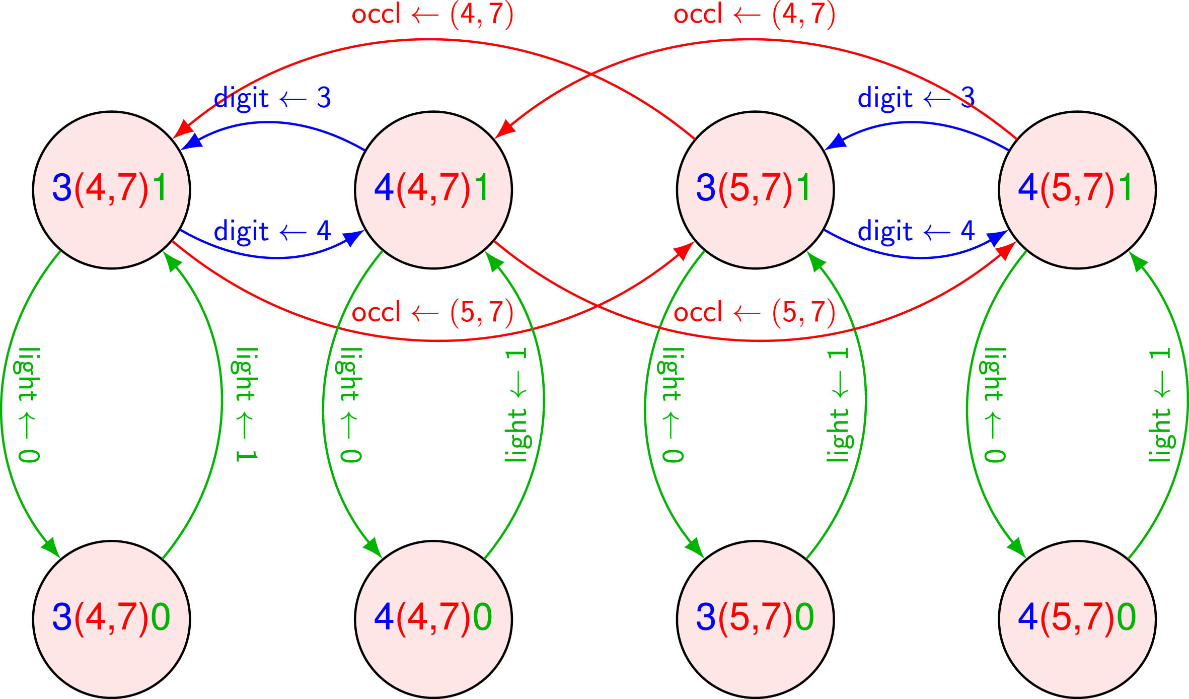
Example 3. (Agent’s transition system) The set S_Ag of agent states in Example 2 can be represented by three state variables: digit that takes values in {0, …, 9}, occl that takes values in {(i, j) ∣0 ≤ i ≤ w, and 0 ≤ j ≤ h}, and light that takes boolean values. For example, the state 3(4,7)0 ∈ S_Ag describes the situation where a picture of digit 3 is on the wall, the occluding object is centered in (4,7), and the light is off. The set A_Ag of agent high-level actions allows to switch on/off the light, change the picture of the digit on the wall, and move the occluding object to a different position. Specifically, for each state variable x ∈ {digit, occl, light}, x ← v is an action effect that assigns to x the value v in the domain of x. We hypothesize that all the actions but switching on/off the light can be only performed when the light is on. A portion of the agent transition system is shown in Fig. 3, where we consider only digits 3 and 4 and an occluding object placed in positions (4, 7) or (5, 7).

Fig. 3

A portion of the agent transition system.

The perception function of the agent can be represented as f_Ag = (f_{x
₁}, …, f_{x
_n}).

Example 4. (Agent perception function) In the previous example, we can model the agent perception function with a perception function for each state variable, i.e., f_Ag = (f_digit, f_occl, f_light), defining f_Ag (s ∣ o) as: $\begin{matrix} (f_{digit} (s_{digit} ∣ o), f_{occl} (s_{occl} ∣ o), f_{light} (s_{light} ∣ o)) \end{matrix}$ where s_x denotes the value of x in state s, for each x ∈ {digit, occl, light}, and o is an observation of s.

We group the variables of the agent state into control variables and observable variables. The values of the control variables are known in every state; on the contrary, the values of the observable variables can be known only in some states. For instance, light belongs to the set of control variables since its value can be known in every state; whereas the value of digit is known only when the light is on, therefore digit is an observable variable. Consequently, not all environment observations can generally provide the agent with sufficient information for discriminating, by means of f_Ag, the observable variables values. In fact, as in the previous example, if the light is off then the environment observations do not allow the agent to discriminate the value of the observable state variable digit by means of f_digit. As a result, to trust a perception function prediction, an agent needs to know (believe) that the environment is in a state where such prediction is sufficiently confident. Therefore, we: (i) extend the agent definition with a subset of states B_Ag⊆_SAg representing the belief state of the environment; (ii) define the perception function confidence in a belief state.

Definition 7. [Confidence in a state] The confidence of the agent perception function f_Ag in a state s∈ S_Ag, denoted by conf (f_Ag, s), is defined as $\frac{1}{| δ_{Ag}^{- 1} (s) |} \sum_{(s^{'}, a) \in δ_{Ag}^{- 1} (s)} E_{o \sim {ex}_{Ag} (s^{'}, a)} f_{Ag} (s ∣ o)$ (2) where $δ_{Ag}^{- 1} (s) = {(s^{'}, a) ∣ (s^{'}, a, s) \in δ_{Ag}}$ .

Definition 8. [Confidence in a belief state] The confidence of the agent perception function f_Ag in a belief state B_Ag⊆ S_Ag is the average of the confidence of f_Ag in each state s ∈ B_Ag.

Intuitively, Equation (2) states that, for every way of reaching s, i.e., for every (s′, a, s) ∈ δ_Ag, $E_{o \sim {ex}_{Ag} (s^{'}, a)}$ f_Ag (s ∣ o) is the expectation of the agent believing to be in s given the observation o acquired after the execution of a in s′. Since the action execution is non-deterministic, the observation o acquired after executing an action is a random variable. The higher the expectation value, the higher the accordance among the abstract model, the perception function and the actual execution of the high-level action a. This expectation is averaged over all possible ways of reaching s.

Let x _–i = v _–i be the assignments to all state variables but x_i. The confidence of f_{x
_i} conditioned on x _–i = v _–i is determined as the confidence of f_Ag in S_{x
_–i=
v
_–i} = {s ∈ S_Ag ∣ s_{x
_j} = v_j ∀ j ≠ i}.

Definition 9. (Viewpoint) A viewpoint with confidence at least t ∈ [0, 1] for a state variable x is a belief state B_Ag ⊆ S_Ag such that conf (f_x, B_Ag) ≥ t.

Example 5. Let f_digit, f_light and f_occl be neural networks trained with labeled observations as those shown in Fig. 2. For example, f_light is trained with a set of observations labeled with 0 that are similar to the first shown in Fig. 2, and a set of observations labeled with 1 that are similar to the remaining observations in Fig. 2 (possibly with the occluding object in different positions and different digits). Similarly, f_occl is trained with observations as (a) and (b) labeled with $(\frac{w}{2}, \frac{h}{2})$ (i.e. the occluding object is placed in the center, though in (a) is not visible), with observations like (c) labeled as $(\frac{w}{2}, h)$ , and with observations similar to (d) and (e) labeled with (w, h) and (w - 4, 4), respectively. It is reasonable to expect that f_light is highly confident in every belief state B, since the visual difference of the observations is evident, regardless of the occluding object and the digit. On the contrary, f_occl will have high confidence only in the belief states where the light is on (i.e, the state variable light has value 1). Finally, the confidence of f_digit will be high when the light is on and the occluding object is in a corner, medium when the object is close to the edges, and low when it is close to the middle. Overall, f_Ag will be highly confident when the light is on, and the occluding object is on a corner, i.e., in the belief state B_corner = {s ∈ S_Ag ∣ s_light = 1 and s_occl ∈ {(0, 0) , (w, 0) , (0, h) , (w, h)}}.

For perceiving the current environment state correctly, an agent needs to know the belief states where the perception function is sufficiently confident. In fact, if f_Ag is highly confident in B_Ag, then the agent can trust f_Ag for deriving its current state from the current observation o of the environment state, e.g., by computing $s^{*} = \underset{s}{argmax} (f_{Ag} (s ∣ o))$ , and obtaining the least ambiguous (total) belief state equal to {s^*}. When, instead, the confidence of f_Ag is low in B_Ag, then observing the environment being in B_Ag does not provide reliable information about the current state of the agent. In such a scenario, the agent needs to find a plan π for reaching a new belief state δ_Ag (π, B_Ag) where f_Ag is sufficiently confident.

Example 6. Consider the environment defined in Example 2(a) with the light off. Suppose the agent wants to know the digit that is on the wall, and its initial belief state comprises the entire set of states S_Ag, i.e. the agent has no belief. Firstly, the agent perceives the black image reported in Fig. 2. Since the confidence of f_light is high in any belief state, then the agent can trust the predictions of f_light. Hence, the prediction of f_light will lead to a belief state S_light=0 = {s ∈ S ∣ s_light=0}. Since in such a belief state the confidence of f_digit is low, then the agent needs to plan for reaching a belief state where f_light is more reliable, i.e., the belief state B_corner as defined in Example 5. To reach B_corner the agent can sequentially execute two actions those effects are light ← 1, and occl ← c with c ∈ {(0, 0) , (0, h) , (w, 0) , (w, h)}. Thus, after the plan execution, the agent will get an observation as the two rightmost pictures in Fig. 2, With this observation, the agent can derive with a high confidence that digit = 3 by means of the perception function f_digit.

We extend our approach to address the following task. Given an agent $Ag = 〈 M_{Ag} (C), B_{Ag}, f_{Ag}, {ex}_{Ag} 〉$ and a state variable x, find a set of viewpoints B₁, …, B_k for x with confidence greater than t, and produce a plan π such that δ_Ag (π, B_Ag) = B_i for some 1 ≤ i ≤ k.

For the sake of presentation, we describe how we extend our approach by assuming that x₁, …, x_n-1 are control variables and only variable x_n is observable. Consequently, the perception function f_{x
_i} for 1 ≤ i < n is highly confident in all belief states, and provides the ground-truth value. It is worth noting that our method is applicable also for different partitions of the state variables in observable and control variables. The agent needs to find the belief states where it can observe the value of x_n by means of f_{x
_n} with sufficiently high confidence. For instance, in Example 4 the agent is given a perception function for every state variable; we assume that the perception function of f_occl, and f_light provide the ground-truth values, while the agent needs to find the belief states where the confidence of f_digit is above a given threshold.

6.1 Estimating the perception confidence

To estimate the confidence of f_{x
_n} in an agent state s ∈S_Ag, the agent can approximate Equation (2). To this aim, the agent needs a set of observations $O_{s} \subseteq O_{E}$ labeled with the value of x_n in s. The set O_s can be obtained by executing a plan for getting into s and collecting observations from the reached environment state. In Example 2, if the agent is in state 4 (4, 7) 1, it can construct the observation set O_3(4,7)1 by executing the action with effect digit ← 3 and adding the observation taken from the resulting state to O_3(4,7)1. In Example 2, when 4 (4, 7) 1 is the agent state, the set of observations O_3(4,7)1 can be obtained by executing the action with effect digit ← 3 and augmenting O_3(4,7)1 with the observation collected from the reached state.

In the following, we tackle the problem of finding a set of belief states ℬ = {B₁, …, B_k} ⊆2^{S
_Ag} where the state variable x_n is observable. To this aim, we could take into account all the belief states derived by assigning the control variables x _-n to every possible value v _-n. In the previous example, the agent could consider the belief states where control variables light and occl are fixed to some values; an example of belief state is S_{light=1,occl=(0,0)} = {0 (0, 0) 1, 1 (0, 0) 1, …, 9 (0, 0) 1}.

For estimating the confidence conf (f_{x
_n}, B_i) in a belief state B_i, the agent computes:

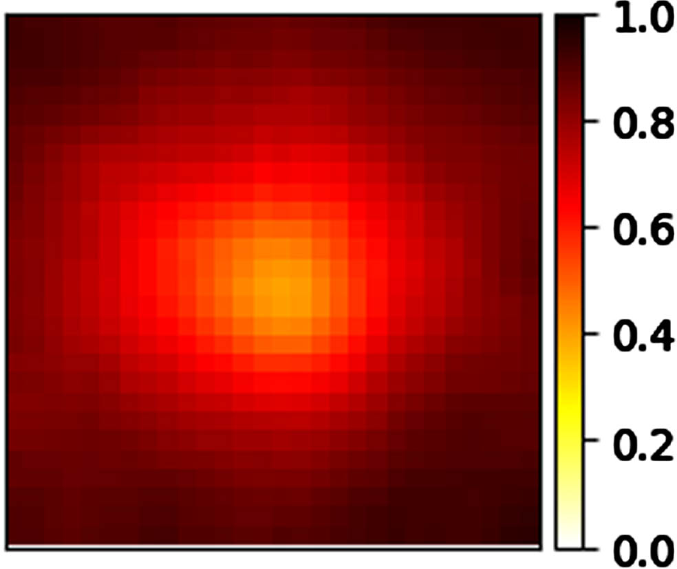
$\frac{1}{| B_{i} |} \sum_{s \in B_{i}} \frac{1}{| O_{s} |} \sum_{o \in O_{s}} f_{x_{n}} (s ∣ o) .$

In Fig. 4, we show the confidence of the perception function (i.e. the neural network) predicting the value of the observable variable digit considered in previous example, where light and occl are control variables. For example, in Fig. 4, the heatmap reports the neural network confidence on images collected in states where light = 1 and the value of occl varies among the image pixel coordinates. More precisely, every heatmap pixel (i, j) shows the network confidence averaged over all images with the occluding circle centered at position (i, j). Not surprisingly, the confidence decreases when the occluding circle is placed in the middle of the image.

Fig. 4

Heatmap of the confidence of the perception function f_digit in our running example.

6.2 Find viewpoints via clustering

The simple methodology reported above cannot be applied when the number of combinations of control variable values is large. In such situation, there is a huge number of states in S_Ag, and therefore it is not feasible to collect a set of observations for every state in S_Ag. Moreover, the set of belief states obtained by fixing the control variable values is exponentially large w.r.t. the number of control variable values. To cope with the problem of collecting a set of observations for every state in S_Ag, we acquire observations from a subset of states, which is a good representative sample for the domain of the control variables. Next, we cluster the acquired observations into a set of belief states, where every cluster is associated with a different belief state, and we select the clusters where the confidence of the perception function is sufficiently high. For clustering, we assume numerical control variable values (e.g., light on/off is encoded by light equal to 1/0), and we denote by dist ( v , v ′) the distance measure between a pair of control variable values v , v ′. We detail such a procedure in Algorithm 2.

Firstly (Lines 2–11), for each possible value v_n of the observable variable x_n, the agent collects the confidence y of observing v_n from m states where x_n = v_n. Each y is associated with the value v _-n of the control variables in the state where x_n has been observed. For this purpose, the agent sequentially samples m assignments v _-n of the control variables x _-n (Line 4); next, it computes a plan for getting into the state x = ( v _-n, v_n) from its current belief state B_Ag (Line 5). After executing the plan, the agent observes the reached environment state (Line 6), and, on Line 7, computes the confidence y = f_{x
_n} (v_n ∣ o) of observing v_n. Finally, the agent updates its belief state B_Ag on Line 9. It is worth noting that f_{x
_n} is learned from observations collected online. In fact, for each f_{x
_n}, there is a planning domain action for training the neural network associated with f_{x
_n} (Line 6).

In the second part of the algorithm (Lines 13–17), for every partial assignment v _-n in F, the agent computes the average confidence y^* of the predictions performed from the neighbor states N ( v _-n), i.e., from states such that $dist (v_{- n}, v_{- n}^{'}) \leq r$ , where r ∈ ^R+ is a given threshold.

In the last part of the algorithm (Lines 18–25), the agent constructs a set of belief states ℬ based on F^*. The elements of F^* are clustered in the sets C₁, …, C_k (in our experiments we applied the K-mean algorithm). The agent constructs the set $C$ of clusters with an average confidence higher than a given threshold t. For every cluster in $C$ , the agent derives the cluster centroid c _i by averaging the control variable values v _-n (Line 23). Then, the agent derives the belief state B_i associated with the cluster C_i by choosing the states in S_Ag whose control variables distance from c _i is less than threshold r (Line 23). Finally, the set ℬ of belief states is augmented with B_i.

Algorithm 2 Find Belief States

Input: $Ag = 〈 M_{Ag} (C), B_{Ag}, {ex}_{Ag}, f_{Ag} 〉$

Input:t ∈ [0, 1]: confidence threshold

Input:r ∈ ^R+: belief state radius

Input:m: number of sampled values for x_n

1: F← ∅

2: for v_n ∈ Dom (x_n) do

3: for i ∈ {1, …, m} do

4: v _-n← uniformly sample values for x _-n

5: π←Plan( $M_{Ag}, B_{Ag}, S_{x = (v_{- n}, v_{n})}$ )

6: o ← ex_Ag (π)

7: y ← f_{x
_n} (v_n ∣ o)

8: F ← append (F, 〈 v _-n, y〉)

9: B_Ag ← δ_Ag (π, B_Ag)

10: end for

11: end for

12: F^*← ∅

13: for ( v _-n, y) ∈ F do

14: $N (v_{- n}) \leftarrow {(v_{- n}^{'}, y^{'}) \in F ∣ dist (v_{- n}^{'}, v_{- n}) \leq r}$

15: $y^{*} \leftarrow \frac{1}{| N (v_{- n}) |} \sum_{(v_{- n}^{'}, y^{'}) \in N (v_{- n})} y^{'}$

16: F^* ← append (F^*, 〈 v _-n, y^*〉)

17: end for

18: C₁, … C_k ← Clustering (F^*)

19: $C \leftarrow {C_{i} ∣ \frac{1}{| C_{i} |} \sum_{〈 v_{- n}, y^{*} 〉 \in C_{i}} y^{*} > t}$

20: ℬ← ∅

21: for $C_{i} \in C$ do

22: $c_{i} \leftarrow \frac{1}{| C_{i} |} \sum_{〈 v_{- n}, y^{*} 〉 \in C_{i}} v_{- n}$

23: B_i ← {s_inSAg ∣ dist (s_{x

_-n}, c _i) ≤ r}

24: ℬ ← ℬ ∪ {B_i}

25: end for

26: return ℬ

6.3 Planning to reach a belief state

To perceive the observable variable x_n, the agent produces and executes a plan π from its current belief state for reaching a belief state in ℬ, which is returned by Algorithm 2. For this purpose, we adopt symbolic (PDDL) planning, hence the agent’s automaton $M_{Ag}$ is specified as a planning domain. The planning domain specification comprises a set of operators for changing the values of state variables x₁, …, x_n. For instance, in the previous example, the agent can modify the value of control variable light by executing the action with effect light ← 1.

For the observable variable x_n, we introduce a predicate known _ xn in the planning domain, for indicating that the agent knows the value v_n of x_n. For every belief state B_i ∈ ℬ, and partial assignment v _-n ∈ s for all s ∈ B_i, we extend the planning domain with an action observe _ xn ( v _-n) with preconditions x_i = v_i for all 1 ≤ i < n, and positive effect known _ xn. Finally, we define a planning problem where, in the initial state, x_i = v_i with 1 ≤ i < n and v_i ∈ s for all s ∈ B_Ag; and the goal is known _ xn.

Example 7. Let x_n = digit, $B_{Ag} = S_{light = 0, occl = (\frac{w}{2}, \frac{h}{2})}$ ,and ℬ = {S_{light=1,occl=(0,0)}, S_{light=1,occl=(w,h)}}. Therefore, the planning domain is extended with actions observe _ digit (1, (0, 0)) and observe _ digit (1, (w, h)). The action preconditions are {light = 1, occl = (0, 0)} and {light = 1, occl = (w, h)}, respectively; the action (positive) effect is known _ digit (). In the initial state of the planning problem $light = 0, occl = (\frac{w}{2}, \frac{h}{2})$ , and the goal is known _ digit ().

7 Experimental analysis

We firstly focus on the problem of planning for learning to recognize object properties, and then on the problem of learning the belief states where object properties are better perceivable, and plan to reach such states.

7.1 Learning to recognize object properties

We evaluate the performance of our approach for collecting a dataset and training neural networks for predicting the four properties Is_Open, Dirty, Toggled, and Filled on 32 object types, resulting in 38 pairs (t, p), since not all properties can be applied to every object type.

Simulated environment. We experiment with our approach in the ITHOR [21] photo-realistic simulator of four types of indoor environments: kitchens, living-rooms, bedrooms, and bathrooms. We perform a set of experiments in the ITHOR [21] photo-realistic simulator comprising four types of indoor environments: bedrooms, bathrooms, kitchens and living-rooms. ITHOR simulates a mobile robot that can navigate the environment and interact with environment objects by modifying their properties (e.g., turning on a tv, opening a box). The agent is provided with two sensors: an odometry sensor and an RGB-D camera. We grouped the 120 environments provided by ITHOR into 80 environments for training, 20 for validation, and 20 for testing. Testing environments are evenly distributed among the 4 environment types.

Object detector. As an object detector f_o, we adopted the YoloV5 model [13], which takes as input an RGB image and outputs the bounding boxes detected in the image and the predicted object types. To train f_o, we generated a training (resp. validation) set by randomly navigating in the training (resp. validation) environments, and labeled the observations with the ground truth object types and bounding boxes provided by ITHOR. The training and validation sets comprise 115 object types and are composed by 259859 and 56190 labeled observations, respectively. To validate the object detector, we run the genetic algorithm used in [13] 300 times (with 10 epochs for each run).

Property predictors. We encode the perception functions f_t,p, for predicting properties, as a ResNet-18 model [17] with an additional fully connected linear layer as output, which takes as input the RGB image of the object and returns the probability of property p applied to the object being true. We consider p applied to the object being true if the probability is higher than a threshold (set to 0.5 in our experiments).

Evaluation metrics and ground truth. We evaluate every f_t,p by means of the metrics precision and recall against a test set G_t,p, built by randomly navigating the 20 testing environments and using the ground-truth information provided by ITHOR. In particular, for property Is_Open we generated a test set with 8751 examples, 2512 for Toggled, 1310 for Filled, and 3304 for Dirty. Notice that the size of the test set for property Is_Open is higher than for other properties since Is_Open can be applied to a higher number of object types than other properties.

We run our approach in every testing environment for collecting online a training set T_t,p and training the neural network associated with f_t,p. At every run, the agent is placed in a random position of the environment and performs 2000 low-level operations (e.g., move forward of 30 cm).

For investigating how the object detector errors affect the performance, we devised two variants of our approach: ND (Noisy Detections) and GTD (Ground-Truth Detections). In both variants, the agent collects a training set T_t,p in a single environment, which is then used for training f_t,p. Then, f_t,p is evaluated on the test set G_t,p previously generated in the same environment. For ND variant, the agent is given a pre-trained object detector f_o; whereas for GTD variant the agent is given a perfect f_o, i.e., the ground-truth object detections provided by ITHOR. In both variants, every neural network f_t,p is trained for 10 epochs with 1e^-4 learning rate, and other hyperparameters are assigned the default values provided by PyTorch1.9 [34].

Experimental results. For every learned property, in Table 2 we compare the performance of ND and GTD variants. Specifically, Table 2 reports the object type, the number of labeled observations collected in the training and test sets, respectively T_t,p and G_t,p, the metrics precision and recall averaged over all 20 testing environments. Notice that the size of the test set can vary among ND and GTD, since we remove from the test set the object types that are missing in the training set, i.e., the object types that have not been observed by the agent. Indeed, we evaluate the learning performance considering the object types that the agent actually manipulated and observed. Furthermore, some specific object types (e.g., desktop and showerhead in Table 2) are never recognized by the object detector, thus they are not in the training set, and they are assigned the ‘-’ value in Table 2.

Table 2
Size of the ground truth test set G_t,p, the generated training set T_t,p, and performance in terms of precision and recall on the 38 type-property pairs

Size of G_t,p Size of T_t,p Precision Recall

Object type ND GTD ND GTD ND GTD ND GTD

Dirty

Bed 564 564 1502 671 0.95 0.57 0.43 0.61

Bowl 280 280 383 1027 0.67 0.98 0.81 0.73

Cloth 96 210 61 503 0.93 0.95 0.78 0.70

Cup 96 262 146 986 0.63 0.99 0.95 0.54

Mirror 654 678 2490 3100 0.91 0.90 0.68 0.80

Mug 230 432 225 1367 0.88 0.94 0.42 0.74

Pan 140 200 20 476 0.76 0.99 0.87 0.79

Plate 166 406 47 1304 0.61 0.97 0.97 0.77

Pot 210 272 51 929 0.76 0.99 0.91 0.98

Weighted avg - - - - 0.84 0.89 0.68 0.74

Filled

Bottle 22 22 78 150 0.65 0 1.00 0

Bowl 328 256 390 1091 0.64 1.00 0.73 0.77

Cup 116 286 200 1028 0.92 0.90 0.56 0.68

Houseplant 34 34 18 72 0.50 0.50 0.65 0.82

Kettle – 84 – 337 – 0.25 – 0.40

Mug 126 354 250 1136 0.80 0.86 0.51 0.56

Pot 226 274 93 809 0.67 1.00 0.89 0.79

Weighted avg – – – – 0.70 0.86 0.72 0.66

Is_Open

Book 148 268 367 1471 1.00 0.94 0.76 0.81

Box 204 204 959 1044 0.92 0.88 0.37 0.54

Cabinet 2892 2892 1545 1669 0.81 0.80 0.74 0.79

Drawer 3343 3747 1237 2624 0.79 0.75 0.77 0.71

Fridge 400 400 803 1109 0.78 0.81 0.72 0.75

Laptop 360 360 1124 1531 0.93 0.97 0.85 0.82

Microwave 250 250 742 843 0.68 0.82 0.50 0.68

Showercurtain 144 134 271 567 0.47 0.96 0.41 0.76

Showerdoor 74 140 56 346 0.88 0.71 0.19 0.98

Toilet 356 356 1024 1148 0.89 0.90 0.63 0.74

Weighted avg – – – – 0.81 0.80 0.72 0.75

Toggled

Candle 54 124 3 118 0.59 0.33 0.63 0.60

Cellphone – 216 – 682 – 0.84 – 0.94

Coffeemachine 320 320 999 996 0.95 0.97 0.72 0.61

Desklamp 12 56 254 255 1.00 0.91 1.00 0.97

Desktop – 56 – 184 – 1.00 – 0.93

Faucet 602 480 921 1663 0.84 0.85 0.89 0.92

Floorlamp 44 12 88 68 0.83 0.75 0.50 1.00

Laptop 432 432 1545 1777 0.91 0.83 0.61 0.74

Microwave 252 252 1131 1124 1.00 1.00 0.76 0.72

Showerhead – 46 – 12 – 1.00 – 1.00

Television 222 238 269 510 0.99 0.94 0.85 0.95

Toaster 280 280 713 1072 0.86 0.98 0.59 0.70

Weighted avg – – – – 0.90 0.88 0.74 0.80

	Size of G_t,p	Size of T_t,p	Precision	Recall
Bed	564	564	1502	671	0.95	0.57	0.43	0.61
Bowl	280	280	383	1027	0.67	0.98	0.81	0.73
Cloth	96	210	61	503	0.93	0.95	0.78	0.70
Cup	96	262	146	986	0.63	0.99	0.95	0.54
Mirror	654	678	2490	3100	0.91	0.90	0.68	0.80
Mug	230	432	225	1367	0.88	0.94	0.42	0.74
Pan	140	200	20	476	0.76	0.99	0.87	0.79
Plate	166	406	47	1304	0.61	0.97	0.97	0.77
Pot	210	272	51	929	0.76	0.99	0.91	0.98
Weighted avg	-	-	-	-	0.84	0.89	0.68	0.74
Filled
Bottle	22	22	78	150	0.65	0	1.00	0
Bowl	328	256	390	1091	0.64	1.00	0.73	0.77
Cup	116	286	200	1028	0.92	0.90	0.56	0.68
Houseplant	34	34	18	72	0.50	0.50	0.65	0.82
Kettle	–	84	–	337	–	0.25	–	0.40
Mug	126	354	250	1136	0.80	0.86	0.51	0.56
Pot	226	274	93	809	0.67	1.00	0.89	0.79
Weighted avg	–	–	–	–	0.70	0.86	0.72	0.66
Is_Open
Book	148	268	367	1471	1.00	0.94	0.76	0.81
Box	204	204	959	1044	0.92	0.88	0.37	0.54
Cabinet	2892	2892	1545	1669	0.81	0.80	0.74	0.79
Drawer	3343	3747	1237	2624	0.79	0.75	0.77	0.71
Fridge	400	400	803	1109	0.78	0.81	0.72	0.75
Laptop	360	360	1124	1531	0.93	0.97	0.85	0.82
Microwave	250	250	742	843	0.68	0.82	0.50	0.68
Showercurtain	144	134	271	567	0.47	0.96	0.41	0.76
Showerdoor	74	140	56	346	0.88	0.71	0.19	0.98
Toilet	356	356	1024	1148	0.89	0.90	0.63	0.74
Weighted avg	–	–	–	–	0.81	0.80	0.72	0.75
Toggled
Candle	54	124	3	118	0.59	0.33	0.63	0.60
Cellphone	–	216	–	682	–	0.84	–	0.94
Coffeemachine	320	320	999	996	0.95	0.97	0.72	0.61
Desklamp	12	56	254	255	1.00	0.91	1.00	0.97
Desktop	–	56	–	184	–	1.00	–	0.93
Faucet	602	480	921	1663	0.84	0.85	0.89	0.92
Floorlamp	44	12	88	68	0.83	0.75	0.50	1.00
Laptop	432	432	1545	1777	0.91	0.83	0.61	0.74
Microwave	252	252	1131	1124	1.00	1.00	0.76	0.72
Showerhead	–	46	–	12	–	1.00	–	1.00
Television	222	238	269	510	0.99	0.94	0.85	0.95
Toaster	280	280	713	1072	0.86	0.98	0.59	0.70
Weighted avg	–	–	–	–	0.90	0.88	0.74	0.80

Table 2 reports the results achieved for learning properties Dirty, Filled, Is_Open, and Toggled. As expected, both the weighted average precision and recall of GTD version are almost always higher than ND ones, i.e., the learning performance are higher when the agent is provided with ground-truth object detections. The recall is generally lower than the precision since, for almost all object types, the number of negative examples (i.e. observations where the property is false) is higher than the number of positive examples, i.e., the training datasets are not balanced. Hence, the agent is more likely to predict that a property is false, which leads to more false negative predictions and, consequently, a recall decrease. We tried to balance the training sets by randomly removing negative or positive examples, but we achieved worse performance. More advanced strategies may measure the information of each observation, removing the less informative ones; however, tackling this problem is out of the scope of this work.

In the results of property Dirty, for every object type but bed, the number of labeled observations in the training set is higher for GTD, as expected. There are fewer observations of beds in GTD because in all bedrooms the agent focused on observing other object types different from bed. In fact, for every other object types contained in bedrooms (i.e., cloth, mug and mirror), the labeled observations collected by GTD are more than the ones collected by ND.

Furthermore, for the Dirty property, the precision obtained by GTD is significantly higher than the ND one, for almost all object types (i.e., 7 out of 9). Notably, for the bed object type, the precision of variant GTD is much lower than the ND one. We noticed that, for large objects such as beds, variant GTD is more likely to collect observations not representative for the properties to be learned. For example, the agent provided with ground-truth object detections recognizes the bed even when it sees just a corner of the bed, whose image is not significant for predicting, e.g., if the bed is dirty or not. Moreover, the number of observations of objects of type bed in the training set is much higher for ND than for GTD.

The GTD variant recall is not always higher than ND one. We noticed that, in our experiments, for both ND and GTD an high precision likely leads to a low recall, and viceversa. This is due to the fact that the agent typically collects more negative or positive examples of a single object type. For example, the recall achieved by ND on object types bed, cloth, mirror and mug is low and the precision is high. Similarly, the precision achieved by ND on object types bowl, cup, pan, plate and pot is low and the precision is high. The GTD recall is lower than its precision for all object types but bed, where there is no significant difference. Overall, the weighted average metric values show good performance, i.e., our method effectively learns to recognize properties with no dataset given a priori. Similar considerations for property Dirty results apply to properties Is_Open, Toggled and Filled, shown in Table 2. However, notice that for property Filled, the metric values provided by both ND and GTD variants are particularly low for the object types houseplant and kettle. This is due to the fact that, for the aforementioned object types, it is difficult to recognize property Filled from the object images. For example, the fact that an object of type kettle is filled with water cannot be perceived from its image, since the water in the kettle is not visible to the agent. Moreover, GTD with the object type bottle achieves 0 value of both precision and recall, this is because the neural network for property Filled never predicts true positives when evaluated on examples of objects of type bottle, therefore precision and recall equals 0.

Finally, we compare the performance of the property predictors learned by ND (Table 2) with a baseline where property predictors are trained on data manually collected as G_t,p. The overall precision and recall of the baseline are equal to 0.81 and 0.84, respectively; whereas our method provides an overall precision and recall of 0.81 and 0.71, respectively. These results show that the precision achieved by an online learning method can be comparable to the offline setting where data are manually collected.

7.2 Learning to perceive object types

We also evaluate the effectiveness of our approach for finding the belief states where an agent can perceive observable state variables representing object types. Furthermore, we investigate the agent capabilities of planning and acting to reach the determined belief states. We evaluate our approach by means of the perception function accuracy with respect to the ground-truth variable values.

For learning to perceive and classify objects, we experimented with 6 datasets (Table 3) comprising both synthetic and real-world RGB images of objects labeled with their types. For every dataset, we changed perceptual aspects of the images by modifying their blur and brightness, and by adding an occluding circle. Such perceptual aspects are associated with control variables, thus can be controlled through agent’s actions. For instance, an agent provided with a camera can modify the brightness of the camera image by, e.g., turning on/off a light; similarly, the blur can be controlled by calibrating the camera; and the agent can modify the occlusion of an object by moving to a different viewpoint. All dataset images have been modified by: (i) decreasing the brightness by 90% with a 0.5 probability; (ii) blurring the image by 50% with a 0.5 probability; and (iii) adding an occluding circle centered in a position uniformly sampled from the image size and with a diameter equal to 70% of the image size. We denote the original and modified datasets by noisy and clean datasets, respectively.

Table 3
Datasets of object images used for object classification. For each dataset, we report the number of images in the training and test set (2nd, 3rd columns), the number of object types (4th column), and the number of images per object type (5th column)

Dataset #Train #Test #Object types #Images per type

Cifar10 50000 10000 10 6000

Cifar100 50000 10000 100 600

EuroSAT 21600 5400 10 [2000, 3000]

FER 28709 3589 7 [400, 7000]

MNIST 60000 10000 10 7000

OxfordPet 3731 3669 37 200

Dataset	#Train	#Test	#Object types	#Images per type
Cifar10	50000	10000	10	6000
Cifar100	50000	10000	100	600
EuroSAT	21600	5400	10	[2000, 3000]
FER	28709	3589	7	[400, 7000]
MNIST	60000	10000	10	7000
OxfordPet	3731	3669	37	200

As a perception function to classify object types, we used a neural network architecture composed of a ResNet-18 followed by a linear layer with a number of output perceptrons equal to the number of object types, and the SoftMax activation function. For symbolic planning, we adopted planner FastDownward [18].

For every observation o (i.e. image) in the noisy training set, the agent computes the values of the control variables x₁, …, x_n-1 associated with the image brightness, blur, and occluding circle position. Afterward, the agent evaluates its perception function f_{x
_n} (x_n|o), where x_n is the object type in the image. Finally, the agent determines the set of belief states ℬ, where it can observe the object types, by clustering the acquired observations as detailed in Algorithm 2. A similar procedure is applied for the noisy test set, where the agent additionally checks if its current belief state belongs to ℬ, and, if this is not the case, it plans to reach a state in ℬ before predicting the object type.

We compare our method with the following baselines:

Perception function trained on the Noisy training set and evaluated on the Noisy test set (NN): the agent assumes all state variables can be always observed, and does not plan to reach a state where the perception function confidence is sufficiently high. This baseline provides a lower bound of the performance achievable by our method.

Perception function trained on the Clean training set and evaluated on the Noisy test set (CN): as in NN, the agent assumes all the state variables can be observed. However, w.r.t. NN, the agent is provided with a perception function trained in fully observable environments.

Perception function trained on the Noisy training set and evaluated on the Clean test set (NC): the agent can reach states where the object type is perfectly observable (i.e., the image has its original brightness, there is no blur, and no occluding circle). This version provides an upper bound of the performance achievable by our method.

Perception function trained on the Clean training set and evaluated on the Clean test set (CC): as in NC, the agent can reach states where the object type is perfectly observable. This version is a complexity measure of the classification task.

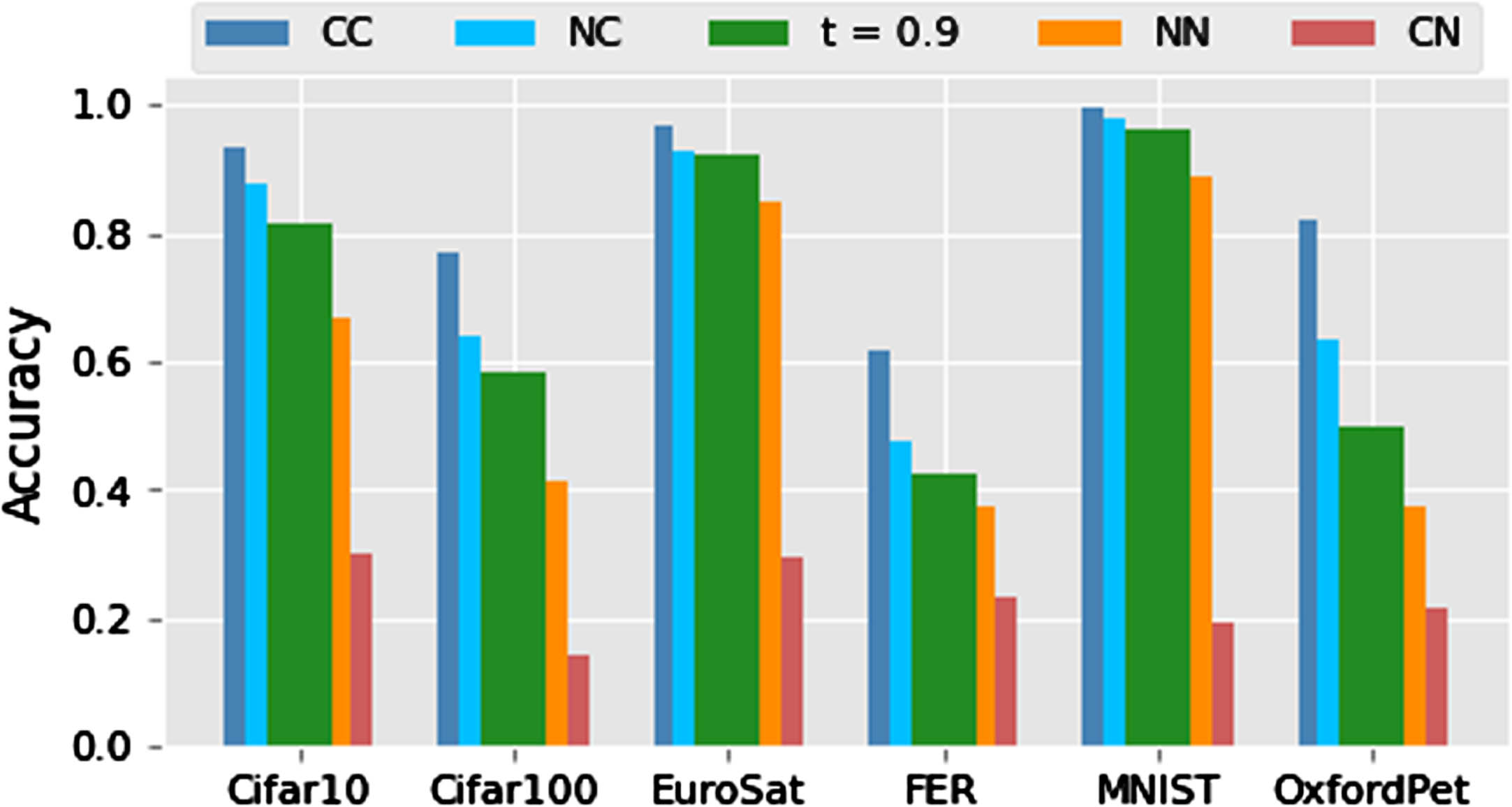
The average accuracy of the object classifier predictions achieved by our approach (with a confidence threshold t = 0.9) w.r.t. the baselines is shown in Fig. 5. Our approach achieves good accuracy in all domains when compared to the NC version, i.e., the agent computes and executes plans that effectively lead to belief states where the perception function for the object types is more reliable. Our method achieves good accuracy relative to version NC in all domains, i.e., the agent produces and executes plans to effectively reach belief states where the perception function for the object types is more accurate. The overall performance of our method decreases in domain FER, where the classification task is more complex since CC achieves the worst performance. Our method outperform the performance of the NN baseline significantly (i.e. at least 10%) in all domains but FER. This improvement is an empirical evidence of the importance of planning and acting to reach states where the agent can better observe a state variable. Finally, baseline CN achieves the worst accuracy, which is significantly lower than NN accuracy. This is due to the fact that the perception function for CN is trained in fully observable environments and tested in partially observable environments.

Fig. 5

Accuracy of the object type predictions for each dataset.

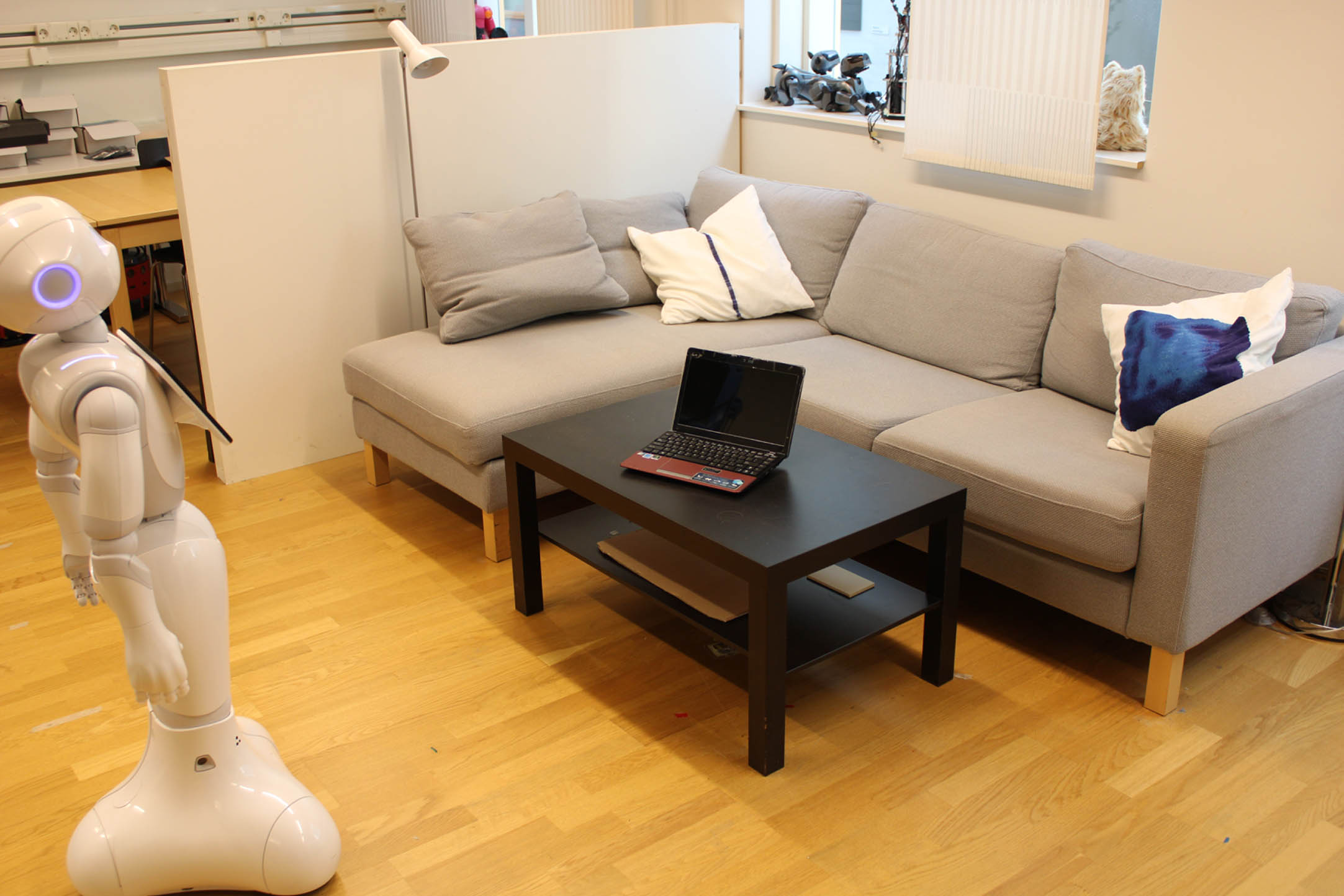
7.3 Real world experiments

To show the feasibility of our approach in a real-world environment, we experiment with a Softbank Robotic’s Pepper humanoid robot with noisy sensors (e.g., RGB and depth camera) and actuators in PEIS home ecology [37], shown in Fig. 6. Pepper moves in a living room where there is a table with some objects on top of it (e.g., a mug, a laptop). The task consists of perceiving an object property that is observable. For instance, the property filled for objects of type mug can be observed only when looking at the top of the mug. For every object property to be learned, Pepper firstly collects online a number of observations (set to 200 in our experiments), according to Algorithm 1, and trains a neural network for recognizing the property. For example, Pepper asks a human to fill the mug, takes a number of images of the filled mug, and labels them with the action effect specified in a symbolic (PDDL) domain. The control variables associated with each observation are the distance, yaw angle, and pitch angle between Pepper camera and the object. The control variable values are computed by Pepper’s noisy depth image, and noisy odometry position. By applying Algorithm 2, Pepper evaluates the confidence of the neural network on the acquired observations, and clusters the observations according to the control variable values and the neural network confidence.

Fig. 6

Pepper taking images of a laptop and asking a human to manipulate it for learning the property on.

For clustering, we adopted the K-means algorithm with K = 8. The viewpoints where the property is observable consists of the clusters with an average confidence higher than a threshold t = 0.8.

In Table 4, we evaluate the determined viewpoints by means of their precision and recall w.r.t. the observability of a number of properties of different objects. For this evaluation, we manually labeled the observations acquired by Pepper as observable and not observable. Hence, true positives are observations in the determined viewpoints where the property can be actually observed; whereas false positives consists of observations in the determined viewpoints where the property cannot be observed. Similarly, observations that do not belong to any viewpoint are true negatives when the property is not observable and false negatives when the property is observable. The results in Table 4 empirically show that our method can effectively find viewpoints where properties are better observable. For all object types but laptop, the determined viewpoints are composed of observations where the property is always observable (i.e., the precision equals 1). However, for object types big/small bowl and chair, the recall is low, i.e., the agent does not find all viewpoints where properties can be observed.

Table 4

Precision and recall of the viewpoints w.r.t. the observability of a number of properties of different objects

Object type	Property	Precision	Recall
cup	filled	1	0.66
mug	filled	1	0.94
laptop	on	0.61	0.98
big bowl	full	1	0.18
small bowl	full	1	0.31
chair	free	1	0.28
Average	-	0.94	0.56

We also evaluate the ability of Pepper to plan and act for getting into a determined viewpoint and better observing the object properties. To this aim, Pepper starts in a random position, and is asked to predict some object properties. Firstly, Pepper observes the object and checks whether its current state belongs to a previously learned viewpoint, possibly planning and acting for reaching a viewpoint. Finally, Pepper predicts the truth value of the property. The above process is repeated 20 times for each object property. We compare our approach with baseline NN, which assumes that the property can be always observed and hence does not plan to reach a viewpoint before predicting the property. The accuracy of the predictions achieved by our method compared to baseline NN is reported in Fig. 7. More precisely, we show the accuracy of property predictors trained for a varying number of epochs. The results show that planning and acting for reaching the learned viewpoints allows Pepper to improve its ability of correctly predicting the truth value of the object properties.

Fig. 7

Accuracy of the predictions of the object properties averaged over all properties and objects reported in Table 4. The width of the colored areas measures the standard deviation of the accuracy.

8 Conclusions and future work

We propose a general architecture integrating planning, learning and acting, and we address the challenge of using symbolic planning to automate the learning of perception capabilities. Moreover, we extend the proposed method to learn the situations where a state variable is observable, and reach such situations by planning and acting.

We experimentally show that our approach is feasible and effective for recognizing object types in a number of synthetic datasets, and object properties in both simulated and real-world environments involving noisy perceptions and noisy actions on a real robot.

Still a lot of work must be done to address the general problem of planning and acting to learn in a physical environment. For example, planning for online training the object detector from a few examples or learning relations among different objects. We assume that the agent can always change the truth value of the observable variables, eventually asking for the help of a human. In future work, we will investigate how the agent can change such value without knowing it.

Footnotes

Acknowledgments

We thank Luciano Serafini, Paolo Traverso, Alfonso Gerevini and Alessandro Saetti for their help and supervision of previous work on the integration of planning, learning and acting. We acknowledge the support of the PNRR project FAIR - Future AI Research (PE00000013), under the NRRP MUR program funded by the NextGenerationEU. This work has also been partially supported by TAILOR project funded by the EU Horizon 2020 research and innovation program under GA n. 952215.

Quotes indicate names for elements of $P$ .

References

Aineto

, Jiménez

, Onaindia

, Learning action models with minimal observability, Journal of Artificial Intelligence (AIJ) 275 (2019), 104–137.

Masataro

Asai , Unsupervised grounding of plannable firstorder logic representation from images. In ICAPS, 2019.

Masataro

Asai and

Alex

Fukunaga , Classical planning in deep latent space: Bridging the subsymbolic-symbolic boundary. In AAAI, 2018.

Christer

Bäckström and

Bernhard

Nebel , Complexity results for sas+ planning, Computational Intelligence 11(4) (1995), 625–655.

Jeannette

Bohg ,

Karol

Hausman ,

Bharath

Sankaran ,

Oliver

Brock ,

Danica

Kragic ,

Stefan

Schaal and

Gaurav

Sukhatme , Interactive perception: Leveraging action in perception and perception in action, IEEE Transactions on Robotics 33 (2017), 1273–1291.

Blai

Bonet and

Hector

Geffner , Learning first-order symbolic representations for planning from the structure of the state space. In ECAI, 2020.

Tommaso

Campari ,

Leonardo

Lamanna ,

Paolo

Traverso ,

Luciano

Serafini , and

Lamberto

Ballan , Online learning of reusable abstract models for object goal navigation. In Proceedings of the IEEE/CVF Conference on Computer Vision and Pattern Recognition, pages 14870–14879, 2022.

Silvia

Coradeschi and

Alessandro

Saffiotti , An introduction to the anchoring problem, Robotics and Autonomous Systems 43(2–3) (2003), 85–96.

Stephen

Cresswell ,

Thomas Leo

McCluskey and

Margaret Mary

West , Acquiring planning domain models using LOCM, Knowledge Eng. Review 28(2) (2013), 195–213.

10.

Nils

Dengler ,

Tobias

Zaenker ,

Francesco

Verdoja and

Maren

Bennewitz , Online object-oriented semantic mapping and map updating. In 2021 European Conference on Mobile Robots (ECMR), pages 1–7. IEEE, 2021.

11.

Manfred

Eppe ,

P.D.

Nguyen and

Stefan

Wermter , From semantics to execution: Integrating action planning with reinforcement learning for robotic tool use. arXiv preprint arXiv:1905.09683, 2019.

12.

Kutluhan

Erol ,

James A.

Hendler and

Dana S.

Nau , Umcp: A sound and complete procedure for hierarchical task-network planning. In Proceedings of the 2nd International Conference on Artificial Intelligence Planning Systems, pages 249–254, 1994.

13.

Glenn Jocher et al. ultralytics/yolov5: v6.0 - YOLOv5n ‘Nano’ models, Roboflow integration, TensorFlow export, OpenCV DNN support, October, 2021.

14.

Ghallab ,

D.S.

Nau ,

Traverso , Automated Planning and Acting. Cambridge University Press, 2016.

15.

Maxence

Grand ,

Damien

Pellier and

Humbert

Fiorino , Amlsi: A novel accurate action model learning algorithm. In International Workshop on Knowledge Engineering for Planning and Scheduling (KEPS) during the 30th International Conference on Automated Planning and Scheduling (ICAPS, 2020), 2020.

16.

Peter

Gregory and

Stephen

Cresswell , Domain model acquisition in the presence of static relations in the lop system. In Proceedings of the International Conference on Automated Planning and Scheduling 25 (2015), 97–105.

17.

Kaiming

He ,

Xiangyu

Zhang ,

Shaoqing

Ren and

Jian

Sun , Deep residual learning for image recognition. In Proceedings of the IEEE Conference on Computer Vision and Pattern Recognition, pages 770–778, 2016.

18.

Malte

Helmert

, The fast downward planning system, Journal of Artificial Intelligence Research 26 (2006), 191–246.

19.

Michael

Janner ,

Sergey

Levine ,

William T.

Freeman ,

Joshua B.

Tenenbaum ,

Chelsea

Finn and

Jiajun

Wu , Reasoning about physical interactions with object-oriented prediction and planning, arXiv preprint arXiv:1812.10972 2018.

20.

Brendan

Juba ,

Hai S.

Le and

Roni

Stern , Safe learning of lifted action models. In

Meghyn

Bienvenu ,

Gerhard

Lakemeyer , and

Esra

Erdem , editors, Proceedings of the 18th International Conference on Principles of Knowledge Representation and Reasoning, KR 2021, Online event, November 3-12, 2021, pages 379–389, 2021.

21.

Eric

Kolve ,

Roozbeh

Mottaghi ,

Winson

Han ,

Eli

VanderBilt ,

Luca

Weihs ,

Alvaro

Herrasti ,

Daniel

Gordon ,

Yuke

Zhu ,

Abhinav

Gupta and

Ali

Farhadi , AI2-THOR: An Interactive 3D Environment for Visual AI. arXiv, 2017.

22.

George

Konidaris ,

Leslie Pack

Kaelbling and

Tomás

Lozano- Pérez , From skills to symbols: Learning symbolic representations for abstract high-level planning. J. Artif. Intell. Res., 61: 215–289, 2018.

23.

George

Konidaris ,

Leslie Pack

Kaelbling and

Tomas

Lozano-Perez , From skills to symbols: Learning symbolic representations for abstract high-level planning. Journal of Artificial Intelligence Research 61:215–289, 2018.

24.

Leonardo

Lamanna ,

Alfonso Emilio

Gerevini ,

Alessandro

Saetti ,

Luciano

Serafini and

Paolo

Traverso , On-line learning of planning domains from sensor data in pal: Scaling up to large state spaces. In Proceedings of the AAAI Conference on Artificial Intelligence, 35 (2021), 11862–11869.

25.

Leonardo

Lamanna ,

Alessandro

Saetti ,

Luciano

Serafini ,

Alfonso

Gerevini and

Paolo

Traverso , Online learning of action models for pddl planning. In IJCAI-2021, 2021.

26.

Leonardo

Lamanna ,

Luciano

Serafini ,

Alessandro

Saetti ,

Alfonso Emilio

Gerevini and

Paolo

Traverso , Online grounding of symbolic planning domains in unknown environments. In Proceeding of the 19th International Conference on Principles of Knowledge Representation and Reasoning, KR (2022), 2022.

27.

Leonardo

Lamanna ,

Luciano

Serafini ,

Mohamadreza

Faridghasemnia ,

Alessandro

Saffiotti ,

Alessandro

Saetti ,

Alfonso

Gerevini and

Paolo

Traverso , Planning for learning object properties. In Proceedings of the AAAI Conference on Artificial Intelligence, 2023. doi: 10.48550/ARXIV.2301.06054.

28.

Andrés Occhipinti

Liberman ,

Blai

Bonet and

Hector

Geffner , Learning first-order symbolic planning representations that are grounded, CoRR, abs/2204.11902, 2022.

29.

Thomas Leo

McCluskey ,

Stephen

Cresswell ,

Elisabeth Richardson and

Margaret

Mary West , Automated acquisition of action knowledge. In ICAART, 2009.

30.

Toki

Migimatsu and

Jeannette

Bohg , Grounding predicates through actions. In 2022 International Conference on Robotics and Automation (ICRA), pages 3498–3504. IEEE, 2022.

31.

Mnih

, Kavukcuoglu

, Silver

, Rusu

A.I.A.

, Veness

, Bellemare

M.G.

, Graves

, Riedmiller

M.A.

, Fidjeland

, Ostrovski

, Petersen

, Beattie

, Sadik

, Antonoglou

, King

, Kumaran

, Wierstra

, Legg

and Hassabis

, Human-level control through deep reinforcement learning, Nature 518(7540) (2015), 529–533.

32.

Volodymyr

Mnih ,

Adria Puigdomenech

Badia ,

Mehdi

Mirza ,

Alex

Graves ,

Timothy

Lillicrap ,

Tim

Harley ,

David

Silver and

Koray

Kavukcuoglu , Asynchronous methods for deep reinforcement learning. In International conference on machine learning, pages 1928–1937 PMLR, 2016.

33.

Natale

, Metta

and Sandini

, Learning haptic representation of objects. In International Conference on Intelligent Manipulation and Grasping 2004.

34.

Adam

Paszke ,

Sam

Gross ,

Francisco

Massa ,

Adam

Lerer ,

James

Bradbury ,

Gregory

Chanan ,

Trevor

Killeen ,

Zeming

Lin ,

Natalia

Gimelshein ,

Luca

Antiga , et al. Pytorch: An imperative style, high-performance deep learning library, Advances in Neural Information Processing Systems 32 (2019), 8026–8037.

35.

Lerrel

Pinto ,

Dhiraj

Gandhi ,

Yuanfeng

Han ,

Yong-Lae

Park and

Abhinav

Gupta , The curious robot: Learning visual representations via physical interactions. In European Conference on Computer Vision (ECCV), pages 3–18. Springer, 2016.

36.

Stuart J.

Russell and

Peter

Norvig , Artificial intelligence a modern approach, Pearson Education, Inc, 2010.

37.

Alessandro

Saffiotti ,

Mathias

Broxvall ,

Marco

Gritti ,

Kevin

LeBlanc ,

Robert

Lundh ,

Jayedur

Rashid ,

Beom-Su

Seo and

Young-Jo

Cho , The peis-ecology project: Vision and results. In 2008 IEEE/RSJ International Conference on Intelligent Robots and Systems, pages 2329–2335, 2008. doi: 10.1109/IROS.2008.4650962.

38.

Gabriele

Sartor ,

Angelo

Oddi ,

Riccardo

Rasconi and

Vieri Giuliano

Santucci , Intrinsically motivated high-level planning for agent exploration. In International Conference of the Italian Association for Artificial Intelligence, pages 119–133. Springer, 2023.

39.

Sutton

R.S.

, Barto

A.G.

Reinforcement learning – an introduction, Adaptive Computation and Machine Learning. MIT Press, 1998.

40.

Emre

Ugur and

Justus

Piater , Bottom-up learning of object categories, action effects and logical rules: From continuous manipulative exploration to symbolic planning. In International Conference on Robotics and Automation (ICRA), pages 2627–2633. IEEE, 2015.