A new perspective on optimizers: leveraging moreau-yosida approximation in gradient-based learning

1 Introduction

Gradient-based optimization is undeniably a cornerstone of Machine Learning (ML), with deep learning’s remarkable success heavily reliant on the efficiency of Stochastic Gradient Descent (SGD) for solving large-scale optimization problems [3]. The conventional approach to describe gradient descent-based optimization in Euclidean spaces, make use of its geometrical interpretation of direction of steepest descent [5]. This interpretation gives rise to the definition of gradient descent as an iterative procedure. Specifically, given a loss function ℒ to be minimized, which depends on parameters w ∈ ℝ N , the update scheme at the k-th step of gradient descent, denoted by w ^k , is expressed as: w k + 1 = w k - τ ∇ ℒ ( w k ) ,(1) where, for some initial w⁰ = w₀ ∈ ℝ ^N , τ > 0 serves as the learning rate or step size and ∇ℒ represents the gradient of ℒ with respect to w.

The Machine Learning (ML) literature contains numerous works that propose adaptive values for τ, customized learning rates for individual components of w, or additional terms in the update rules [7, 24]. However, these approaches are based on different principles and presented from diverse problem formulations, making it challenging to compare them directly. Simply examining the final update rules is insufficient to fully grasp the expected effects they bring to optimization. While tracing connections among these methods is possible, it is not straightforward.

To address this issue, we propose a unified view that recasts these update rules into a coherent framework. In this view, w^k+1 is treated as the solution of a newly introduced optimization problem with well-defined and interpretable regularity conditions. These conditions govern the variation between w ^k and w^k+1, making it easier to understand the properties of the solution (w^k+1) and to compare different approaches. Our inspiration lies in the Moreau-Yosida (MY) approximation of a function [1], which we apply to the loss function ℒ. Notably, we find analogies between the stationary condition defining the MY approximation and the update rules in the form of Equation (1). However, directly dealing with this approximation is insufficient to recover the update scheme of Equation (1). Hence, we investigate the first-order Taylor expansion of ℒ in the MY approximation, leading us to devise a related optimization problem whose solution is equivalent to Equation (1) under certain regularity conditions. Beyond enhancing interpretability, our primary goal is to provide researchers with a formulation that facilitates the development of novel, more informed optimizers. Although a related approach exists in the online learning community [4], it remains relatively unknown to the wider ML audience. Our approach in not concerned with the specific studies of regularization or implicit regularization properties of SGD [19, 26] but instead is about a general framework to describe several optimization methods used in ML literature.

To demonstrate the practical utility of our unified view, in Section 4, we investigate a case-study involving the MY approximation to design a novel update scheme for neural network weights. This scheme modulates the update strength according to the variations of the predictions over time. Strong output variations indicate significant changes in the data, requiring the network to be more adaptable to novel information. In contrast, small variations trigger less substantial updates, preserving learned information and promoting stability. We experimentally explore this criterion in an online learning problem [6, 18], where data is continuously provided. We showcase how this regularization principle, typically used in Manifold Regularization [2, 16], can be directly injected into the update rule of model parameters for continual learning. We also present results obtained in an offline-learning setting.

OPEN IN VIEWER

Fig. 1

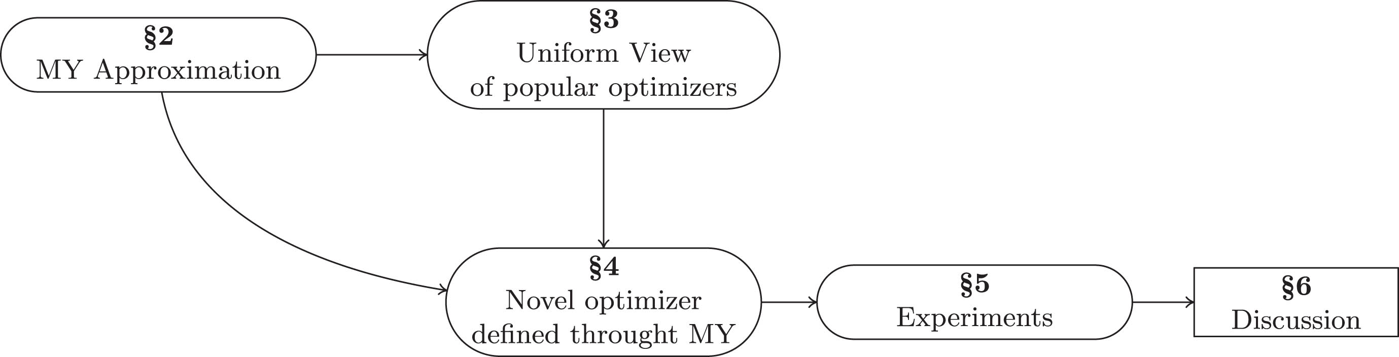
Conceptual scheme of the organization of the article, that highlights the main theoretical contributions.

In this section, we formally introduce the Moreau-Yosida (MY) approximation, defined as Def. 2.1, which serves as the foundation for our approach. Subsequently, we leverage this notion to establish an update scheme, Equation (8), based on an optimization problem whose minima correspond to the solution of the recursive rule found in gradient-based methods. The MY approximation is a well known tool mainly used in convex analysis and it belongs to a class of more general operations called infimal convolutions [22].

Definition 2.1. (MY Approximation) Given a nonnegative, lower semicontinuous function ℒ: ℝ ^N  → ℝ, commonly encountered in implementations of the empirical risk in Machine Learning, the Moreau-Yosida approximation [1] of ℒ evaluated at point w, denoted as ℒ_MY (w), is defined as follows: 1 . ℒ MY ( w ) : = min w ′ ∈ ℝ N ℒ ( w ′ ) + 1 2 τ ∥ w ′ - w ∥ 2 ,(2) where ∥· ∥ is the Euclidean norm and τ > 0.

OPEN IN VIEWER

Fig. 2

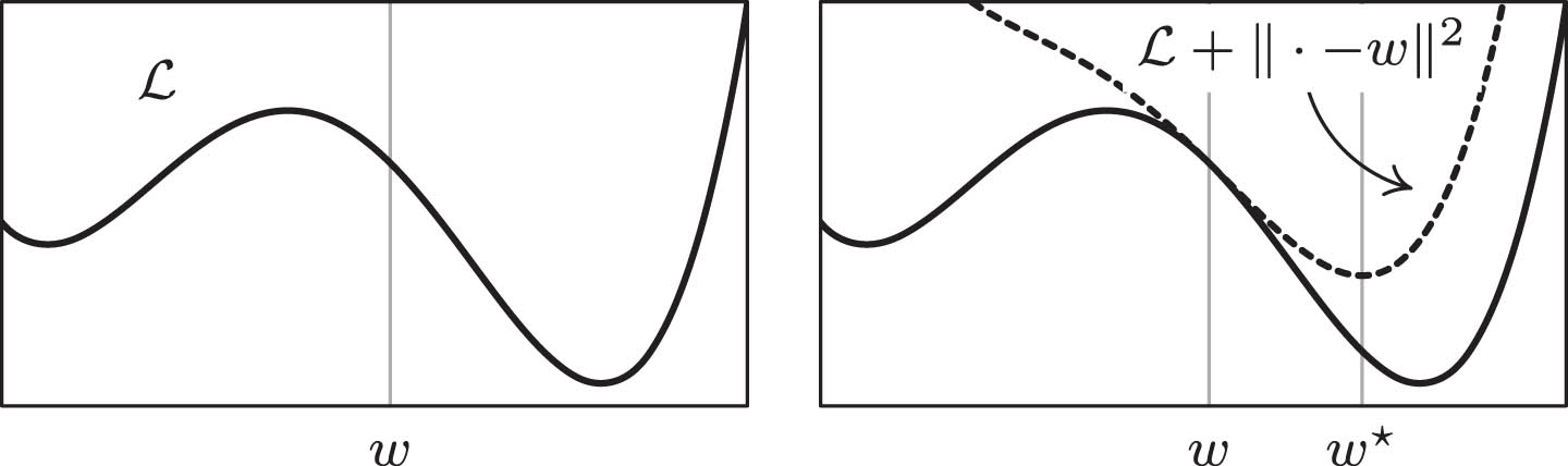
MY approximation for ℒ (w) = (w^′2 - 4/5) ² - w^′/4 at the point w = 1/4. The dotted line represents the function ℒ (w^′) + (w^′ - w) ²/(2τ) with the choice τ = 1/2. According to Equation (4) the step w → w^★ can be interpreted as an implicit GD step on the function ℒ.

The optimization problem in Equation (2) consists of an objective function composed of two terms. The left-most term represents the value of ℒ evaluated at w^′, which typically denotes a loss function aggregated over the available data. Here, w^′ serves as the variable to be minimized. On the other hand, the right-most term serves as a regularizer, penalizing significant variations between w^′ and the target point of the approximation, w. As a result, given w^★ that minimizes the objective function of Equation (2) w ★ ∈ arg min w ′ ∈ ℝ N ℒ ( w ′ ) + 1 2 τ ∥ w - w′ ∥ 2 ,(3) we can express the Moreau-Yosida (MY) approximation of ℒ evaluated at w as: ℒ MY ( w ) = ℒ ( w ★ ) + 1 2 τ ∥ w ★ - w ∥ 2 .(4) Here, a smaller value of τ enforces w^★ and w to be closer in the sense of standard Euclidean topology. In the context of hard-constrained optimization, the problem in Equation (2) is conceptually equivalent to the following constrained optimization problem: min w ′ ∈ ℝ N ℒ ( w ′ ) ; s . t . ∥ w - w′ ∥ ≤ ε , where ε > 0 decreases as τ decreases. This highlights the spatial locality of the MY approximation. Clearly, when we are considering continuos loss functions, the stationary points of Equation (2) are those w^★ for which the gradient ∇ℒ of ℒ is null, 2 , thus ∇ℒ (w^★) + (w^★ - w)/τ = 0, which requires: w ★ = w - τ ∇ ℒ ( w ★ ) ,(5) which is a different way to represent Equation (3).

Recovering Gradient-based Learning. Let us examine the sequence of points (^wk) _k≥0 following the classic recursive rule of gradient-based methods with learning rate τ, Equation (1), { w 0 = w 0 ∈ ℝ N ; w k + 1 = w k - τ ∇ ℒ ( w k ) , k > 0 .(6) where w₀ is a given starting point. We can leverage the MY approximation of ℒ in Equation (2) and, specifically, the expression of the argument minimizing the MY approximation (Equation (3)), to derive a related recursive relation. By replacing w^★ with w^k +1 and w with w ^k , we obtain 3 : w k + 1 ∈ arg min w ′ ∈ ℝ N ℒ ( w ′ ) + 1 2 τ ‖ w ′ - w k ‖ 2 , k > 0 .(7) This equation, in accordance with Equation (4), is equivalent to the following scheme: w k + 1 = w k - τ ∇ ℒ ( w k + 1 ) , k > 0 .(8) It is evident that Equation (7) describes an implicit scheme, where w^k +1 cannot be directly computed, as it appears on both sides of the equation. This is distinct from Equation (5), which represents an explicit scheme. For practical applications in machine learning, it is crucial to rely on explicit schemes since solving the implicit Equation (6) is often unfeasible. To recover the explicit gradient descent method from the MY approximation, we can make a further step. Whenever ℒ is smooth, at least in the neighborhoods of w ^k , we can approximate the value of ℒ using a first-order truncated Taylor expansion: ℒ ( w ′ ) ≈ ℒ ( w k ) + ∇ ℒ ( w k ) · ( w ′ - w k ) , where · denotes the standard scalar product in ℝ ^N . By applying this approximation in Equation (6) and dropping the constant term ℒ (w ^k ) since it does not affect the optimization problem, we obtain for k > 0: w k + 1 ∈ arg min w ′ ∈ ℝ N ∇ ℒ ( w k ) · ( w ′ - w k ) + 1 2 τ ‖ w ′ - w k ‖ 2 .(9) Solving Equation (8) for w′ = w^k +1 leads us to the equation of the stationary points ∇ℒ (w ^k ) + (w^k +1 - w ^k )/τ = 0. Ultimately, this yields w^k +1 = w ^k  - τ ∇ ℒ (w ^k ), which is precisely the explicit gradient descent method of Equation (5).

Thus, Equation (8) represents the MY-based view of gradient-based methods, equivalent to the explicit gradient descent scheme.

Uniform View. The MY scheme presented in Equation (8) offers a clear understanding of the role played by the variation between w^′ = w^k +1 and w ^k , which influences both the squared regularizer (weighted by the learning rate τ) and the modulating term of the gradient of the loss function ℒ. This formulation serves as a powerful and versatile tool capable of describing various variants of gradient-based updates, commonly known as optimizers. By adjusting either the regularizer ||w^′ - w ^k ||² or adapting ∇ℒ, we can readily discern the expected properties of the resulting update rule of many commonly used optimizer. We will explore this topic in the subsequent Section 3. In contrast, Section 4 discuss a case-study where we introduce a novel gradient-based method, exemplifying the versatility of this unified view in designing innovative optimizers.

In this section, we will discuss how the MY view of Equation (8) is general enough to can describe several existing optimizers widely employed in the ML community. In particular, we will consider the case of Stochastic Gradient Descent (SGD) [21], Heavy Ball method (gradient descent with momentum) [20], AdaGrad [7], RMSprop [24], and ADAM [11].

SGD. Equation (8) We begin with the widely recognized Stochastic Gradient Descent method [21], a technique rooted in a stochastic objective that engages a fraction of the available data during each iteration. This example serves as a pretty straightforward case to cast in the MY view, but also as our initial reference point for introducing additional notation. Our context involves a training set comprising n samples, with the loss function expressed as ℒ = ( 1 / n ) ∑ i = 1 n ℒ i , where _ℒi signifies the loss computed for the i-th instance. During each iteration of the gradient descent process, a mini-batch is drawn, constituting a set of independently (and randomly) selected data. Denoting the set of m indices belonging to the k-th mini-batch as I _k , and the loss function evaluated on this mini-batch as (1/m) ∑_{i∈I k ℒi} (w ^k ), the standard SGD update is w k + 1 = w k - τ 1 m ∑ i ∈ I k ∇ ℒ i ( w k ) , k > 0 . The MY perspective naturally emerges without altering the squared regularization term, as expected. A straightforward transition involves substituting ∇ℒ (w ^k ) in Equation (5) with (1/m) ∑_{i∈I k}  ∇ _ℒi (w ^k ), yielding the following expression: w k + 1 ∈ arg min w ′ ∈ ℝ N g k · ( w ′ - w k ) + 1 2 τ ‖ w ′ - w k ‖ 2 ,(11) for k > 0, where g _k  : = (1/m) ∑_{i∈I k}  ∇ ℒ _i  (w ^k ), which we will maintain throughout the paper for its versatility in reverting to classic full-batch gradient descent when g _k is set to ∇ℒ (w ^k ).

Heavy Ball Method. Also recognized as gradient descent with momentum [20], the Heavy Ball method employs an explicit formula that incorporates the most recent parameter variation, w ^k  - w^k - 1, as follows: w k + 1 = w k - α g k + β ( w k - w k - 1 ) , k > 0 ,(12) where α and β are positive constants. The MY perspective can be achieved by introducing a higher-order regularization term and expressing α and β as α = μτ/(μ + τ) and β = τ/(μ + τ), resulting in the form: w k + 1 ∈ arg min w ′ ∈ ℝ N g k · ( w ′ - w k ) + ‖ w ′ - w k ‖ 2 2 τ + ‖ w ′ - 2 w k + w k - 1 ‖ 2 2 μ ,(13) for k > 0. Notably, the MY view underscores that, compared to standard gradient descent, the Heavy Ball method introduces an additional regularization term (weighted by 1/(2μ)) that enforces second-order information into the update step. More explicitly, in gradient descent with momentum the update step is designed not only in such a way that the values of the weights are not too far away but also trying to avoid abrupt variations in the “way” weights change; a sort of regularization on the velocity of the weights. An alternative rendition of this method is sometimes provided using exponential averages, which can also be framed within the MY view. Given a sequence (a _k ) _k≥0, the exponential moving average with discount factor δ is represented as ( 〈 a 〉 k δ ) k ≥ 0 , where the k-th term is computed as: 〈 a 〉 k δ : = ( 1 - δ ) ∑ j = 0 k δ k - j a j .(14)

Using this concept, an alternative form of the update rule in Equation (11) can be expressed as w k + 1 = w k - τ 〈 g 〉 k β . In this case, the MY view can be reformulated as: w k + 1 ∈ arg min y ∈ ℝ N 〈 g 〉 k β · ( y - w k ) + 1 2 τ ‖ y - w k ‖ 2 ,(15) for k > 0, which involves replacing the gradient term g _k with its exponential moving average with decay factor β. This version substitutes higher-order regularity with a smoothing operation on the gradient term g _k . We will also use this alternative form when discussing the ADAM algorithm.

AdaGrad and RMSprop. Both techniques (discussed in [7] and [24]) can be aligned with the MY view in a similar manner. Their update schemes are defined as w k + 1 = w k - τ ( H k ) - 1 g k , k > 0 . Here, H _k is a diagonal matrix with specific diagonal elements: ( H k ) ii : = { + ∑ n = 0 k ( g i n ) 2 ; for AdaGrad + ∑ n = 0 k 〈 g i 2 〉 n β , for RMSprop , where ε > 0, i ∈ {1, 2, …, N}, g i k is the i-th component of the gradient, and ( g i 2 ) n : = ( g i n ) 2 is the sequence of squared gradient components for fixed i. Incorporating the MY view involves changing the metric used to assess the proximity of the next point to the current w ^k . Specifically, both methods stem from Equation (10) through the substitution ||w′ - w ^k ||²/(2τ) ⟶ (w′ - w′ ^k ) · H _k  (w′ - w ^k )/(2τ). This substitution underlines the shift in metric due to matrix H _k when evaluating the regularization term in parameter variation. In this way, in each direction the penalty of the closeness of the next step can be suitably modulated and differentiated.

ADAM. As a well-known optimization method, ADAM [11] combines gradient descent with momentum and RMSprop in a specific way. To express ADAM within the Moreau-Yosida regularization framework, we first need to introduce a further concept: the normalized exponential moving average. Let ( 〈 a 〉 k γ ) k ≥ 0 denote the exponential moving average of the sequence (a _k ) _k≥0 with discount factor δ. We define the normalized exponential moving average as 〈 a 〉 ˆ k δ : = 〈 a 〉 k δ 1 - δ k + 1 , k ≥ 0 .(16) The ADAM update scheme becomes w k + 1 = w k - τ ( H ˆ k ) - 1 〈 g 〉 ˆ k β 1 , k > 0 , where H ˆ k is a diagonal matrix with ( H ˆ k ) ii = ε + ∑ n = 0 k 〈 g i 2 〉 ˆ n β 2 , i ∈ { 1 , … , N } , and β₁ and β₂ are customizable parameters of the ADAM algorithm. Applying a procedure similar to what we did for the Heavy Ball method, using Equation (15), we can express ADAM in the context of the Moreau-Yosida view as w k + 1 ∈ argmin y ∈ ℝ N 〈 g 〉 ˆ k β 1 · ( y - w k ) + 1 2 τ ( y - w k ) · H ˆ k ( y - w k ) ,(17) for k > 0. In this representation, it is noticeable (i) the metric change in the regularity term due to matrix H ˆ k , and (ii) the smoothing operation on g _k , which, as discussed in the case of the Heavy Ball method, indirectly introduces a higher-order regularity condition on the weight variation. Notice that the classic ADAM scheme here has been derived putting together the quadratic regularization term induced by the matrix H _k of RMSprop and the formulation of gradient descent with momentum based on(). However the adoption of the MY view makes it clear that RMSprop and momentum could have been put together also by using the form for the momentum described in Equation (12), yielding a variant of the ADAM method that would have been extremely difficult to individuate with the classical formulation of the optimization method.

When introducing the MY view of Section 2, we discussed essentially how a gradient step is equivalent to solving a local minimization problem on a risk ℒ around the current step w ^k . As a proof-of-concept of the versatility of this view toward the design of novel optimizers, we consider a specific use-case based on neural networks.

Continual Learning, Non-i.i.d. data. Consider a neural network net (· , w) : ℝ ^d  → ℝ ^p with weights w ∈ ℝ ^N , mapping input data x ∈ ℝ ^d to output net (x, w) ∈ ℝ ^p . The network’s performance is quantified by the risk ℒ. We delve into the realm of continual learning, where data samples lack the independence and identical distribution (i.i.d.) assumption. This scenario arises due to sequential presentation of tasks and related data, leading to evolving data distributions over time [8, 18]. Consequently, learning encounters sequences of similar or related samples and abrupt shifts between tasks. The model’s plasticity must adapt accordingly, being more receptive to novel, unseen data while avoiding overfitting of frequently observed recent data. We conjecture that variations in network outputs might indirectly signal data similarity or task transitions. It is essential to emphasize that we are not aiming to address catastrophic forgetting or propose a novel continual learning algorithm. Instead, our focus is on presenting a case study that illustrates the ease of incorporating new knowledge into the update process using the MY view.

Output-based Modulation. In Equation (6), parameter closeness relies on ||w′ - w ^k ||²/(2τ). Our aim is to enhance this Euclidean topology by accounting for how parameter changes, induced by learning, and their interaction with variations in model outputs. To achieve this, we introduce a modulation function ψ (ν) that leverages network outputs ν to adjust the regularization term in Equation (6). This prompts us to explore gradient descent variations achieved by transforming the “distance” term as follows: 1 2 τ ‖ w ′ - w k ‖ 2 ⟶ ψ ( ν ) 2 τ ‖ w ′ - w k ‖ 2 .(18) The MY view, by explicitly revealing the regularizer governing weight variations, enables us to immediately connect the modulated term with its implications for the update rule. We delve into this connection by detailing the structure of ψ (ν) and its impact on the update procedures. Since network outputs depend on input data and parameter values, it is crucial to define a consistent protocol for introducing data to the learning process.

Choosing the Modulation Function ψ. At each time step, we are provided with a mini-batch of data containing m samples, indexed as previously defined by I _k . Building on the definition of g _k as seen in the SGD case, where g k = 1 m ∑ i ∈ I k ∇ f i ( w k ) , we unveil our proposal for the modulation function ψ: ψ ( ν ) : = m 2 γ k ‖ ∑ i ∈ I k ν ( x i , w k ) - ∑ j ∈ I k - 1 ν ( x j , w k - 1 ) ‖ - 2 ,(19) Here, γ _k  > 0 acts as a normalization factor, potentially varying over time (denoted by the subscript). When the network’s average outputs between step k - 1 and k are akin, ψ (ν) diminishes, and conversely. This choice of ψ (ν) connects the modulation strength to the similarity of the network’s past and present outputs.

We now proceed to frame the MY view incorporating output modulation. The updated formulation becomes: w k + 1 ∈ arg min w ′ ∈ ℝ N g k · ( w ′ - w k ) + 1 2 τ m 2 ‖ w ′ - w k ‖ 2 γ k ‖ ∑ i ∈ I k ν ( x i , w k ) - ∑ j ∈ I k - 1 ν ( x j , w k - 1 ) ‖ 2(20) for k > 0. By computing the stationarity condition of the objective function, we deduce the iterative update rule: w k + 1 = w k - τ γ k ‖ 1 m ∑ i ∈ I k ν ( x i , w k ) - 1 m ∑ j ∈ I k - 1 ν ( x j , w k - 1 ) ‖ 2 g k , for k > 0. Our forthcoming section will delve into empirical exploration of this proposed method encapsulated by Equation (19), enabling us to investigate the effectiveness of our regularization approach.

We proceed to assess the impact of the introduced regularization term, as detailed in Section 4. To this end, we set up two classes of experiments. In the first class, we used the widely recognized MNIST dataset to conduct three experiments termed Permuted MNIST, Non i.i.d. MNIST, and MNIST. In the second class, we devised a more challenging scenario using both the MNIST and CIFAR-10 datasets, which we denote as Progressive Permuted MNIST and Progressive Permuted CIFAR-10. Importantly, it should be noted that our aim is to empirically gauge the effects of the proposed optimizers within the framework of our case study. We do not intend to present an approach that directly rivals the current state-of-the-art methodologies since it is clear that specific continual learning techniques will in general outperform our generic output-based modulation approach. We report the main features of each experiment in the following list.

1. Permuted MNIST: This experiment serves as a benchmark for continual learning on MNIST data, where the data distribution remains non-stationary.

2. Non i.i.d. MNIST: This experiment dives into situations with highly temporally dependent data samples.

3. MNIST: This scenario deviates from the aforementioned case-study setups and is a classic MNIST experiment. It involves training the network ν in an offline manner. This allows us to study how the output regularization term behaves in a standard benchmark, comparing its impact on performance against a vanilla gradient method.

4. Progressive Permuted MNIST/CIFAR-10: Here, we explore the effects of output regularization in scenarios with gradual shifts in data distribution, ensuring a temporal consistency in the evolving tasks.

In all these experiments, we set the normalization term γ _k of Equation (19) as γ _k  = ||∑_{i∈I k} ν (x _i , w ^k )/m||^-2 to enable relative comparisons between outputs at various time steps. Additionally, in all experiments, the ADAM optimizer replaces standard SGD for quicker convergence. The learning rate parameter τ in Equation (16) is used. For the MNIST experiments we considered two types of architectures labeled as small and two-layers. Primarily, our focus is on the small network, which is an MLP with 784 inputs, 10 outputs, and a hidden layer housing 300 neurons, with sigmoidal activation functions. The two-layers architecture shares the same input and output dimensions but integrates two hidden layers, each comprising 300 neurons. It employs sigmoidal activation functions between the input and first hidden layer, and rectifier linear units between the first and second hidden layers. For the CIFAR-10 instead we employed a ResNet10 architecture, trained from scratch. The whole implementation has been done using PyTorch and we performed the experiments in a Linux environment, using a NVIDIA Tesla V100 GPU (32GB).

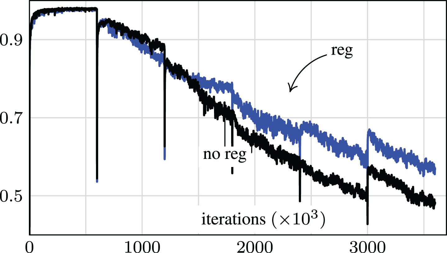
Permuted MNIST. We applied our method to the well-known permuted MNIST benchmark, initially proposed in [9]. In this benchmark, a sequence of tasks is derived from the standard MNIST dataset by randomly permuting the pixels of the MNIST images. For each task, a distinct permutation is applied, and within the same task, identical permutations are used for all MNIST digits. This setup simulates a continual learning scenario, where the data distribution undergoes substantial changes while transitioning between tasks. Our evaluation of performance focuses on cumulative accuracy on the test sets for each task. Let T₁, T₂, … denote the test sets for each task (with T _i obtained by applying the task-specific permutation to the MNIST test set). The cumulative accuracy for the t-th task is computed on T₁ ∪ T₂ ∪ … ∪ T _t . In Table 1, we present the final cumulative accuracy for an increasing number of tasks (up to 6 tasks). We compare results with and without the output-based regularization term. For each task, the learning procedure was executed for 10 epochs. The experiments utilizing our proposed regularization consistently achieve equal or higher performances compared to those without regularization. Notably, the regularization effect is more pronounced for a batch size of 1. In this scenario, the number of update iterations is higher due to the fixed number of epochs, resulting in a more pronounced forgetting effect in experiments without regularization. In Fig. 3, we visualize how the cumulative test accuracy evolves in relation to learning iterations (with a batch size of 1). As indicated by the results in Table 1, the regularized experiment’s accuracy curve consistently remains above the baseline curve during the majority of the training process, indicating significantly reduced forgetting. The accuracy drops in the curve correspond to task switches.

OPEN IN VIEWER

Fig. 3

Permuted MNIST. Cumulative test accuracy (in [0, 1]) as a function of the number of gradient-based-updates/iterations (batch-size is 1), with (blue) and without (black) the proposed output-based regularization term, in the permuted MNIST benchmark. The output-modulated update scheme yields better results than vanilla updates.

Non i.i.d. MNIST. The Non i.i.d. MNIST benchmark involves a supervised learning problem where MNIST digits are streamed one after another, sorted based on their labels. This setup introduces data dependency due to the ordering of the labels. The model learns from the stream without storing examples, making the batch size 1. The piece-wise constancy of labels requires avoiding overfitting on the current pattern while adapting to new labels. In this experiment, we set γ _k as a constant 1, and the modulating function ψ in Equation (18) is set to 0 if its value falls below a predetermined threshold θ (chosen as 0.001) to prevent model updates, as done in previous work [14]. Table 2 shows the results for various learning rates τ (Adam) using the small network. The output-based regularization policy proves beneficial when paired with a small learning rate, allowing the optimizer more flexibility to modulate the learning process. However, as the learning rate increases, the advantages diminish. This is because higher learning rates result in faster fitting to the target labels, leading to frequent output changes below the threshold θ. This, in turn, limits the number of parameter updates.

MNIST. This experiment diverges from our initial assumption, focusing on offline learning rather than the case-study’s online continual learning context. However, this initial exploration aims to determine whether the optimizer leads to performance drops or remains effective. The comparison of performances, measured by test set accuracy, is presented in Table 3 for different learning rates τ, batch sizes m, and neural architectures. The outcomes of this preliminary experiment suggest that no significant difference exists between the two methods, potentially indicating the applicability of our regularization term in classic offline learning tasks.

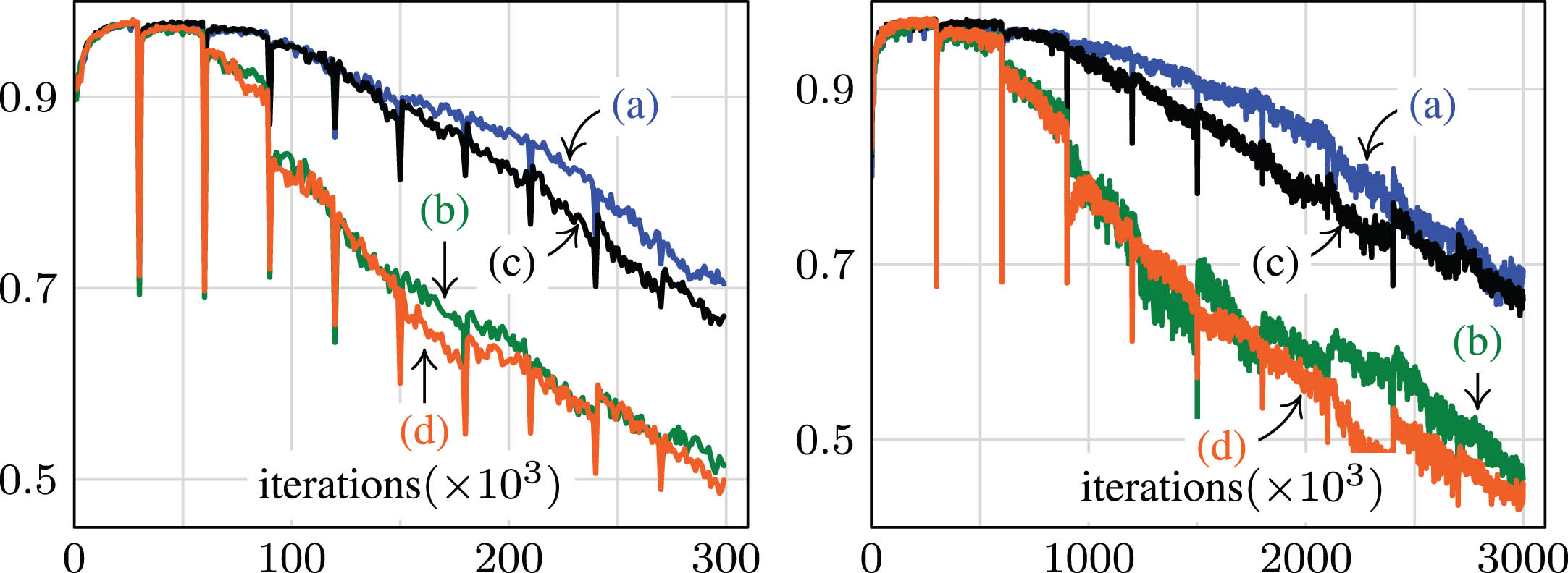
Progressive Permuted MNIST and CIFAR-10. While the Permuted MNIST benchmark is valuable for addressing specific aspects of continual learning, it raises concerns about its representativeness of real-world scenarios due to its dramatic shifts in data distribution between tasks. Our approach, which restrains updates on similar outputs, is expected to be particularly effective when data maintains cross-class resemblance. To assess this, we introduced a variant named Progressive Permuted MNIST, where the permutation of pixels that defines a new task is limited to a random subset of n_pix < 784 pixels. Two evaluation protocols were employed: Incremental and Non-incremental. In the Incremental protocol, new task data is generated by selecting n_pix pixels from the previous task’s data and applying a task-specific permutation only to these pixels. This approach leads to the possibility that the permutation introduced in task t could involve some pixels that were already permuted in task t - 1. On the other hand, the Non-incremental protocol involves permuting exactly tn_pix pixels of the original dataset for task t (until tn_pix ≥ 784, after which all pixels are permuted). Figure 4 showcases the differences between the two protocols. The Incremental scenario results in less drastic perturbations in inputs when transitioning between tasks, while the Non-incremental scenario quickly renders digits hard to recognize. In Fig. 5, we present the experimental results, considering 10 tasks and 5 epochs per task with n_pix = 500. Task switches are evident from the accuracy drops. While the output-based regularizer generally improves performance, it is particularly effective in the Incremental version of the progressive permuted MNIST dataset. In this Incremental scenario, moving from one task to another introduces gradual changes in the data distribution, leading to corresponding changes in the output of ν, which can be leveraged to modulate the update scheme. In contrast, the Non-incremental case has abrupt changes that are less suitable for effective modulation. Motivated by these results we tested the progressive incremental scenario on the more challenging CIFAR-10 dataset. As for the MNIST experiments the dataset for each new task is obtained from the previous one by a fixed permutation of a random subsample of the pixels. In Table 4 we show the results in a setting with 10 tasks, 5 epochs per task and n_pix = 50000. 6

OPEN IN VIEWER

Fig. 4

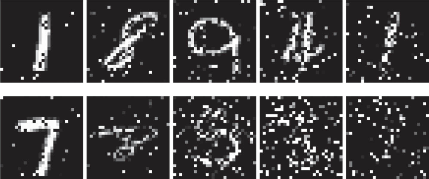
Progressive Permuted MNIST. First image of each new task (the task number increases going from left to right). Top-row: incremental protocol; bottom-row: non-incremental protocol. In the incremental case, digits are slowly made less distinguishable by a human. In the non-incremental scenario, digits are not recognizable (by a human) pretty soon, showing a more abrupt transition between consecutive tasks.

OPEN IN VIEWER

Fig. 5

Progressive Permuted MNIST. Cumulative test accuracy (in [0, 1]) as a function of gradient-based updates/iterations. The left-plots reports results for experiments run with batch size 10, while right-plots are about batch size 1. Within each plot we have: (a) with output-based regularization and incremental protocol; (b) with output-based regularization and non-incremental protocol; (c) without regularization and incremental protocol; (d) without regularization and with non-incremental protocol. The output-modulated update scheme yields more evident results in the incremental case, where the difference between consecutive tasks is evident but not excessively aggressive.

In this study, we explored the efficacy of leveraging Moreau-Yosida approximation to develop optimization methods for machine learning. We introduced a framework that provides a unified perspective on various gradient-based techniques, offering new interpretations and insights into their functioning. We applied the Moreau-Yosida view to the context of continual learning, creating a specialized output-modulated gradient-based step. This step inhibits parameter updates when the outputs of a neural network remain constant. Our experimental evaluation demonstrated the benefits of this method on datasets like permuted MNIST and progressively permuted MNIST. The advantages were more pronounced in scenarios with cross-task resemblance and non-i.i.d. streams. Furthermore, we showcased that the proposed update scheme remains valid for generic non-continual learning tasks.

Future research will explore the utilization of the Moreau-Yosida view to design novel optimizers for machine learning. This approach injects well-defined and understandable properties into the optimization problem, resulting in parameter update schemes with distinct characteristics.