Enhanced 3D parameterization for integrated shape synthesis by fitting parameter values to point sets

Abstract

Enhanced single-patch NURBS (Non-uniform rational B-splines) parameterization is developed based on fitting parameter values, capable of handling dynamically changing shapes. With respect to NURBS and T-splines, the proposed single-patch parameterizations results in lower dimensionality enabling optimizers to operate on geometric parameters. Avoiding subdivision surfaces and continuity problems for piecewise NURBS and reparameterizations for T-splines accelerates optimization. This parameterization may be an approximation or initial solution for piecewise NURBS and T-splines.

These numerical benefits are accomplished using a multi-stage methodology. An augmented set of fitting variables is formulated beyond the weight factors and control points with parameter values of data points. This augmented set is structured to possess reasonable dimensionality. The developed non-linear fitting includes gradient-based minimization with respect to the augmented set and evolutionary error minimization using external functions. The benefits and potential difficulties of the procedure are evaluated thoroughly.

The methodology is tested on engineering objects of high shape complexity and demonstrated to provide superior single-patch fitting performance compared to standard linear fitting methods.

The developed numerical approach provides for the aspired main objective which is sufficiently accurate and numerically efficient dynamic shape parameterizaton using a compact set of shape parameters.

Keywords

3D shape parameterization NURBS enhanced non-linear fitting integral dynamic surfaces

1. Introduction

1.1 Background, rationale and objectives

The computer-aided design (CAD) discipline has increasingly partnered with artificial intelligence methods and technologies, leading to entirely new perspectives in engineering design. Optimization-based re-design and reverse engineering of technical objects is one of the niches enabled recently by inheriting from the advanced 3D optical shape acquisition equipment and software. These technologies generally enable optimized performance and fast time-to-market. CAD systems have upgraded and evolved to being tools that are capable of modeling various objects and their coherence, restraints etc. Beyond the standard geometric primitives representing simple shapes, tools for free-form entities and point clouds have been developed and embedded as support for advanced geometric modeling.

At present, CAD tools support animations, simulations representing mechanisms and kinematic systems, systems engineering, practical modeling, modifications and distinctive particulars. External off-the-shelf or custom simulator applications can be coupled to provide additional functionality evaluations. Many engineering design problems involving CAD also rely on advanced external analysis methods, for example the finite element method in cases of requirements related to structural analysis. Occasionally, elementary optimization functionality is also supported. CAD systems are increasingly becoming comprehensive by integrating into product lifecycle management (PLM) systems which encompass standard CAD, CAM (manufacturing), CAE (engineering), reverse engineering, visualizations and other related activities.

A CAD model commonly involves many geometric primitives including complex ones such as NURBS, all combined (subject to constraint relationships) to jointly represent the respective engineering object.

Despite of advantages of using piecewise NURBS parameterization and T-splines in the fields of shape modeling and numeric analysis with respect to single-patch NURBS parameterization, those approaches suffer some drawbacks in dynamic aspects of the parameterizations. If we observe the results of those two approaches as input for an external numerical optimizer (CFD-computational fluid dynamics, FEA-finite element analysis, etc.) we are talking about dynamic processes of parameterization. During the process of dynamic parameterization, edges, peaks and other shape features may disappear and new ones may arise. The parameterization must be autonomously adaptable to such changes. This emphasizes the existing problems of subdivision surfaces and continuity at patch boundaries in the case of piecewise NURBS parameterization and completely new re-parameterization in the case of T-Splines. Therefore, in order to employ piecewise NURBS parameterization or T-splines in the process of dynamic parameterization, one has to be prepared for a long time period of execution of iterative and very complex numerical procedure.

We present enhanced single-patch NURBS parameterization based on fitting parameter values as a dynamic parameterization methodology. It is capable of handling dynamically changing shapes in optimization quasi-time iterations. It relies on papers [5, 36] which outline a parameterization based on fitting parameter values and classification of 3D shape deviation using feature recognition operating on parameterization control points.

This is related to 3D shapes acquired by applying optical 3D scanning [13], that include stereo-photogrammetry and triangulation [4, 22].

The proposed parameterization may be considered as an approximation or as an initial solution for the above mentioned approaches. Using single-patch parameterizations globally results in less dimensionality of the spatial solution what facilitates the use of an external numerical optimizer with results of the parameterization as input parameters. Furthermore, avoiding subdivision surfaces and continuity problems accelerates the process of optimizing shapes.

The term dynamic parameterization is in this paper related to shape optimization where the shape may change in optimization quasi-time. During this process, some geometric features may disappear and new one may appear. In such circumstances, adequate representation of the changing geometry is a prerequisite for satisfactory numerical precision and convergence of the optimization procedure. Advanced processing of the geometric information should establish a foundation for shape-related considerations including feature recognition and classification.

The motivation of this paper and its primary objectives are straightforward. In engineering optimization (especially when using genetic algorithms) it is of utmost importance to model shapes using sparing sets of shape parameters as the number of shape parameters maps into the dimensionality of the search space. This paper is motivated by the aspiration to avoid numerical procedures which use geometric information only and make no use of topologic information. Such methods, for example the ICP algorithm, do not converge globally or rely on genetic algorithms throughout the procedure. The overall objective of the proposed approach is to develop a new fitting procedure capable of representing complex geometries very accurately.

This paper, after reviewing the relevant literature and providing the basic terms of NURBS, develops the key elements of the proposed procedure including:

•
Obtaining a structured matrix form of the geometry,
•
Formulating an augmented set of fitting variables including the control points, weight factors and parameter values of data points,
•
Structuring and reduction of the augmented set towards moderate dimensionality,
•
Developing a gradient-based non-linear fitting procedure with respect to the augmented set,
•
Developing an evolutionary fitting error minimization using external functions.

whereby the benefits and potential difficulties of the developed procedure are critically assessed. This is accompanied by several complex engineering objects serving as test-cases for the deveoped methodology.
1.2 Related work and literature

CAD models largely suffer from difficulties in sharing data among heterogeneous CAD systems. Zhang et al. [37] describe this problem and outline a new asymmetric strategy to enrich the theory of feature-based interoperability. Li et al. [16] contribute to this issue with a method to gain one-dimensional topological entity matching. Fortunately, the proposed parametric model does not suffer from this problem because it is mathematically well defined. As long as we do not extend the model to multi-patch NURBS or T-spline models, we do not need to care about this matter. Nevertheless, operating directly on systems of CAD geometric primitives is not suitable for many advanced applications such as shape optimization of engineering objects or shape synthesis in general. Non-uniform rational B-splines (NURBS) are the current standard technology that is used by CAD systems to represent free-form geometries. These entities provide for rather generic CAD model transformations and modifications using the corresponding operators which manipulate the model parameters.

Because of the NURBS restriction to a regular grid parameter domain and local refinement by inserting (multiple) knots which leads to a rising number of control points, the approaches which use integral compact (single-patch) NURBS parameterizations have found less application in the field of shape modeling and numerical analysis. Many authors resort to the use of piecewise NURBS parameterizations as well as the latest generally accepted mathematical model (T-splines). This approach avoids the main disadvantages of using single-patch NURBS parameterizations in shape modeling and numerical analysis.

Except for advantages and disadvantages of using piecewise NURBS parameterization and T-splines with respect to single-patch NURBS parameterization, several authors also outline the advantages of applying piecewise NURBS parameterization with respect to T-splines and vice versa. Riffnaller-Schiefer et al. [25] presented isogeometric shell analysis based on a subdivision algorithm that generalises NURBS to arbitrary topology. In terms of choosing a model, the authors draw attention to the lack of linear independence of the basic functions of the T-intersection and therefore consider the subdivision surfaces as the better choice than T-splines for isogeometric analysis. Using multiple knots results in adding columns or rows of control points which corresponds to a rising dimensionality of the spatial solution. The authors point out that if multiple knots are not supported, the boundaries cannot be parameterized correctly for the required symmetry conditions. Dimitri et al. [7] applied T-spline-based isogeometric analysis to frictionless contact problems between deformable bodies in the context of large deformations. The authors note the disadvantages of multiple NURBS patches such as discontinuity across patch boundaries, global refinement with respect to T-splines and a large percentage of NURBS control points which are needed only to satisfy topological constraints. Nguyen et al. [21] present Nitche’s method to couple non-conforming two and three-dimensional NURBS patches in the context of isogeometric analysis. The authors mention the benefits of using coupled patches with respect to single patch parameterization. Li et al. [17] established several fundamental properties of analysis-suitable T-splines which are important for design and analysis. The benefits of T-splines were used by Dimitri et al. [8] in NURBS and T-spline-based isogeometric analysis for cohesive zone modeling of interface debonding. Vučina et al. [35] have applied chained Bezier surfaces in shape optimization related parameterizations.

Campomanes-Alvarez et al. [3] use genetic algorithms and simplify open 3D meshes while preserving the accuracy, especially in areas of geometrical features. Extraction of unique feature related information is also a demanding task in the area of biometrics technologies. As a base for using the Hidden Markov Model (HMM), Meraoumia et al. [20] use VARiance measures (VAR) for invariant rotation and PCA (Principal Component Analysis) for compressing information regarding geometric features. Seifert et al. [33] outline the combinations of two sampling techniques for binary classification models. This classification can be utilized should a geometric feature be used in related methods. Elaborate overviews of various approaches in geometric modeling and parameterization regarding optimization and shape modeling are found in [27, 28]. Along with optimization and optimal design, different mathematical processing and numerical approaches are used in [6, 24, 29]. Distinct approaches to shape modeling exhibit significant impact on subsequent numerical analysis. In order to accomplish the necessary performance and functionality, the corresponding numerical approach and simulation procedures should be related with shape modeling. An adequate approach needs to promote efficient coupling of the geometric model and the simulation model. Geometric objects which constitute the overall shape model include simple primitives such as spheres and cylinders, but also involve complex mathematical curves and surfaces like B-splines and NURBS [2, 34], which provides for generality in modeling complex shape [1, 12, 26]. Recent improvements in CAD technology have resulted in advanced and powerful applicability. In [18, 19, 23, 30], the need to have parameterizations of the resulting point clouds as mathematical surfaces is outlined. Further aspects of best-fitting 3D mathematical surfaces such as B-spline and NURBS surfaces related to data-sets acquired by measurement and numerically generated surfaces is emphasized in [9, 10, 11, 15, 18, 23].

The papers [14, 31] consider shape optimization of structures using evolutionary algorithms which in fact combines sizing, shape and topology optimization. Cost-based optimization of space structures subject to different objectives and design code constraints was presented in [32] using parallelized GA algorithms.

2. Development of an efficient parameterization

The NURBS surface is defined by its control points, weight factors, degrees of polynomials and the set of knots,

$\displaystyle{\bm{C}}\left(u,v\right)=$ (1) $\displaystyle\frac{\sum\limits_{i_{0}=0}^{n_{0}}\sum\limits_{i_{1}=0}^{n_{1}}{% N_{i_{0},p_{u}}(u)N_{i_{1},p_{v}}(v)w_{i_{0}i_{1}}{\bm{Q}}_{i_{0}i_{1}}}}{\sum% \limits_{i_{0}=0}^{n_{0}}\sum\limits_{i_{1}=0}^{n_{1}}{N_{i_{0},p_{u}}(u)N_{i_% {1},p_{v}}(v)w_{i_{0}i_{1}}}}\in\mathbb{R}^{3}$

where $n_{0},n_{1}$ are the numbers of the control points, $N_{i_{0},p_{u}}(u)$ and $N_{i_{1},p_{v}}(v)$ are the basic B-spline functions of degrees ${p_{u},p}_{v}\in\mathbb{N}$ defined by

$\displaystyle N_{i,0}(u)=\begin{cases}1,&\bar{u}_{i}\leqslant u\leqslant\bar{u% }_{i+1}\\ 0,&\rm else\\ \end{cases},$ $\displaystyle N_{i,p}(u)=\frac{u-\bar{u}_{i}}{\bar{u}_{i+p}-\bar{u}_{i}}N_{i,p% -1}(u)+$ (2) $\displaystyle\qquad\qquad∼{}\frac{\bar{u}_{i+p+1}-u}{\bar{u}_{i+p+1}-\bar{u}_{% i+1}}N_{i+1,p-1}(u).$

The knots $\bar{u}_{i}\in[0,1]$ as part of the basic B-spline functions we set as

$\displaystyle\bar{\bm{u}}=\left\{\underbrace{0,\ldots,0}\limits_{p+1},\bar{u}_% {i+p},\ldots,\bar{u}_{n-p-1},\underbrace{1,\ldots,1}\limits_{p+1},\right\},$ $\displaystyle\left\{\bar{u}_{i}=\frac{i}{n}\right\}_{i=p+1}^{n-p-1}.$ (3)

The matrix ${\bm{Q}}$ given by

$\displaystyle{\bm{Q}}=\begin{bmatrix}{\bm{Q}}_{00}&\ldots&{\bm{Q}}_{0n_{1}}\\ \vdots&\ddots&\vdots\\ {\bm{Q}}_{n_{0}0}&\ldots&{\bm{Q}}_{n_{0}n_{1}}\\ \end{bmatrix}\in\mathbb{R}^{3(n_{0}+1)\times(n_{1}+1)}$ (4)

contains the set of control points, and the matrix ${\bm{W}}$

$\displaystyle{\bm{W}}=\begin{bmatrix}w_{00}&\ldots&w_{0n_{1}}\\ \vdots&\ddots&\vdots\\ w_{n_{0}0}&\ldots&w_{n_{0}n_{1}}\\ \end{bmatrix}\in\mathbb{R}^{(n_{0}+1)\times(n_{1}+1)}$ (5)

denotes the weight factors. For arbitrary arguments $u$ and $v\in[0,1]$ , the vector ${\bm{C}}(u,v)$ represents the corresponding point lying on the NURBS surface.

Fitting a NURBS surface with matrix topology can be viewed as a procedure of deforming a flexible plate until it assumes the required shape. The control points of the NURBS surface can be perceived as vertices at which forces are applied which deform the plate accordingly. The extent of local deformation is determined by the degrees of the surface, and the intensity of local deformation is controlled by the homogeneous terms of the NURBS surface.

This analogy reveals that the flexible plate cannot be deformed at a point without affecting its surroundings, and it is a smooth function which describes this deformation. The same applies for the NURBS surface where the change of shape is smooth and encompasses a certain area regardless of the mechanism of change, whether it was imposed by control points, homogenous terms, parameter values or knot values.

The notion of fitting a NURBS surface to some given geometry with matrix topology implies in this paper that the geometry can be written in matrix form according to Eq. 6.

In order to obtain a matrix topology, we apply a projection of shape into a rectangular domain in all examples. The projection into a rectangular domain is generally an extensive and demanding topic and hence a subject of future work, while only outlined in this paper.

3. Obtaining a structured form of the original object geometry

In this paper the term fitting to ‘geometry’ implies the ‘geometry’ to be a point cloud resulting for example from 3D scanning of some engineering object. An example of such geometries is shown in Fig. 1 which displays a point cloud of a small sailing boat hull with a number of cross-sections.

$\displaystyle{\bm{P}}=\begin{bmatrix}{\bm{P}}_{00}&\ldots&{\bm{P}}_{0m_{1}}\\ \vdots&\ddots&\vdots\\ {\bm{P}}_{m_{0}0}&\ldots&{\bm{P}}_{m_{0}m_{1}}\\ \end{bmatrix}\in\mathbb{R}^{3(m_{0}+1)\times(m_{1}+1)}$ (6)

Figure 1.

Matrix form of geometric data obtained by intersecting the point cloud by (a) parallel sections, (b) sections from a pole at different angles.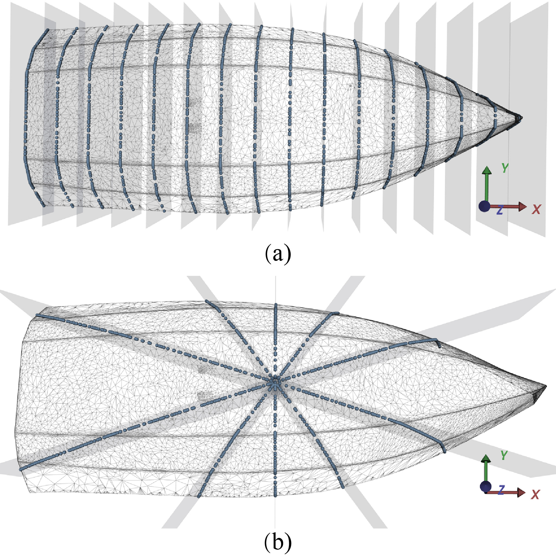

The matrix data-set topology consists of $(m_{0}+1)$ sections with $(m_{1}+1)$ points in each section. The number of rows ${(m}_{0}+1)$ of the matrix ${\bm{P}}$ corresponds to the number of parallel sections in Fig. 1(a). Initially, by virtue of intersecting the geometry by planes, the sections contain 3D points where the plane intersects the edges of the triangulated surface (mesh of planar faces). Such sections generally involve different multitudes of points per section. In order to be recorded in the form of matrix ${\bm{P}}$ , all the sections must have the same number of points equal to $(m_{1}+1)$ . The geometric topology of the triangulated surface, i.e. the connectivity of intersected edges makes the sections also represent contours. This implies that there exists an increasing algorithmic device amongst the points of the contour such that a simple procedure is possible to select ${(m}_{1}+1)$ points for each section. If $\left\{{\bm{P}}_{i}^{O}\right\}_{i=0}^{n}$ denotes the original $(n+1)$ points of an individual contour before intersecting and $\left\{{\bm{P}}_{k}^{C}\right\}_{k=0}^{m_{1}}$ designates the new $(m_{1}+1)$ points at the same contour, then the following conditions apply for each new point ${\bm{P}}_{k}^{C}$ :

There exists an $i$ such that ${\bm{P}}_{k}^{C}\in[{\bm{P}}_{i}^{O},{\bm{P}}_{i+1}^{O}]$ ,

$\displaystyle\sum\nolimits_{j=0}^{i}\left\|{\bm{P}}_{j+1}^{O}-{\bm{P}}_{j}^{O}% \right\|+\left\|{\bm{P}}_{i}^{O}-{\bm{P}}_{k}^{C}\right\|$ $\displaystyle=k\frac{\sum_{j=0}^{n}\left\|{\bm{P}}_{j+1}^{O}-{\bm{P}}_{j}^{O}% \right\|}{m_{1}+1}.$ (7)

The expression Eq. 7 aims at finding the respective interval where the point ${\bm{P}}_{k}^{C}$ is located whereby $(i-1)$ whole intervals and a part of the $i$ -th are cumulated, which is a simple single-loop procedure.

The pursuit of deriving the sections matrix ${\bm{P}}$ in Eq. 6 belongs to topology optimization and represents a problem in itself. Nevertheless, topology optimization as an element in best-fitting of this type introduces some major advantages. One of such benefits are numerically good initial solutions both for gradient methods and genetic algorithms. The matrix form of the geometry also enables mature and well-tested algorithms borrowed from image processing to be engaged, which makes best-fitting faster and numerically more stable.

The procedure of fitting a NURBS surface to the geometry given by the sections matrix ${\bm{P}}$ assigns a pair of parametric values $u_{j_{0}j_{1}}$ and $v_{j_{0}j_{1}}\in[0∼{}∼{}1]$ to each point ${\bm{P}}_{j_{0}j_{1}}$ such that

$\displaystyle{\bm{C}}(u_{j_{0}j_{1}},v_{j_{0}j_{1}})\to{\bm{P}}_{j_{0}j_{1}}$ (8)

where ${\bm{C}}(u_{j_{0}j_{1}},v_{j_{0}j_{1}})$ is the point on the NURBS surface Eq. 1 which is to be determined by fitting to the given geometry. In Eq. 8, the symbol $\to$ reads ‘corresponds to’. If the NURBS surface has sufficient internal degrees of freedom, Eq. 8 can become interpolation in which case the symbol $\to$ evolves to the equality symbol $=$ .

For easier orientation in the case of the example in Fig. 1, the parameter $u$ can be associated with variation of the positions of sections and $v$ with the position along the sections.

The corresponding parametric values can be assembled in matrix form

$\displaystyle{\bm{U}}=\begin{bmatrix}u_{00}&\ldots&u_{0m_{1}}\\ \vdots&\ddots&\vdots\\ u_{m_{0}0}&\ldots&u_{m_{0}m_{1}}\\ \end{bmatrix}\in\mathbb{R}^{(m_{0}+1)\times(m_{1}+1)}$ (9)

and

$\displaystyle{\bm{V}}=\begin{bmatrix}v_{00}&\ldots&v_{0m_{1}}\\ \vdots&\ddots&\vdots\\ v_{m_{0}0}&\ldots&v_{m_{0}m_{1}}\\ \end{bmatrix}\in{\mathbb{R}}^{\left(m_{0}+1\right)\times\left(m_{1}+1\right)}$

In terms of easier association of Eq. 9 with the example in Fig. 1, the rows in ${\bm{U}}$ and ${\bm{V}}$ are related to different sections, and the columns to different points along sections.

Generally, the NURBS surface which represents the geometry of the sections matrix ${\bm{P}}$ must minimize the error function

$\displaystyle{\bm{E}}\left({\bm{U},\bm{V},\bm{Q},\bm{W}}\right)$ $\displaystyle=\frac{1}{2}\sum_{j_{0}=0}^{m_{0}}\sum_{j_{1}=0}^{m_{1}}\left\|{% \bm{C}}(u_{j_{0}j_{1}},v_{j_{0}j_{1}})-{\bm{P}}_{j_{0}j_{1}}\right\|^{2}$ (10)

which constitutes a least-squares problem. Minimizing the error function Eq. 10 reduces the cumulative sum of distances between the geometry ${\bm{P}}_{j_{0}j_{1}}$ and the corresponding points on the NURBS surface ${\bm{C}}(u_{j_{0}j_{1}},$ $v_{j_{0}j_{1}})$ . An individual distance is the norm of the individual error vector, visualized for example by $e_{1}$ in Fig. 2. By minimizing the error function

$\displaystyle{\bm{E}}^{\text{actual}}\left({\bm{Q},\bm{W}}\right)$ $\displaystyle=\frac{1}{2}\sum_{j_{0}=0}^{m_{0}}\sum_{j_{1}=0}^{m_{1}}% \underbrace{\min}\limits_{u,v}{\left\|{\bm{C}}(u,v)-{\bm{P}}_{j_{0}j_{1}}% \right\|}^{2}$ (11)

we calculate the actual geometric error by finding the closest point on the surface for each point ${\bm{P}}_{j_{0}j_{1}}$ , as indicated by $e_{2}$ in Fig. 2. We refer to the difference between the two error functions as the topological component of the error and, generally, optimization based on fitting parameter values we call topological optimization.

Figure 2.

Two ways of determining the local fitting error: 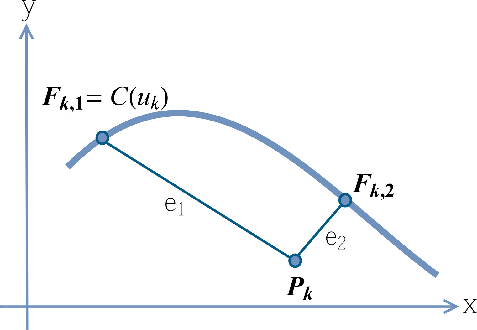$e_{1}$ $:=$ $|{\bm{P}}_{k}-{\bm{C}}(u_{k})|$ obtained directly from the least squares method with assigned $u_{k}$ , $e_{2}:=\min_{u}|{\bm{P}}_{k}$ $-$ ${\bm{C}}(u)|$ obtained from actual error Eq. 11.

The procedure developed in this paper introduces topological optimization with respect to the parameter values ${\bm{U}}$ and ${\bm{V}}$ in Eq. 9 in the context of best-fitting to point clouds. This formulation has the consequence of reducing the topological component in the overall error. Based on numerical experiments with test-cases, the topological error generally dominates the actual geometric error. Consequently, most optima with respect to topological degrees of freedom ( ${\bm{U}}$ and ${\bm{V}}$ ) are numerically acceptable and can be accepted as general optima, while the inverse may not hold.

Figure 3 shows a NURBS surface which ‘numerically ideally’ represents the given (shape) geometry ${\bm{P}}$ , Eq. 6. The term ‘ideally’ is here defined as: “the offset between the given shape and the NURBS surface is below the preset tolerance and tends to zero, given the minimum number of control points necessary to achieve the given error margin”.

Figure 3.

(a) NURBS surface ‘ideally’ representing the geometry; (b) points of the ‘ideal’ NURBS surface and simultaneously points of the triangulated point cloud obtained by inserting corresponding parameter values into the NURBS surface definition Eq. 1.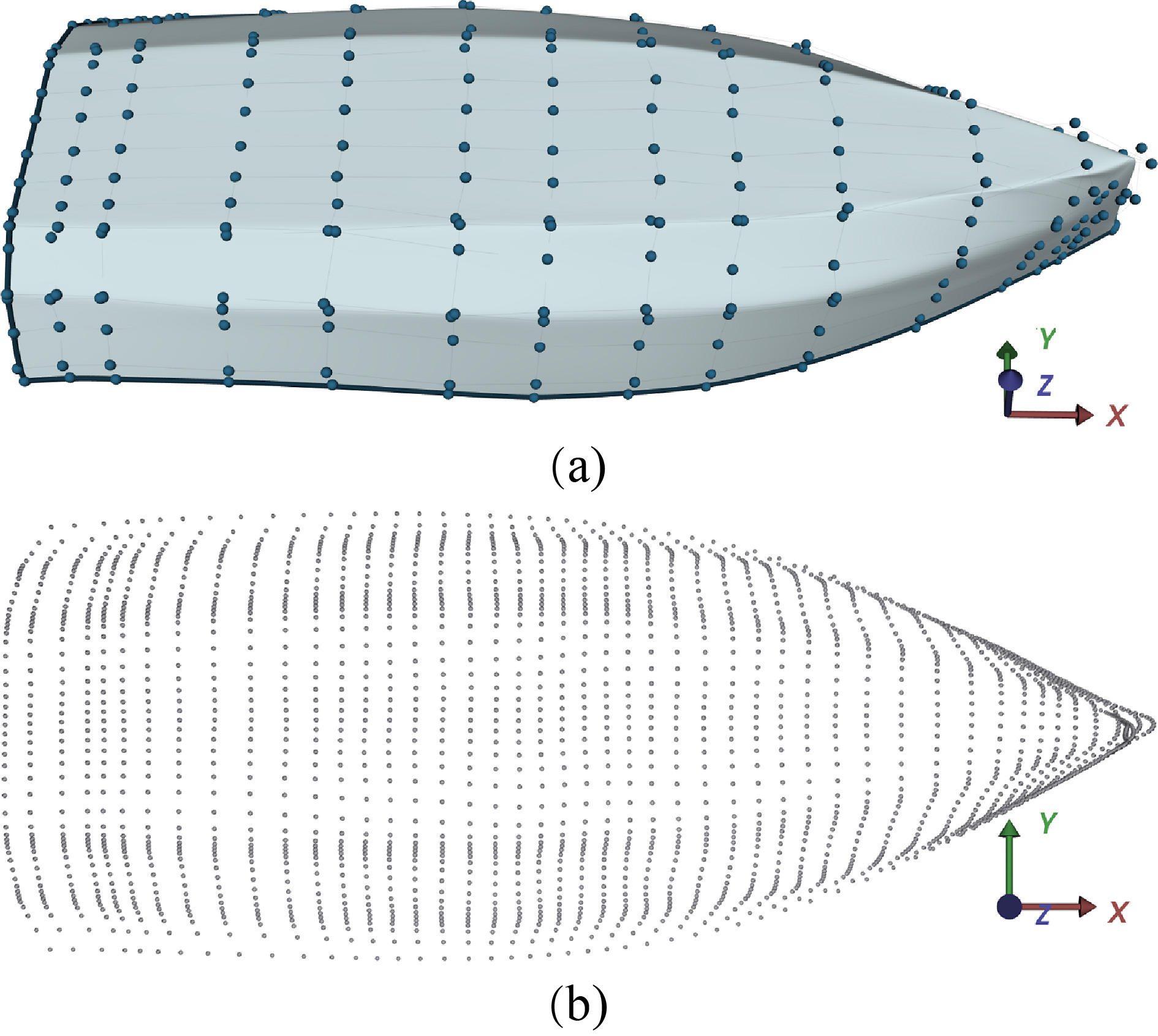

Figure 3 shows the points of the ideal surface obtained for the parameter values according to Eq. 12. The NURBS surface in Fig. 3 is fitted to the geometry, the term geometry referring to the point cloud obtained by 3D scanning of a sailing boat hull. The cloud is subsequently processed and formatted to matrix form Eq. 6 as explained earlier related to Eq. 7, given the parameter values according to

$\displaystyle\left\{u_{j_{0}0}=u_{j_{0}1}=\ldots=u_{j_{0}m_{1}}:=\frac{j_{0}}{% m_{0}}\right\}_{j_{0}=0}^{m_{0}}$

and

$\displaystyle\left\{v_{{0j}_{1}}=v_{{1j}_{1}}=\ldots=v_{m_{0}j_{1}}:=\frac{j_{% 1}}{m_{1}}\right\}_{j_{1}=0}^{m_{1}}.$ (12)

Chord-length based assignment of parameter values could also be applied.

The 3D points obtained this way can also be viewed as the sections matrix ${\bm{P}}$ since they are also points of the triangulated point cloud due to the ‘ideal’ description of the geometry. This relates to the concept of interpolation where the NURBS surface has sufficient degrees of freedom to ‘pass through’ the given geometry ${\bm{P}}$ .

4. Development of an enhanced best-fitting method

4.1 Background

If the section matrix ${\bm{P}}$ would contain points which belong to the ‘ideal’ NURBS surface and the corresponding parameter values would be obtained for those points according to Eq. 12, then the best-fitted NURBS surface would result from solving a simple linear problem [10]. Nevertheless, it is unlikely that the section matrix ${\bm{P}}$ obtained by applying parallel sections coincides with the points of the ideal NURBS surface and simultaneously the triangulated point cloud, Fig. 4(b). During the fitting procedure, each point ${\bm{P}}_{j_{0}j_{1}}$ is assigned a pair $u_{j_{0}j_{1}}$ and $v_{j_{0}j_{1}}\in[0∼{}∼{}1]$ such that Eq. 8holds. Figure 4(a) shows the sections matrix ${\bm{P}}$ obtained by parallel sections and in particular the $j_{0}$ -th column whose values $\left\{u_{j_{0}j_{1}}\right\}_{j_{1}=0}^{m_{1}}$ obtained using Eq. 12 have the value 0.4.

Figure 4.

Difference in determining the $\bm{P}$ matrix, (a) $j_{0}$ -th column obtained by the intersection procedure of Eq. 7; (b) $j_{0}$ -th column resulting from introducing the values Eq. 12 into the NURBS definition Eq. 1.

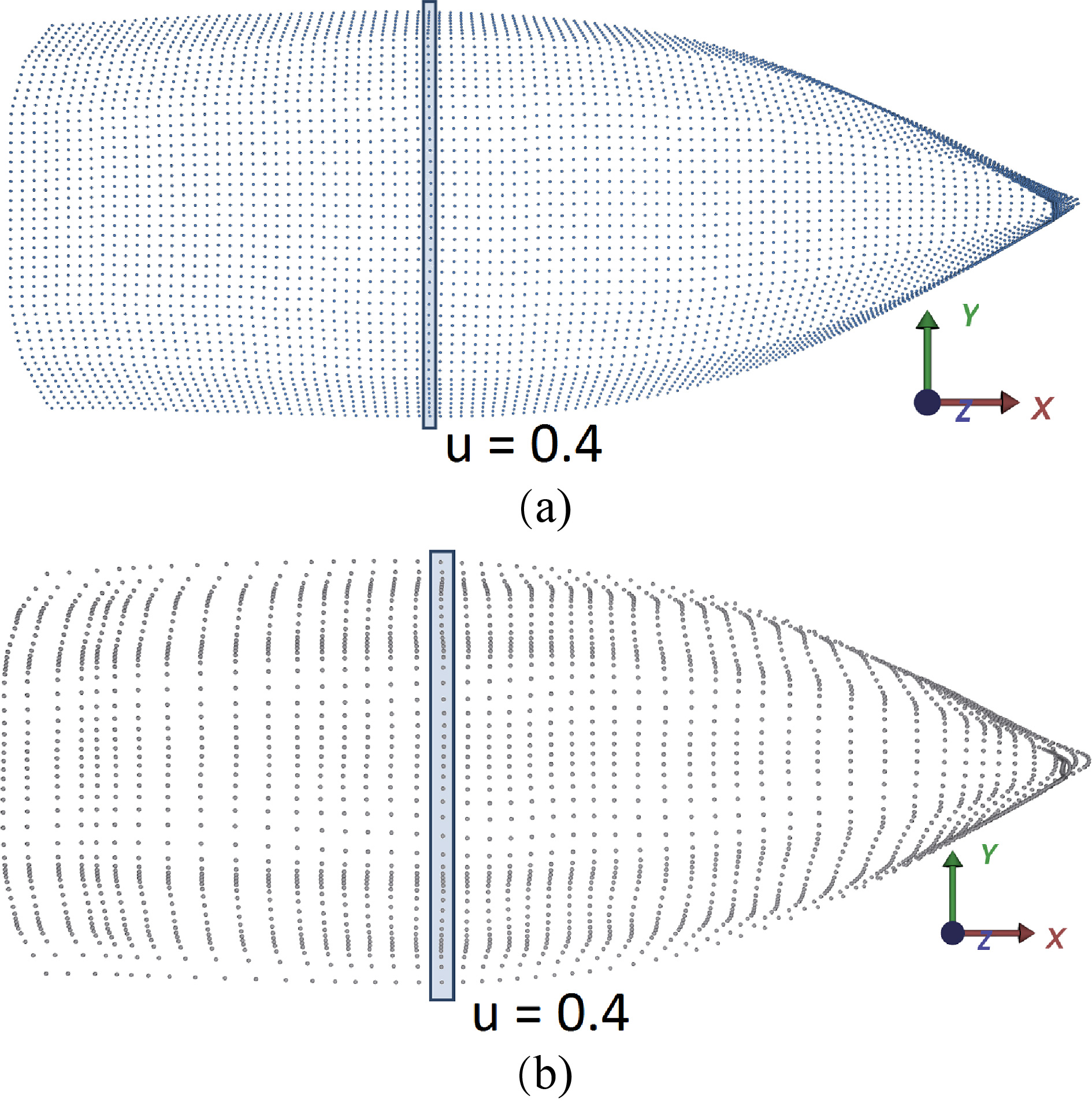
On the other hand, Fig. 4(b) shows the points of the ideal NURBS surface and the $j_{0}$ -th column obtained from the NURBS definition for $\left\{u_{j_{0}j_{1}}\right\}_{j_{1}=0}^{m_{1}}=0.4$ . Although the corresponding values of $u_{j_{0}j_{1}}$ are the same for both columns, the columns in 3D do not coincide.

4.2 Data points parameter values as additional fitting variables

The ambition of this paper is to enhance the best–fitting procedure as follows. The developed procedure intends to engage the matrices of parameter values ${\bm{U}}$ and ${\bm{V}}$ Eq. 9 as additional best-fitting variables in addition to the standard best-fitting variables which comprise of the control points ${\bm{Q}}$ and homogeneous terms ${\bm{W}}$ . The idea is to compensate the error (Fig. 4) introduced by formulating the matrix ${\bm{P}}$ using parallel sections.

Figure 5 visualizes the respective ${\bm{U}}$ and ${\bm{V}}$ matrices for the selected values Eq. 12. The graphical visualization of the ${\bm{U}}$ and ${\bm{V}}$ matrices is used for easier presentation of the fitting procedure.

Figure 5.

Graphical presentation of the 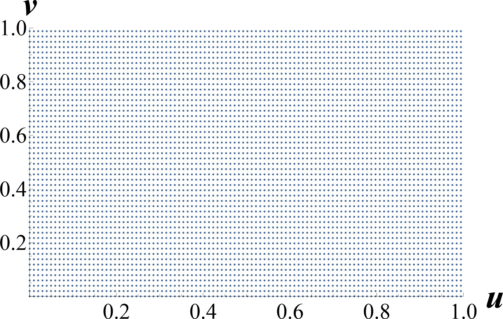$\bm{U}$ and $\bm{V}$ matrices.

However, any optimization including best-fitting should keep the number of degrees of freedom at the reasonable minimum for computational reasons. In the error function Eq. 10, the number of control points and hence also the homogenous terms is $\left(n_{0}+1\right)\times\left(n_{1}+1\right)$ . It is commonly pre-set based on experience. This count of the corresponding best-fitting degrees of freedom is not excessively high.

Nevertheless, the size of the section matrix ${\bm{P}}$ can be very large, leading to correspondingly large ${\bm{U}}$ and ${\bm{V}}$ matrices. Having this in mind, treating all elements of the ${\bm{U}}$ and ${\bm{V}}$ matrices as best-fitting degrees of freedom (on top of ${\bm{Q}}$ and ${\bm{W}}$ ) is not reasonable. There is another motivation not to include all elements of ${\bm{U}}$ and ${\bm{V}}$ as independent best-fitting variables. The changes in ${\bm{U}}$ and ${\bm{V}}$ must be smooth and the respective sequences of values need to be ordered. An isolated change of any element of these matrices without associated changes in its neighborhood leads to geometric singularity as indicated in the example given later.

4.3 Structuring the set of augmented best-fitting variables

These circumstances provide the rationale behind the original approach proposed and developed here. In the proposed approach, the matrices of parameter values ${\bm{U}}$ and ${\bm{V}}$ are formed as sums of two respective matrices,Eqs 13 and 14. The first matrices have the same number of degrees of freedom as the initial matrices ${\bm{U}}$ and ${\bm{V}}$ , whilst the second matrices are obtained by repeating a column in ${\bm{U}}$ and a row in ${\bm{V}}$ . Accordingly, ${\bm{U}}$ and ${\bm{V}}$ can be decomposed as

$\displaystyle\begin{bmatrix}u_{00}&\ldots&u_{0m_{1}}\\ \vdots&\ddots&\vdots\\ u_{m_{0}0}&\ldots&u_{m_{0}m_{1}}\\ \end{bmatrix}=\begin{bmatrix}c^{u}_{00}&\ldots&c^{u}_{0m_{1}}\\ \vdots&\ddots&\vdots\\ c^{u}_{m_{0}0}&\ldots&c^{u}_{m_{0}m_{1}}\\ \end{bmatrix}+$ $\displaystyle\begin{bmatrix}u_{0}&\ldots&u_{0}\\ \vdots&\ddots&\vdots\\ u_{m_{0}}&\ldots&u_{m_{0}}\\ \end{bmatrix},∼{}\text{i.e.}$ $\displaystyle{\bm{U}}={\bm{C}}^{u}+\left[\underbrace{\bm{u}\bm{u}\ldots\bm{u}}% \limits_{m_{1}+1}\right]={\bm{C}}^{u}+{\bm{K}}^{u},$ (13)

and

$\displaystyle\begin{bmatrix}v_{00}&\ldots&v_{0m_{1}}\\ \vdots&\ddots&\vdots\\ v_{m_{0}0}&\ldots&v_{m_{0}m_{1}}\\ \end{bmatrix}=\begin{bmatrix}c^{v}_{00}&\ldots&c^{v}_{0m_{1}}\\ \vdots&\ddots&\vdots\\ c^{v}_{m_{0}0}&\ldots&c^{v}_{m_{0}m_{1}}\\ \end{bmatrix}+$ $\displaystyle\begin{bmatrix}v_{0}&\ldots&v_{m_{1}}\\ \vdots&\ddots&\vdots\\ v_{0}&\ldots&v_{m_{1}}\\ \end{bmatrix},∼{}\text{i.e.}$ $\displaystyle{\bm{V}}={\bm{C}}^{v}+\left[\underbrace{\bm{v}\bm{v}\ldots\bm{v}}% \limits_{m_{0}+1}\right]^{\tau}={\bm{C}}^{v}+{\bm{K}}^{v}.$ (14)

The developed procedure proposes that proceeding from the linear best-fitting solution (Fig. 6) and based on Eqs 13 and 14, the fitting procedure can be continued and augmented by non-linear best fitting:

(a) 1.

Using gradient methods in best-fitting with respect to vectors of parameter values ${\bm{u}}\in\mathbb{R}^{m_{0}+1}$ and ${\bm{v}}\in\mathbb{R}^{m_{1}+1}$ in the matrices ${\bm{K}}^{u}$ and ${\bm{K}}^{v}$ in Eqs 13 and 14.

Using genetic algorithms in best-fitting with respect to matrices ${\bm{C}}^{u}$ and ${\bm{C}}^{v}\!\in\!\mathbb{R}^{(m_{0}+1)\times(m_{1}+1)}$ in Eqs 13 and 14.

The latter (b) is implemented by applying external functions which use only a few internal fitting parameters to impose the respectively available modes of changing the elements of ${\bm{C}}^{u}$ and ${\bm{C}}^{v}$ .

The advantage of this procedure is a sparing number of additional degrees of freedom with respect to standard linear best-fitting, and a much smaller number than if elements of ${\bm{U}}$ and ${\bm{V}}$ would have been independent best-fitting variables. In the step (a), optimizing by gradient non-linear methods with respect to the vectors of parameter values in Eqs 13 and 14 ( ${\bm{u}}\in\mathbb{R}^{m_{0}+1}$ , ${\bm{v}}\in\mathbb{R}^{m_{1}+1}$ ) instead of optimization with respect to full matrices ${\bm{C}}^{u}$ and ${\bm{C}}^{v}\in\mathbb{R}^{(m_{0}+1)\times(m_{1}+1)}$ reduces the number of best-fitting variables from $(m_{0}+1)\times(m_{1}+1)$ to ${(m}_{0}+m_{1}+2)$ .

Nevertheless, the proposed reduction of the number of degrees of freedom also leads to a loss of globality of the optimization procedure. Moreover, the symmetrical parameter values (equal columns/rows inEqs 13, 14 in optimization) are more suitable for engineering objects with symmetrical shape than for general shapes.

Figure 6.

Solution of the linear fitting problem [10], B-spline surface and control points.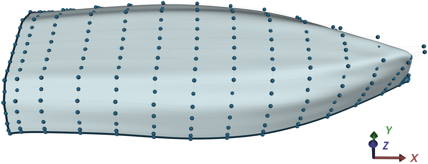

The step (b) of the procedure is proposed in order to recover the globality of optimization and improve fitting for non-symmetrical objects. In the step (b), optimization of the matrices ${\bm{C}}^{u}$ and ${\bm{C}}^{v}$ using genetic algorithms is implemented by applying external functions. This reduces the associated number of degrees of freedom from $(m_{0}+1)\times(m_{1}+1)$ to the respective number of internal degrees of freedom of those respective functions.

The step (b) apparently also leads to the loss of globality of optimization since the elements of the matrices ${\bm{C}}^{u}$ and ${\bm{C}}^{v}$ are no longer autonomous degrees of freedom. However, as stated earlier, the change of parametric values needs to be smooth and extend across a certain area around the point of change. Accordingly, external functions controlled by the genetic algorithms can be incorporated by any smooth function changing the values of the matrices ${\bm{C}}^{u}$ and ${\bm{C}}^{v}$ , provided it preserves the monotonously growing functional relationship for the matrix values. Fourier functions, radial-basis functions, B-splines, etc. could all be potential candidates for this assignment. Because of the resulting algorithmic complexity, these functions should possess as few as possible internal degrees of freedom. In the specific case that follows, the number of degrees of freedom of the external functions equals three.

4.4 Non-linear gradient (LM) best-fitting based on augmented set of variables

Based on the proposed form of the matrices of parameter values, the error function can now be re-written as:

$\displaystyle{\bm{E}}(\bm{u},\bm{v},\bm{Q},\bm{W})=$ (15) $\displaystyle\frac{1}{2}\sum_{j_{0}=0}^{m_{0}}\sum_{j_{1}=0}^{m_{1}}\left\|{% \bm{C}}(c^{u}_{j_{0}j_{1}}{+}u_{j_{0}},c^{v}_{j_{0}j_{1}}{+}v_{j_{1}}){-}{\bm{% P}}_{j_{0}j_{1}}\right\|^{2}$

In the proposed approach, fitting with respect to the ${\bm{u}}$ and ${\bm{v}}$ vectors in ${\bm{K}}^{u}$ and ${\bm{K}}^{v}$ introduces equal changes for the rows of the ${\bm{U}}$ matrix and columns of the ${\bm{V}}$ matrix, which may initially seem as a loss of generality. Nevertheless, engineering objects tend to possess sharp edges which commonly have straight shapes. Fitting NURBS surfaces to such geometries implies aggregation of the control points in the vicinity of the edges such that they also lie along straight lines, which is in favor of the column-wise and row-wise change in the ${\bm{U}}$ and ${\bm{V}}$ matrices respectively.

Setting the ${\bm{u}}$ and ${\bm{v}}$ vectors to zero-vectors makes ${\bm{U}}$ equal to ${\bm{C}}^{u}$ and ${\bm{V}}$ to ${\bm{C}}^{{\bm{v}}}$ , and the error function Eq. 15 goes back to Eq. 10. In order to obtain the initial solution, the homogeneous term ${\bm{W}}$ is commonly set to the unit matrix, making the NURBS surface degrade to the Bspline surface. By applying parallel sections (Fig. 1(a)), the sections matrix ${\bm{P}}$ is initialized as shown in Fig. 4(a), whereby the initial values of the matrices ${\bm{U}}$ and ${\bm{V}}$ are shown in Fig. 5. The resulting initial (linear) best-fitting is carried out according to [10], providing the corresponding control points as shown in Fig. 6. The associated error of this linear fitting procedure is subsequently shown in Fig. 7. Two distinct error metrics can be distinguished, the first being the error as defined in Eq. 15, and the second being the actual fitting error Eq. 11.

Figure 7.

Error generated by standard linear fitting. (a) Deviation according to minimization function; (b) Deviation with respect to the closest point on the surface (actual geometric error).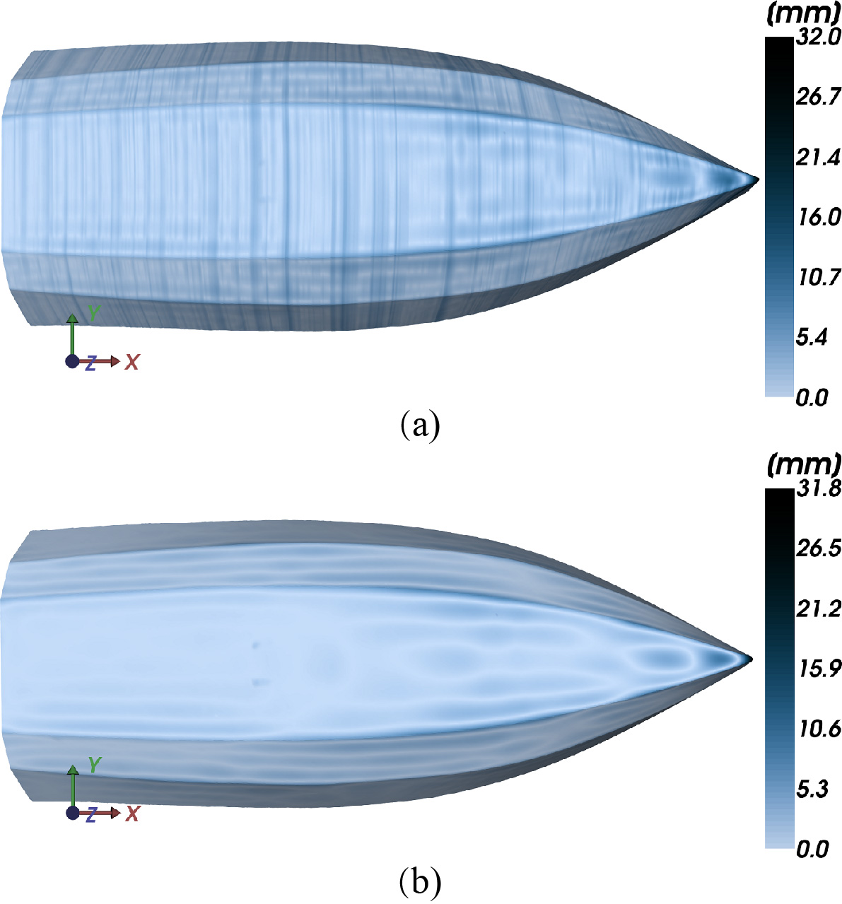

It follows directly from the definition of the error functions that the error defined by the minimization function Eq. 15 is larger or equal than the actual fitting error Eq. 11, as clearly confirmed by Fig. 7.

Once the initial linear fitting has been accomplished, the procedure developed in this paper proceeds from the respective ‘linear’ solution treating it as the initial solution for the subsequent non-linear fitting. More specifically, the proposed procedure applies the nonlinear gradient method Levenberg-Marquardt for the follow-up minimization of the fitting error, now treating all of $\bm{u},\bm{v},\bm{Q}$ and ${\bm{W}}$ as optimization variables. In each step of the proposed procedure a system of equations employing the Jacobi matrix ${\bm{J}}$ is solved, portions of which are formulated by partial differentiation according to Eq. 15,

$\displaystyle{\bm{J}}_{{\bm{u}}}=\frac{\partial{\bm{E}}}{\partial{\bm{u}}}\in{% \mathbb{R}}^{3\left(m_{0}+1\right){(m}_{1}+1)\times(m_{0}+1)},$ $\displaystyle{\bm{J}}_{{\bm{v}}}=\frac{\partial{\bm{E}}}{\partial{\bm{v}}}\in{% \mathbb{R}}^{3\left(m_{0}+1\right){(m}_{1}+1)\times(m_{1}+1)},$ (16) $\displaystyle{\bm{J}}_{{\bm{Q}}}=\frac{\partial{\bm{E}}}{\partial{\bm{Q}}}\in{% \mathbb{R}}^{3{\left(m_{0}+1\right){(m}_{1}+1)\times 3(n}_{0}+1)(n_{1}+1)},$ $\displaystyle{\bm{J}}_{{\bm{w}}}=\frac{\partial{\bm{E}}}{\partial{\bm{W}}}\in{% \mathbb{R}}^{3{\left(m_{0}+1\right){(m}_{1}+1)\times(n}_{0}+1)(n_{1}+1)}.$

The overall Jacobi matrix takes the form ${\bm{J}}=[{\bm{J}}_{{\bm{u}}}$ ${{\bm{J}}}_{{\bm{v}}}{{\bm{J}}}_{{\bm{Q}}}{{\bm{J}}}_{{\bm{W}}}]$ .

Figure 8(a) displays the resulting new values of the ${\bm{U}}$ and ${\bm{V}}$ matrices while Fig. 8(b) presents the entire solution of the proposed Levenberg-Marquardt fitting with respect to the degrees of freedom consisting of $\bm{u},\bm{v},\bm{Q}∼{}{i}∼{}{\bm{W}}$ .

Figure 8.

Result of Levenberg-Marquardt based non-linear fitting using Eq. 16. (a) Matrices 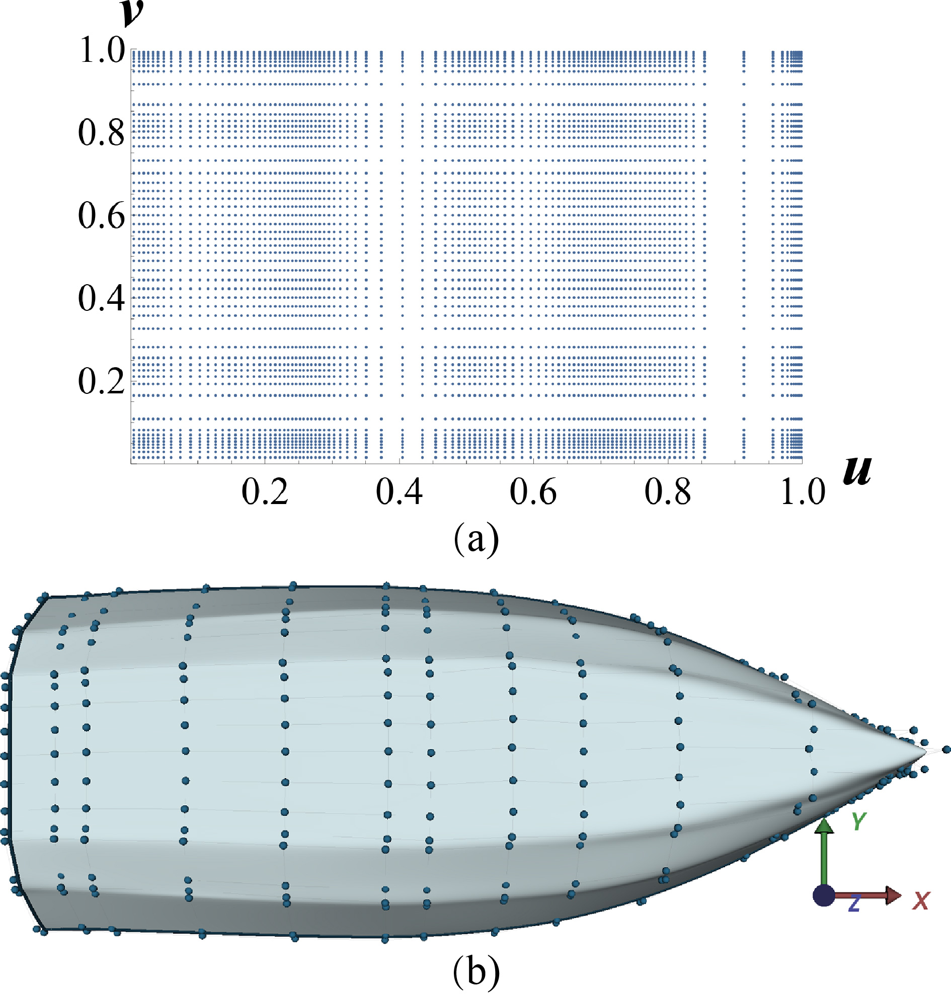${\bm{U}}$ and ${\bm{V}}$ ; (b) NURBS surface.

It can be clearly observed in Fig. 8(b) that the control points heap up and concentrate in areas with significant change of geometry. This enables the fitted surface to be numerically superior and adhere better to the given geometry ${\bm{P}}$ . This is the primary outcome of the optimization procedure. As all coordinates of the control points in ${\bm{Q}}$ are optimization variables, error minimization has pushed them towards the edges since such a distribution of ${\bm{Q}}$ led to the minimum possible error norm. Figure 8(a) shows the associated opposite effect of the developed fitting procedure on the rows and columns in the ${\bm{U}}$ and ${\bm{V}}$ matrices which tend to become less crowded with a somewhat diluted density around the edges.

This effect can be explained by recalling the fact that with NURBS surfaces a change of a control point ${\bm{Q}}_{i_{0}i_{1}}$ only affects the surface within the subdomain given by the knots $[\bar{u}_{i_{0}},\bar{u}_{i_{0}+d_{0}+1}\rangle\times[\bar{v}_{i_{1}},\bar{v}_% {i_{1}+d_{1}+1}\rangle$ . For the points ${\bm{P}}_{j_{0}j_{1}}$ of the matrix ${\bm{P}}$ , the assumption Eq. 8 stated that ${{\bm{C}}(u}_{j_{0}j_{1}},v_{j_{0}j_{1}})={\bm{P}}_{j_{0}j_{1}}$ , whereby $u_{j_{0}j_{1}}\in[\bar{u}_{i_{0}},\bar{u}_{i_{0}+d_{0}+1}\rangle$ and $v_{j_{0}j_{1}}\in[\bar{v}_{i_{1}},\bar{v}_{i_{1}+d_{1}+1}\rangle$ . If more neighboring control points are to be ‘encouraged’ to be located in the edge zone, then more neighboring knot-defined intervals should be embraced. Figure 9 demonstrates this effect in one dimension. These arguments provide some insight into the resulting distribution in Fig. 8(a).

Figure 9.

Conceptual illustration in 1D: impact of the developed non-linear fitting procedure, larger points ( ${\bm{Q}}_{i}$ ) denote control points, smaller points denote geometry (column of the matrix ${\bm{P}}$ ), $\bar{u}$ values denote the knot set like in Eq. 3 for degree $p=2$ , and arrows denote the associated parametric value $u_{i}$ for each point of the geometry. The relocation of the control points in Fig. 9(b) is a consequence of the relocation of the $u_{i}$ parameter values of the points of the geometry imposed by Eqs 15 and 16. (a) Almost equidistant arrows (parametric values $u_{i}$ ) indicate equidistant positions of the associated control points in curvilinear coordinates; (b) Less dense arrows (parametric values $u_{i}$ ) indicate more dense positions of the associated control points in curvilinear coordinates.

In order to achieve increased density of the control points ${\bm{Q}}_{3},{\bm{Q}}_{4}$ and ${\bm{Q}}_{5}$ in the area of the geometric feature and conseqently a better global solution (Fig. 9(b)), the proposed numerical approach disperses the parametric values of the associated points of the geometry to the whole domain where ${\bm{Q}}_{3},{\bm{Q}}_{4}$ and ${\bm{Q}}_{5}$ have impact. The small points in the neighborhood of those three control points represent the geometric feature. In the case where the parametric values $u_{i}$ are almost equidistant (Fig. 9(a)), all control points are equally employed which results in equidistant positions of the control points in curvilinear coordinates.

The fitting error of the non-linear fitting procedure based on the Levenberg-Marquardt method as described above is visualized in Fig. 10.

Figure 10.

Error generated by Levenberg-Marquardt based non-linear fitting, Eqs 15 and 16. (a) Deviation according to minimization function; (b) Deviation with respect to the closest point on the surface (actual geometric error).

Again, the error in Fig. 10(a) is based on the definition in Eq. 15, and the error in Fig. 10(b) is the actual fitting error Eq. 11.

The cumulation of the control points in areas with significant change of shape accomplished by the developed procedure has resulted in the important achievement of reducing the fitting error in those areas, an effect also demonstrated in [36]. This is illustrated in Fig. 11 which visualizes the difference in the respective fitting error between the linear fitting procedure (Fig. 7(a)) and the proposed enhanced non-linear procedure (Fig. 10(a)).

Figure 11.

Difference of fitting error generated by linear- and Levenberg-Marquardt based non-linear fitting.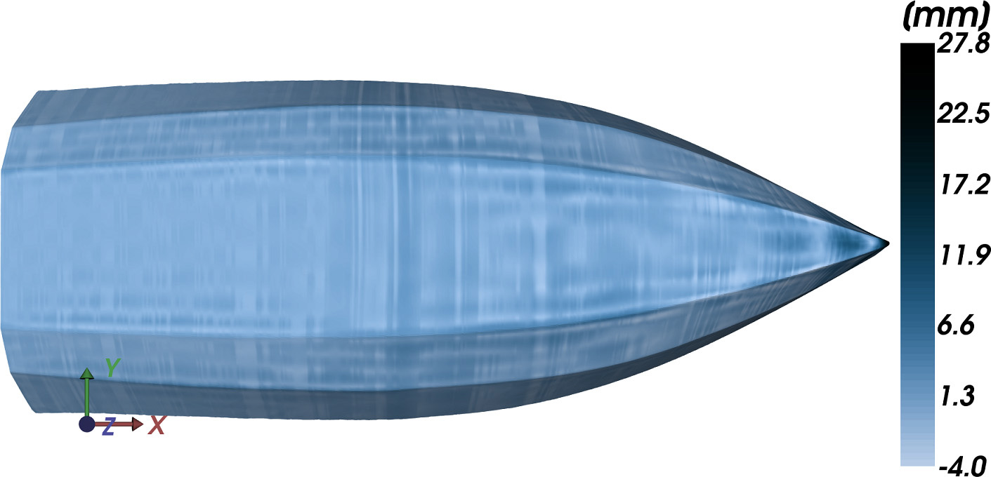

4.5 Some numerical difficulties of enhanced best-fitting

While offering major improvements in performance, the proposed procedure with the augmented vector of degrees of freedom ${\bm{u}}$ , ${\bm{v}}$ , ${\bm{Q}}$ and ${\bm{W}}$ for best-fitting does not come without some numerical drawbacks. Obviously, higher numerical complexity of gradient-based non-linear fitting instead of a simple linear procedure is one, the increased number of variables in ${\bm{u}}$ , ${\bm{v}}$ , ${\bm{Q}}$ and ${\bm{W}}$ is another.

However, a significant problem which may occur is geometric singularity, Fig. 12, which may be caused by several reasons. Geometric singularity may be the consequence of losing the device $u_{0}\leqslant u_{1}\leqslant\ldots\leqslant u_{m_{0}}$ or $v_{0}\leqslant v_{1}\leqslant\ldots\leqslant v_{m_{1}}$ in terms of the corresponding monotonously ordered sequences. Another related cause of singularity is the heaping of the parameters in ${\bm{U}}$ and ${\bm{V}}$ and their cumulation at some values.

Geometric singularity with this regard is a local optimum which cannot be escaped easily. At the edge of the singularity, the normals of the surface deviate from the normals of the given geometry, Fig. 12(c). A suitable intervention to avoid singularity is to augment the error norm in Eq. 15 by additional terms quantifying the difference of the corresponding normals in the given geometry and those of the fitted surface.

Figure 12.

Example of geometric singularity, (a) Geometry, (b) NURBS surface as the solution of the linear fitting problem, (c) NURBS surface as the solution of Levenberg-Marquardt based non-linear fitting.

Figure 13.

A test example for the gradient-based non-linear fitting. (a) Formula-student racing car; (b) Geometry.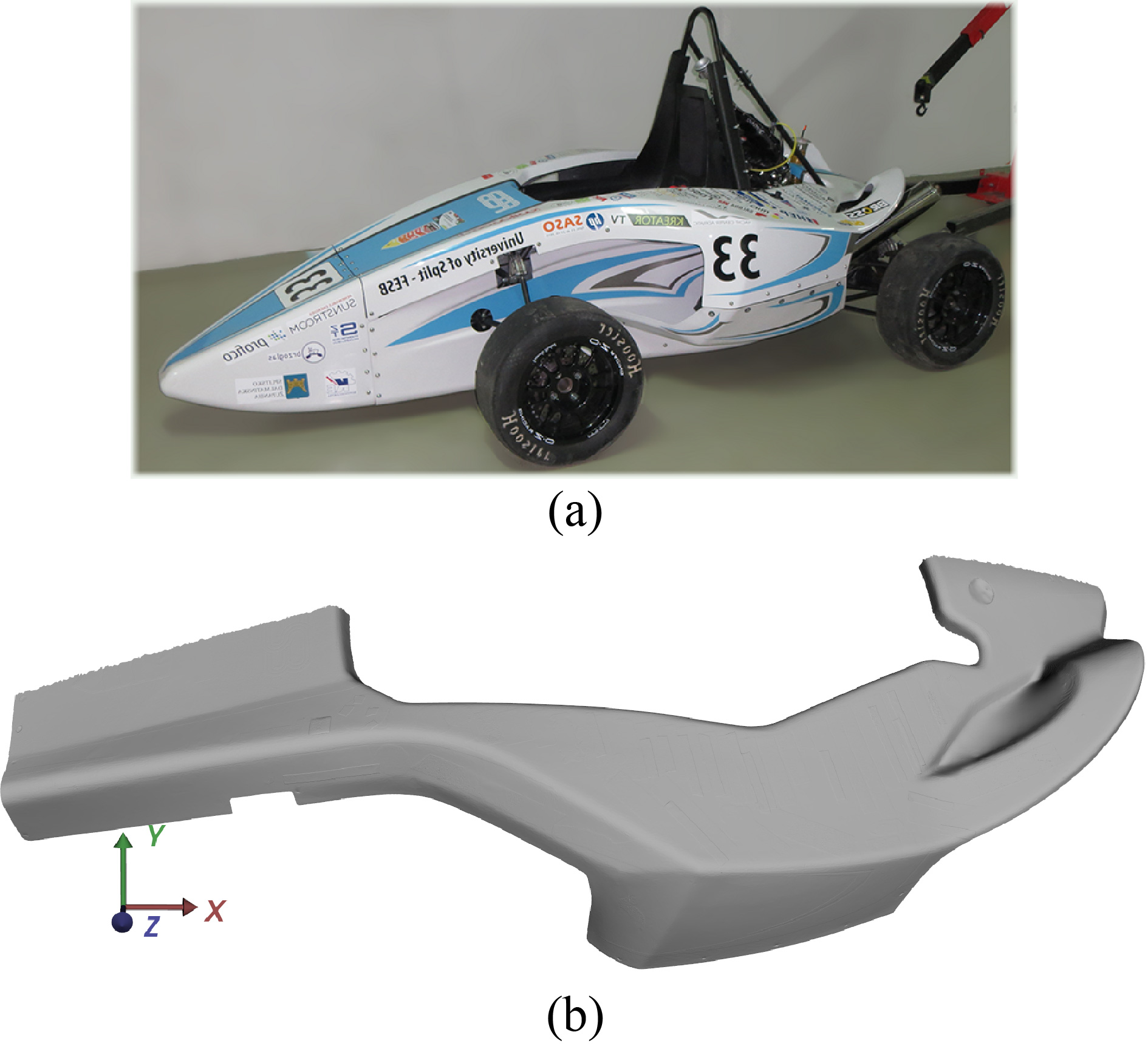

Another numerical difficulty which may potentially arise is related to the intervals of the parameter values which should be contained within the ranges given by $0=u_{0}\leqslant u_{1}\leqslant\ldots\leqslant u_{m_{0}}=1$ and $0=v_{0}\leqslant v_{1}\leqslant\ldots\leqslant v_{m_{1}}=1$ . During the course of the proposed best-fitting procedure with regard to the optimization variables given by ${\bm{u}}$ , ${\bm{v}}$ , ${\bm{Q}}$ and ${\bm{W}}$ , the ranges of values $[u_{0},u_{m_{0}}]=[0,1]$ and $[v_{0},v_{m_{1}}]=[0,1]$ may get scaled. This situation is displayed in Figs 14(a) and (b), where during the Levenberg-Marquardt error minimization with respect to u , ${\bm{v}}$ , ${\bm{Q}}$ and ${\bm{W}}$ , the respective ranges were modified to $[u_{0},u_{m_{0}}]=[0.024;$ $0.999]$ and $[v_{0},v_{m_{1}}]=[0.029;$ $0.98]$ in the case of Fig. 14(a) and $[u_{0},u_{m_{0}}]=[0.008;$ $1.221]$ and $[v_{0},v_{m_{1}}]=[0.037;$ $0.994]$ in the case of Fig. 14(b). This undesired scaling of the ranges of parametric values does not jeopardize the modeling or shape representation provided by the NURBS surface. A problem may however arise if multiple NURBS surfaces are to be chained into a single (piecewise) one, since common procedures of joining surfaces require that the last row/column of control points of one surface coincides with the first row/column of the second surface’s control points. This effect is illustrated in Fig. 14 showing the parameterization of a formula-student body shell (Fig. 13). The effect results in the extra surface which exists in Figs 14(a) and (b) with respect to original geometry in Fig. 13(a).

The object in Fig. 13(a), digitized by virtue of optical 3D scanning into the cloud in Fig. 13(d). represents a complex test-shape for the proposed method. Two different sizes of the parameters set were applied, 30 $\times$ 15 CP (Figs 14(a), (c) and (e) and 15 $\times$ 10 CP Figs 14(b), (d) and (f)). Two error distributions are presented, based on minimization function (Figs 14(d) and (e)) and actual closest-point error (Figs 14(d) and (e)).

Figure 14.

The results of gradient-based non-linear fitting for Fig. 13, left side (a, c, e) using 30 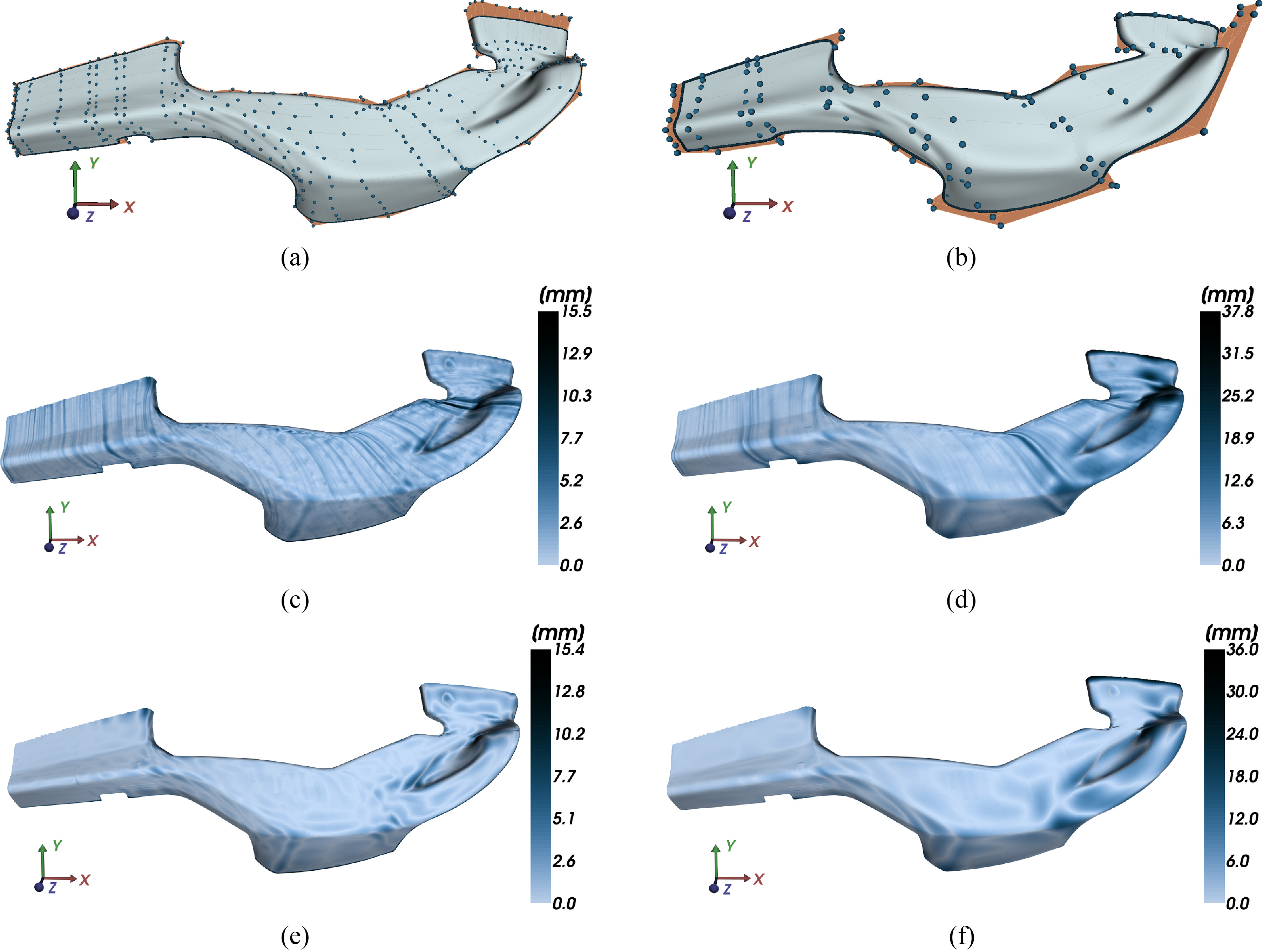$\times$ 15 control points, both degrees equal 3, right column (b, d, f) using 15 $\times$ 10 control points, both degrees equal 3. (a) NURBS surface, 30 $\times$ 15 CP; (b) NURBS surface, 15 $\times$ 10 CP; (c) Deviation according to minimization function, case in (a); (d) Deviation according to minimization function, case in (b); (e) Deviation with respect to closest point on the surface (actual geometric error), case in (a); (f) Deviation with respect to closest point on the surface (actual geometric error), case in (b).

Using more control points (Fig. 14) results in less error both according to the minimization function and also in terms of actual error (with respect to closest point). Regardless of respectively larger error, the right column example (case b) represents a numerically satisfactory solution in terms of dynamic parameterization, which confirms the quality of the proposed method. This confirms that the proposed non-linear fitting provides a satisfactory representation of the shape even for a moderate-sized set of fitting variables and that the error reduces further for a higher multitude of fitting parameters.

4.6 Enhanced best-fitting using external functions

The procedure developed in this paper builds a further enhancement on top of the improved result of non-linear fitting illustrated in Fig. 8(b) and based on error minimization as formulated in Eq. 15 with respect to ${\bm{Q}}$ and ${\bm{W}}$ in Eqs 4 and 5 and ${\bm{U}}$ and ${\bm{V}}$ according to Eqs 13 and 14. This further improvement is inspired by the fact that the non-linear fitting solution of Fig. 8(b) may still maintain more control points than necessary in monotonous areas without significant geometric features such as the mid-sections of the sailing boat hull. Due to symmetry of the parameter values (equal rows/columns in Eqs 13 and 14), the developed non-linear fitting as presented up to this point by itself did not reduce the number of control points in monotonous zones.

The solution of the Levenberg-Marquardt non-linear best fitting procedure (LM) as elaborated so far and displayed in Fig. 8(a) is now taken as the initial solution for the matrices ${\bm{C}}^{u}$ and ${\bm{C}}^{v}\in\mathbb{R}^{(m_{0}+1)\times(m_{1}+1)}$ in the next best-fitting stage, Eqs 13 and 14. In the next stage, the objective is to reduce the number of ‘surplus’ points in the areas external to zones of any significant geometric features. Smooth external functions will be engaged to execute such a change, and the optimization itself will be executed by genetic algorithms (GA) acting on the degrees of freedom of the external functions. As already stated, separate changes of individual elements which are not accompanied by corresponding changes of their surroundings may lead to singularity. Therefore, correspondingly smooth external functions must be applied. A basic GA algorithm was applied with few generations, whereby a physically reasonable initial population adequate for the given geometry was submitted. This elementary approach was shown to be sufficient. No further evaluations of different GA setups was conducted at this point.

In this paper, the function to implement the change in the matrices ${\bm{C}}^{u}$ and ${\bm{C}}^{v}$ in Eqs 13 and 14 controlled by the genetic algorithm optimizer for given parameters $\sigma_{u},\sigma_{v}\in\mathbb{R}$ and the pair $(c_{u},c_{v})\in\mathbb{R}^{2}$ is selected to be

$\displaystyle\begin{bmatrix}c_{j_{0}j_{1}}^{u}\\ c_{j_{0}j_{1}}^{v}\\ \end{bmatrix}^{\textit{NEW}}={\bm{\chi}}^{\textit{GA}}\left(\begin{bmatrix}c_{% j_{0}j_{1}}^{u}\\ c_{j_{0}j_{1}}^{v}\\ \end{bmatrix}^{\textit{OLD}}\right)$ $\displaystyle=\begin{bmatrix}c_{j_{0}j_{1}}^{u}\\ c_{j_{0}j_{1}}^{v}\\ \end{bmatrix}^{\textit{OLD}}+\begin{bmatrix}\left(c_{u}-c_{j_{0}j_{1}}^{u}% \right)\exp(-\sigma_{u}\left\|\Delta\right\|)\\ \left(c_{v}-c_{j_{0}j_{1}}^{v}\right)\exp(-\sigma_{v}\left\|\Delta\right\|)\\ \end{bmatrix},$ (17)

with $\Delta=\begin{bmatrix}c_{j_{0}j_{1}}^{u}-c_{u}\\ c_{j_{0}j_{1}}^{v}-c_{v}\\ \end{bmatrix}$ .

The parameters exposed to the genetic algorithm are $\sigma_{u}$ and $\sigma_{v}$ which control the width of the change and the pair $(c_{u},c_{v})$ which control the center of the change. Instead of our choice of the function ${\bm{\chi}}^{\textit{GA}}$ , it could also be any other smooth function that generates the increased density in the specified area. Figures 16(a) and (b) visualize the impact of the function $\bm{\chi}^{\textit{GA}}$ in Eq. 17 on the matrices ${\bm{C}}^{u}$ and ${\bm{C}}^{v}$ in Eqs 13 and 14 after the Levenberg-Marquardt procedure had been executed. Figures 16(a) and (b) demonstrate the success of the approach. Changing the values of the ${\bm{C}}^{u}$ and ${\bm{C}}^{v}$ matrices by applying external functions is expected to result in loss of symmetry of the parameter values, i.e. unequal values of rows/columns in Eqs 13 and 14. As a result, the distribution of the control points will also be asymmetric.

4.7 Building the external function

In the following text, ‘LMRC’ will refer to applying the Levenberg-Marquardt non-linear fitting with respect to the rows and columns ${\bm{u}}$ and ${\bm{v}}$ and ‘GAEF’ to applying genetic-algorithm-based optimization of external function parameters.

Figure 15 shows the distribution of the function

$f_{1}(T\in\mathbb{R}^{3})=\frac{\min\left\{\lambda_{1}^{T},\lambda_{2}^{T},% \lambda_{3}^{T}\right\}}{\lambda_{1}^{T}+\lambda_{2}^{T}+\lambda_{3}^{T}}$ (18)

which assigns the value of the eigenvalue ( $\lambda_{i}^{T}$ ) ratio of the covariance matrix of a local subset of a point cloud in the local neighborhood of ${\bm{T}}$ to each point ${\bm{T}}$ of the 3D cloud and hence also to the matrix ${\bm{P}}$ . This ratio is related to the complexity of the local geometry in the neighborhood of a point. The expression in Eq. 18 can be efficiently applied to detect features in the 3D data-points set as explained next.

In the cases when one of the eigenvalues is significantly smaller than the other two which are almost equal ( $\lambda_{i}^{T}\ll\lambda_{j}^{T}\leqslant\lambda_{k}^{T}$ ), then the neighborhood of the point is close to a plane surface and the function $f_{1}$ tends to 0. In cases where the minimum eigenvalue is significantly smaller than the mid-eigenvalue and the latter is significantly smaller than the maximum eigenvalue ( $\lambda_{i}^{T}\ll\lambda_{j}^{T}\ll\lambda_{k}^{T}$ ), then the neighborhood of that point is an edge. In order for the surrounding of the point to be a peak, all three eigenvalues must be almost equal ( $\lambda_{i}^{T}\approx\lambda_{j}^{T}\approx\lambda_{k}^{T}$ ).

Combining the functions ${\bm{\chi}}^{\textit{GA}}$ and $f_{1}$ provides potential for accelerated fitting. In fact, the reciprocical values of the eigenvalue ratio can be employed as weight factors in changing the values of the ${\bm{C}}^{u}$ and ${\bm{C}}^{v}$ matrices. In areas with significant change of geometry there is limited likelyhood for change of the ${\bm{C}}^{u}$ and ${\bm{C}}^{v}$ matrices, whereas in monotoneous areas the likelyhood is higher. That means that we should apply the function $\bm{\chi}^{\textit{GA}}$ only to areas with small values of the function $f_{1}$ (Fig. 15).

This corresponds to the intention in this step of the procedure, namely less dense distribution of control points in monotoneous zones and their higher density in zones with intensive change of shape.

Figure 15.

Distribution of eigenvalue ratios for matrix 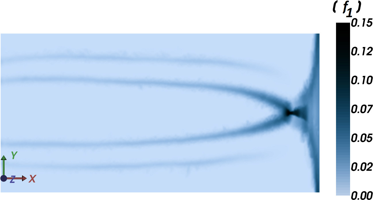${\bm{P}}$ .

Figure 16.

Result of genetic-algorithm based optimization with external functions (GAEF), 15 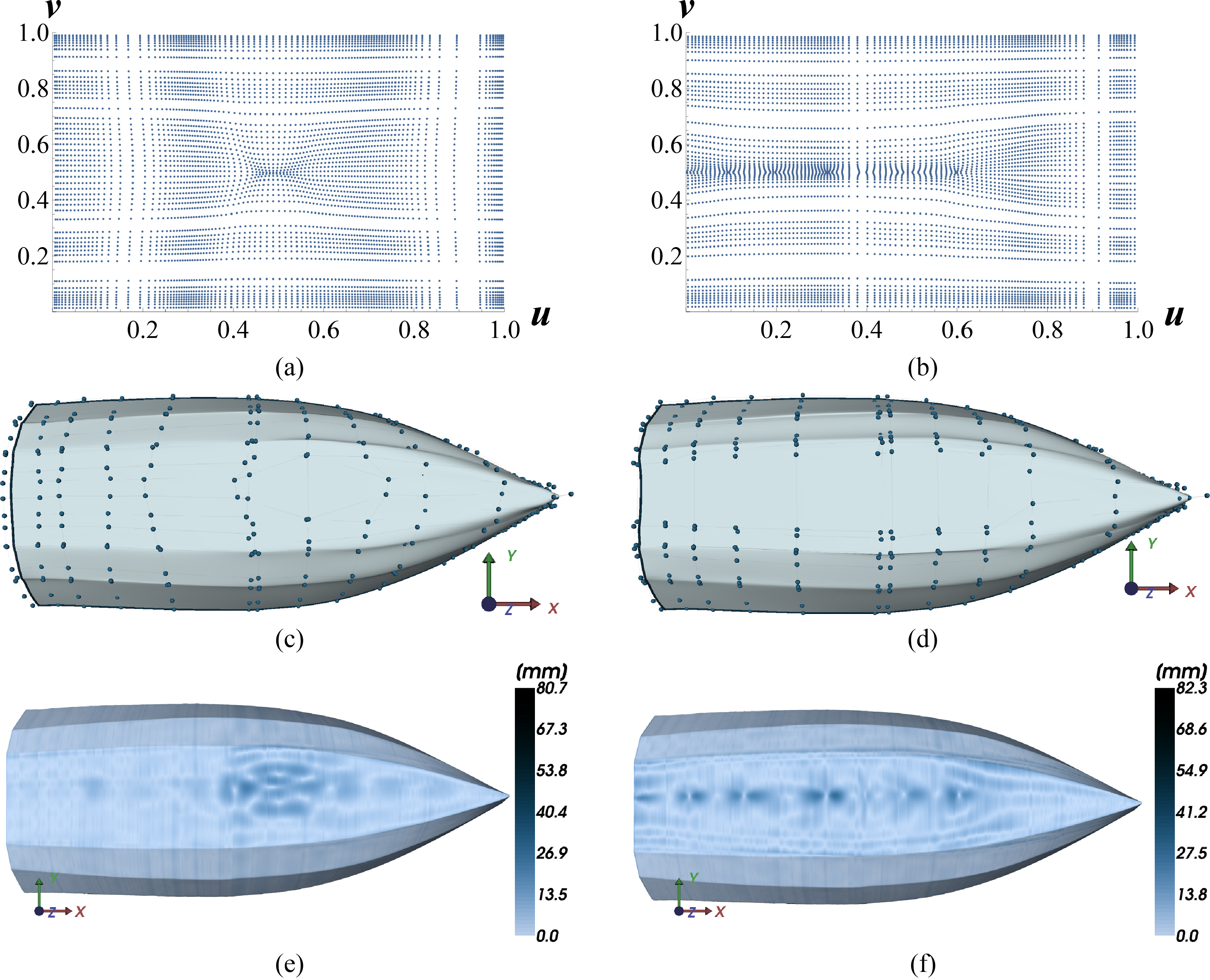$\times$ 20 control points, both degrees equal 3. Left column (a, c, e) shows results after one call of the function ${\bm{\chi}}^{\textit{GA}}$ with parameters: $c_{u}=c_{v}=0.5$ , $\sigma_{u}=\sigma_{v}=10$ . Right column (b, d, f) shows results after seven chained calls of the function ${\bm{\chi}}^{\textit{GA}}$ with parameters: $c_{u}=$ 0.0, 0.1, 0.2, 0.3, 0.4, 0.5, 0.6, $c_{v}=0.5$ , $\sigma_{u}=70$ , $\sigma_{v}=10$ . (a) Matrices ${\bm{U}}$ and ${\bm{V}}$ after GAEF, single ${\bm{\chi}}^{\textit{GA}}$ call; (b) Matrices ${\bm{U}}$ and ${\bm{V}}$ after GAEF, 7 ${\bm{\chi}}^{\textit{GA}}$ calls; (c) NURBS surface as solution of GAEF, single ${\bm{\chi}}^{\textit{GA}}$ call; (d) NURBS surface as the solution of GAEF, 7 ${\bm{\chi}}^{\textit{GA}}$ calls; (e) Fitting after GAEF, deviation according to minimization function, single ${\bm{\chi}}^{\textit{GA}}$ call; (f) Fitting after GAEF, deviation according to minimization function, 7 ${\bm{\chi}}^{\textit{GA}}$ calls.

4.8 Building the external function

As a summary, the nonlinear best fitting developed and demonstrated here consists of two subsequent procedures, the first being gradient-based fitting error minimization with respect to ${\bm{u}}$ , ${\bm{v}}$ , ${\bm{Q}}$ and ${\bm{W}}$ , (LMRC) and the second being non-gradient genetic algorithm based fitting error minimization with respect to the free parameters of an external function (GAEF), $\sigma_{u}$ , $\sigma_{v}$ , ${\bm{c}}_{u}$ , ${\bm{c}}_{v}$ . After both sub procedures have been applied consecutively, the matrices ${\bm{U}}$ and ${\bm{V}}$ are set to ${\bm{C}}^{u}$ and ${\bm{C}}^{v}$ respectively.

From the theoretical point of view it seems insignificant in which order the fitting error is minimized, by applying LMRC followed by GAEF or vice-versa. Numerical tests have shown that for objects with symmetric portions LMRC followed by GAEF may be the better option. Alternating application of LMRC and GAEF in the solution space makes the procedure swap from one local optimum to another. The symmetric solution produced by LMRC is converted to an asymmetric, improved solution by GAEF.

Already after the first GAEF execution, further iterations all yield asymmetric solutions. This is not an issue for the follow-up LMRC steps since the error function Eq. 15 does not require the rows/columns of the ${\bm{C}}^{u}$ and ${\bm{C}}^{v}$ to have the same values, i.e. they are only changed (moved) by the same values $u_{j_{0}}$ and $v_{j_{1}}$ . It can therefore be expected that minimization of the fitting error in one iteration causes aggregation of the control points in one zone, while the next iteration may cause their heaping up in another zone.

As a concluding remark related to the developed fitting procedure it should be stressed that the ultimate objective is to obtain a NURBS surface which represents the geometry of some object with required accuracy. The accuracy is measured by squared deviations such that good fitting can be obtained by least-squares formulations. Two different combinations of the steepest descent method and Newton’s method were applied, the Levenberg-Marquardt (LM) and Dog Leg (DL) methods. The algorithm is executed until the value of the deviation error function is reduced below the prescribed tolerance. Both methods use the corresponding Jacobian which is here approximated numerically, hence the number of degrees of freedom was reduced for computational efficiency. The LM method has produced the requested accuracy in all test cases and determined the resulting NURBS surface for all selections of the damping term.

Figure 17.

Automotive crankshaft as a test object, 25 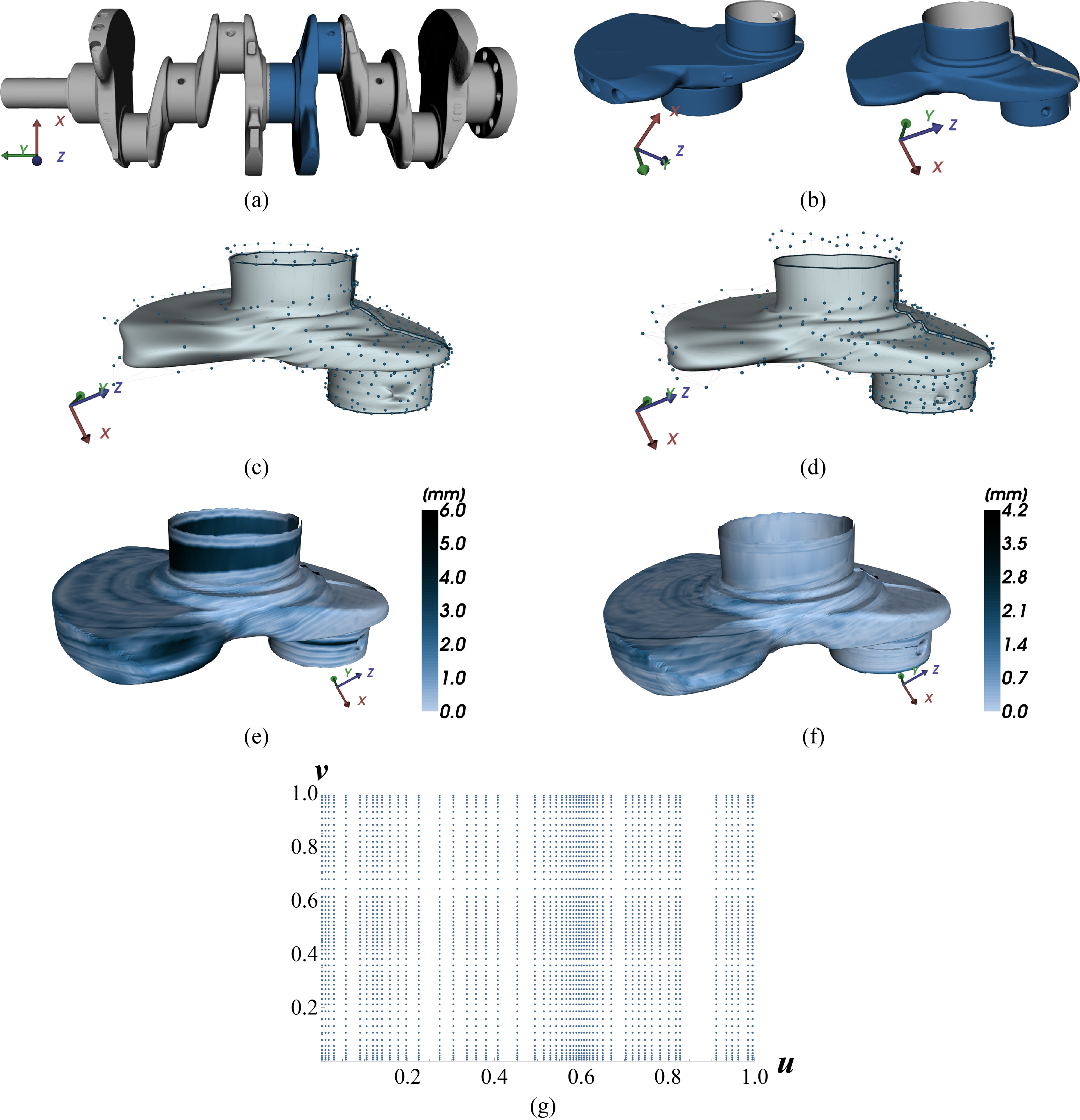$\times$ 25 control points, both degrees equal 3. (a) Geometry with a prominent part; (b) Part of the geometry-two views; (c) Fitting based on linear procedure (integral NURBS surface); (d) Fitting based on LMRC (integral NURBS surface); (e) Fitting based on linear procedure, deviation according to minimization function; (f) Fitting based on LMRC, deviation according to minimization function; (g) Matrices ${\bm{U}}$ and ${\bm{V}}$ after processing by LMRC.

Figure 18.

Result of genetic-algorithm based optimization with external functions (GAEF), 35 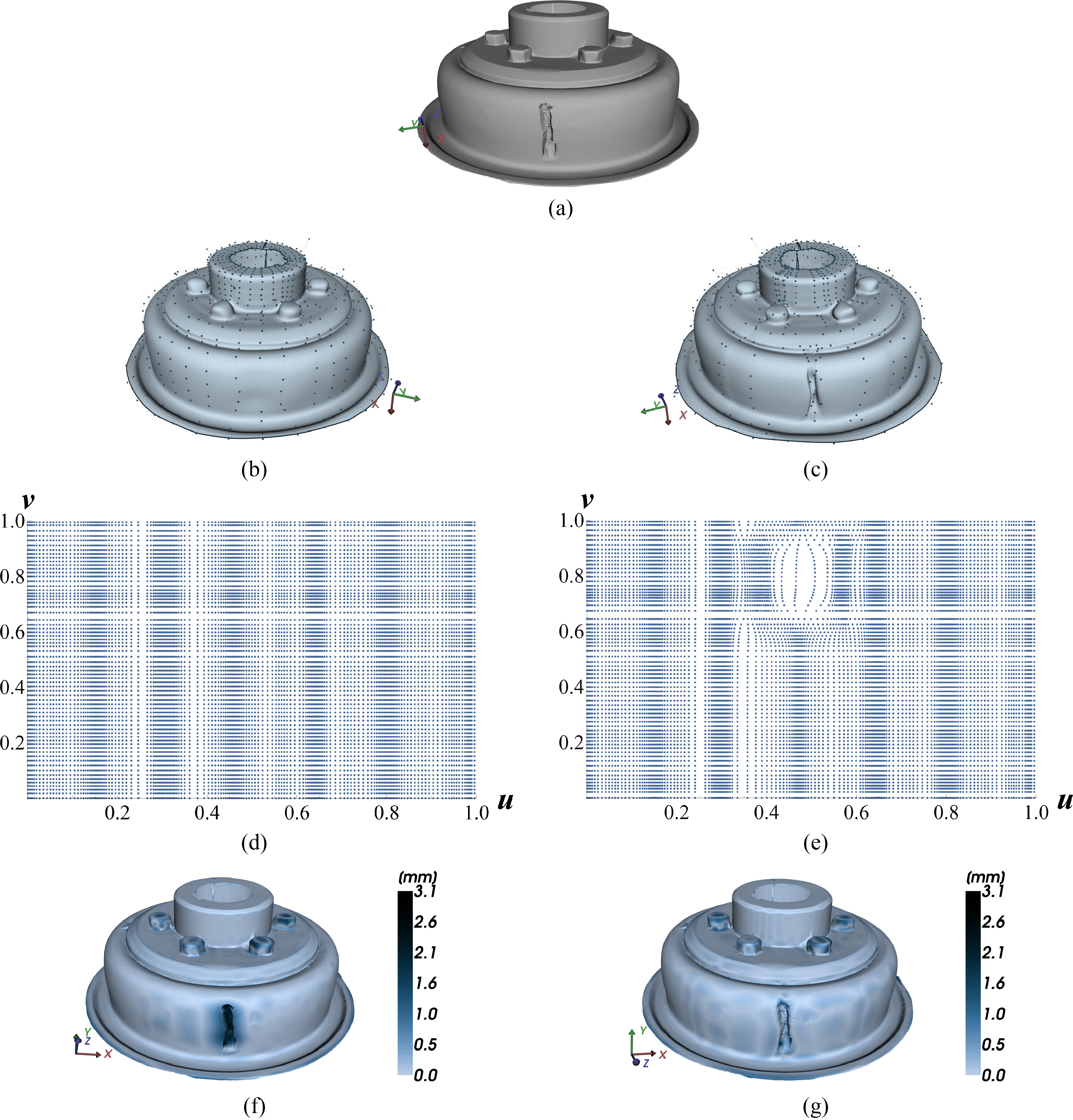$\times$ 30 control points, both degrees equal 3. Left column (b, d, f) shows LM results. Right column (c, e, g) shows results after seven chained calls of the function ${\bm{\chi}}^{GA}$ with parameters: $c_{u}=0.37,0.375,\ldots,0.39$ , $c_{v}=0.65,0.70,\ldots,0,95$ , $\sigma_{u}=80$ , $\sigma_{v}=500$ . (a) Geometry; (b) NURBS surface as the solution of LMRC; (c) NURBS surface as the solution of GAEF, 35 ${\bm{\chi}}^{\textit{GA}}$ calls; (d) Matrices ${\bm{U}}$ and ${\bm{V}}$ after processing by LMRC; (e) Matrices ${\bm{U}}$ and ${\bm{V}}$ after GAEF, 35 ${\bm{\chi}}^{\textit{GA}}$ calls; (f) Fitting based on LMRC, deviation according to minimization function; (g) Fitting after GAEF, deviation according to minimization function, 35 ${\bm{\chi}}^{\textit{GA}}$ calls.

On the other hand, the DL method has not produced good results. While better results were obtained for smaller trust regions, the error could not be significantly reduced any further after the few initial iterations and was still less precise than the LM result. Since the DL procedure requires fewer calculations of the Jacobi matrix, the DL was applied in cases with larger multitudes of degrees of freedom, nevertheless the execution failed in those cases. It can be assumed that the DL procedure cannot accomplish the required accuracy because of the many local minima of the function. While the LM method has the capacity of escaping neighborhoods of local optima even after a few iterations, the DL procedure cannot do it based on Newton’s iterations. Hence the conclusion here is that the LM method should be the method of choice for acquiring precise and robust solutions in NURBS surface fitting.

5. Test results, discussion and critical analysis

In the following, we provide examples that encompass a spectrum of engineering objects and demonstrate the robustness of the developed approach. We decided to test the performance of our method on real engineering objects rather than numerically generated surfaces since this is less biased, especially as real objects embed real geometric features. The examples include visual presentations of geometries with prominent parts, respective NURBS surfaces after linear fitting and LMRC, deviations according to the minimization function and also the corresponding matrices ${\bm{U}}$ and ${\bm{V}}$ after LMRC. In the linear fitting process the matrices ${\bm{U}}$ and ${\bm{V}}$ have (fixed) uniform distributions of points and they look like shown in Fig. 5.

As mentioned in the introduction, we applied a projection of the shape into a rectangular domain in order to obtain a matrix topology of the matrix ${\bm{P}}$ . This way we were able to encompass the whole geometry including the topology. This assures that changing the position of the control point ${\bm{Q}}_{i}$ of the NURBS surface only affects the belonging part of the geometry.

The following example (Fig. 17) is a part of an automotive crankshaft which presents an extremely demanding shape. The part includes edges, cylinders and small hemispheres involving strong asymmetry which is undesirable in the process of fitting because of a much larger number of control points needed to describe such a shape.

Figure 17(a) shows the polygonised point set obtained by optical 3D scanning and corresponding processing, part of which is selected to test the developed procedure (Fig. 17(b)). Figure 17(d) presents the resulting distribution of the control points after applying the LMRC non-linear fitting developed in this paper as opposed to the standard linear fitting from literature (Fig. 17(c)). Figure 17(f) shows the improved fitting error distribution of the developed procedure accompanied by the ‘reference’ error distribution of the ‘standard’ linear fitting (Fig. 17(e)). The major improvement derives from the fact that the control points were able to relocate towards the more expressed features of the object while ‘leaving’ the ‘simpler’ shape portions such as the almost planar elements. Nevertheless, the improved fitting is not so evident visually in this example since most of the relocated control points were attracted towards the small hole on the right bottom part of the object, which is essentially a local shape feature. It can also be observed that the edges of the shape are much better pronounced with the developed enhanced fitting procedure. Nevertheless, the following example (Fig. 18) is selected such that it contains a local damage feature which visually more clearly emphasizes the advantages of the proposed method. Figure 17(g) shows the resulting distribution of the parameter values which accompanies Figs 17(d) and (f).

From the deviation according to the minimization function it is obvious that LMRC procedure results in less deviation in cylindrical areas (Fig. 17(f)). That is mainly attributed to the weighting factors of the NURBS surface. From the layout of the control points it is evident that cylindrical areas need a smaller number of control points to be described with respect to the linear problem. This is just a confirmation of the mathematical background of the NURBS definition.

This example (Fig. 17) also visualizes that relatively small geometric features such as a hemisphere or a bolt also have a sharper geometric presentation with respect to the corresponding linear fitting. Nevertheless, the drawbacks of single-patch NURBS parameterization for accurate presentation of geometries which include relatively small geometric features are here obvious. Such areas require more rows/columns to be represented. During optimization, the small features move the control points away from the areas of larger geometric features. Strictly mathematically, small features imply a larger number of local solutions. The error function in such cases does not possess local solutions which would represent the larger features with better accuracy. However, small local features may not be significant within the context of dynamic parameterization.

Figure 18 presents another complex example of an engineering object containing several local features (e.g. bolts, local damage). Figures 18(e) and (c) clearly indicate the improvement of the fitted surface at the location of the damage accomplished by GAEF as opposed to only applying LMRC (Figs 18(d) and (f)).

A question might arise why we present topology optimization and fitting based on parametric values in areas containing features (e.g. edges) as advantages of the proposed method. We could namely apply several NURBS patches with those edges as borders. The answer is embedded in the fact that the process in dynamic parameterization is excessively complicated, especially the procedure of automatic/semi automatic partitioning of the geometry. Moreover, the proposed method can easily be applied to partitions with geometric features in multi-partition parameterizations.

Table 1
The computational cost for example in Fig. 18

	CPU time (s)	No. of LM
		iterations
Linear fitting	3	n/a
Enhanced fitting 200 $\times$ 200	40	17
Enhanced fitting 500 $\times$ 200	140	38

The overall proposed procedure is shown in Algorithm 1.

Algorithm 1. Enhanced 3D parameterization for integrated shape synthesis by fitting parameter values to point sets

Input:

•

Mesh obtained from 3D scanning system;

•

Dimensions of matrix ${\bm{P}}$ : $(m_{0}+1)\times(m_{1}+1)$ ;

•

Number of control points: $(n_{0}+1)\times(n_{1}+1)$ ;

•

Degrees of basic function: $p_{u}$ and $p_{v}$ ;

Output: NURBS surface ${\bm{C}}$ begin

Projecting input mesh into rectangular domain;

Generating matrix ${\bm{P}}$ and corresponding parametric

matrices ${\bm{U}}$ and ${\bm{V}}$ ;

Detecting geometric features;

Linear problem – initial surface ${\bm{C}}$ ;

LMRC – improved surface ${\bm{C}}$ ;

while nIteration $>0$

GAEF in adjacency of dominant geometric

features;

nIteration $\leftarrow$ nIteration $-$ 1;

end while

return ${\bm{C}}$ ;end

The above examples clearly demonstrate the advantages of the proposed method. In terms of computational time and numerical complexity, Table 1 provides adequate insight for the example in Fig. 18.

The size of the respective matrix ${\bm{P}}$ was 200 $\times$ 200 and 500 $\times$ 200, and the PC we used for the calculation has an Intel Dual-Core processor with 3.0 GHz and 8 GB of RAM.

6. Conclusions

Shape optimization is increasingly becoming a key ingredient in engineering design, whereby the focal problem is frequently efficient, trustworthy and accurate geometric modeling. In many cases, re-enginee- ring of shape towards optimality involves using some existing shape as the initial solution in numerical optimization.

Shape optimization in engineering should in many cases not operate directly on some CAD database defining the elementary geometric primitives as constituents of the engineering object. This approach would be inefficient in such cases as many insignificant geometric details would be dealt with. Moreover, many constraint relationships in the CAD model would have to be obeyed during the shape optimization process. In such cases, relatively simple shape representation using overall 3D parametric surfaces or few chained piecewise surfaces would be much more beneficial for overall efficiency of shape optimization. Nevertheless, this requires sparing parameterizations with an as-small-as-possible multitude of shape parameters, yet providing high quality of shape representation, which is a challenging problem in itself. The numerical procedure presented in this paper develops several original numerical interventions to empower efficient integral 3D representation of engineering objects.

The developed procedure incorporates innovative non-linear fitting of NURBS surfaces consisting of gradient-based fitting error minimization with respect to NURBS control points and row/column-wise optimization of NURBS parameter values for the given geometry. This is followed by genetic-algorithm based optimization of parameters of external functions steering a further mode of displacement of the parameter values for the given geometry. The developed procedures are shown to be successful using several complex engineering objects.

Specifically, the proposed methodology combines several numerical operations into a single-patch non-linear NURBS fitting procedure. They include the

(iii) (i)

Formulation of an augmented set of fitting variables, which involve the parameter values of data points in addition to the control points and weight factors,

(ii)

Structuring of the augmented set for reasonable dimensionality,

(iii)

Enhanced fitting by gradient-based minimization with respect to the augmented set,

(iv)

Evolutionary fitting by applying external functions.

The complex-shape engineering objects used as test cases clearly demonstrate the efficiency of the proposed methodology in producing high-quality single-patch NURBS representations of given point sets. The comparisons with the results in literature were conducted such that both standard fitting (literature) and our proposed enhanced best fitting were applied on the same selected engineering objects.

The examples in Figs 17 and 18 which represent engineering objects with complex 3D shapes demonstrate the superior performance of the developed methodology in terms of geometric error and especially representation quality in areas with intensive local change of shape. The significantly improved representation accuracy of the developed procedure justifies the increased numerical effort of non-linear fitting. Moreover, the procedure is dynamically adaptive and does not require ‘maintenance’ of the knot set layout as do T-splines for dynamically changing shapes. Parameters that could be used to additionally confirm the performance of the method can be based on the error norms for example as given in Figs 17 and 18, globally for the overall object or locally for critical zones.

Footnotes

Acknowledgments

This work was supported by the Croatian Science Foundation [grant number IP-2014-09-6130].

References

Böhm

Farin

Kahmann

. A survey of curve and surface methods in CAGD. Comput Aided Geom Des [Internet]. 1984 Jul; 1(1): 1-60. Available from: http://linkinghub.elsevier.com/retrieve/pii/0167839684900037.

Campbell

Flynn

. A survey of free-form object representation and recognition techniques. Comput Vis Image Underst [Internet]. 2001 Feb; 81(2): 166-210. Available from: http://linkinghub.elsevier.com/retrieve/pii/S1077314200908890.

Campomanes-Álvarez

Cordón

Damas

. Evolutionary multi-objective optimization for mesh simplification of 3D open models. Integr Comput Aided Eng. 2013; 20(4): 375-90.

Cyganek

Siebert

. An introduction to 3D computer vision techniques and algorithms [Internet]. An Introduction to 3D Computer Vision Techniques and Algorithms. Chichester, UK: John Wiley & Sons, Ltd; 2009; p. 1-7. Available from: https://doi-wiley-com.web.bisu.edu.cn/10.1002/9780470699720.ch1.

Ćurković

Vučina

. 3D shape acquisition and integral compact representation using optical scanning and enhanced shape parameterization. Adv Eng Informatics [Internet]. 2014 Apr; 28(2): 111-26. Available from: http://linkinghub.elsevier.com/retrieve/pii/S1474034614000032.

Deb

Goel

. Multi-objective evolutionary algorithms for engineering shape design. In: Evolutionary Optimization [Internet]. Boston: Kluwer Academic Publishers; 2000; p. 147-75. Available from: https://link-springer-com.web.bisu.edu.cn/10.1007/0-306-48041-7_6.

Dimitri

De Lorenzis

Scott

Wriggers

Taylor

Zavarise

. Isogeometric large deformation frictionless contact using T-splines. Comput Methods Appl Mech Eng [Internet]. 2014 Feb; 269: 394-414. Available from: http://linkinghub.elsevier.com/retrieve/pii/S0045782513002971.

Dimitri

De Lorenzis

Wriggers

Zavarise

. NURBS- and T-spline-based isogeometric cohesive zone modeling of interface debonding. Comput Mech [Internet]. 2014 Aug 20; 54(2): 369-88. Available from: https://link-springer-com.web.bisu.edu.cn/10.1007/s00466-014-0991-7.

Eberly

. Least-Squares Fitting of Data with B-Spline Curves [Internet]. 2010; Available from: http://www.geometrictools.com.

10.

Eberly

. Least-Squares Fitting of Data with B-Spline Surfaces [Internet]. 2010; Available from: http://www.geomet-rictools.com.

11.

Eck

Hoppe

. Automatic reconstruction of B-spline surfaces of arbitrary topological type. In: Proceedings of the 23rd Annual Conference on Computer Graphics and Interactive Techniques – SIGGRAPH ’96 [Internet]. New York, New York, USA: ACM Press; 1996; p. 325-34. Available from: http://portal.acm.org/citation.cfm?doid=237170.237271.

12.

Farin

. Curves and Surfaces for Computer Aided Geometric Design: A Practical Guide. San Francisco/London: Morgan Kaufmann Publishers/Academic Press; 2002.

13.

GmbH

. Metrology Systems [Internet]. 2012. Available from: http://www.gom.com/metrology-systems/system-overview/atos.html.

14.

Kociecki

Adeli

. Shape optimization of free-form steel space-frame roof structures with complex geometries using evolutionary computing. Eng Appl Artif Intell [Internet]. 2015 Feb 38; 168-82. Available from: http://linkinghub.elsevier.com/retrieve/pii/S0952197614002528.

15.

Kruth

J-P

Kerstens

. Reverse engineering modelling of free-form surfaces from point clouds subject to boundary conditions. J Mater Process Technol [Internet]. 1998 Apr; 76(1–3): 120-7. Available from: http://linkinghub.elsevier.com/retrieve/pii/S0924013697003415.

16.

Cai

Zhang

Chen

. A method for topological entity matching in the integration of heterogeneous CAD systems. Integr Comput Aided Eng. 2013; 20(1): 15-30.

17.

Scott

. Analysis-suitable T-splines: Characterization, refineability, and approximation. Math Model Methods Appl Sci [Internet]. 2014 Jun; 24(6): 1141-64. Available from: https://www-worldscientific-com.web.bisu.edu.cn/doi/abs/10.1142/S0218202513500796.

18.

Kruth

J-P

. NURBS curve and surface fitting for reverse engineering. Int J Adv Manuf Technol [Internet]. 1998 Dec; 14(12): 918-27. Available from: https://link-springer-com.web.bisu.edu.cn/10.1007/BF01179082.

19.

Mencl

Muller

. Interpolation and approximation of surfaces from threedimensional scattered data points. In: Proceedings of Eurographics 98 Lisabon; 1998; p. 223-233.

20.

Meraoumia

Chitroub

Bouridane

. 2D and 3D palmprint information, PCA and HMM for an improved person recognition performance. Integr Comput Aided Eng. 2013; 20(3): 303-19.

21.

Nguyen

Kerfriden

Brino

Bordas

SPA

Bonisoli

. Nitsche’s method for two and three dimensional NURBS patch coupling. Comput Mech [Internet]. 2014 Jun 5; 53(6): 1163-82. Available from: https://link-springer-com.web.bisu.edu.cn/10.1007/s00466-013-0955-3.

22.

Peng

Gupta

. Model and algorithms for point cloud construction using digital projection patterns. J Comput Inf Sci Eng [Internet]. 2007; 7(4): 372. Available from: http://computingengineering.asmedigitalcollection.asme.org/article.aspx?articleid=1400963.

23.

Piegl

Tiller

. Parametrization for surface fitting in reverse engineering. Comput Des [Internet]. 2001 Jul; 33(8): 593-603. Available from: http://linkinghub.elsevier.com/retrieve/pii/S0010448500001032.

24.

Rao

. Engineering Optimization [Internet]. Hoboken, NJ, USA: John Wiley & Sons, Inc.; 2009. Available from: https://doi-wiley-com.web.bisu.edu.cn/10.1002/9780470549124.

25.

Riffnaller-Schiefer

Augsdörfer

Fellner

. Isogeometric shell analysis with NURBS compatible subdivision surfaces. Appl Math Comput [Internet]. 2016 Jan; 272: 139-47. Available from: http://linkinghub.elsevier.com/retrieve/pii/S0096300315008942.

26.

Rogers

Adams

. Mathematical Elements for Computer Graphics. New York: McGraw-Hill; 1989.

27.

Saitou

Izui

Nishiwaki

Papalambros

. A survey of structural optimization in mechanical product development. J Comput Inf Sci Eng [Internet]. 2005; 5(3): 214. Available from: http://computingengineering.asmedigitalcollection. asme.org/article.aspx?articleid=1400271.

28.

Samareh

. A survey of shape parameterization techniques. In: CEAS/AIAA/ICASE/NASA Langley International Forum on Aeroelasticity and Structural Dynamics, NASA/CP-1999-209136. 1999; p. 1; 333-344.

29.

Saridakis

Dentsoras

. Soft computing in engineering design – A review. Adv Eng Informatics [Internet]. 2008 Apr; 22(2): 202-21. Available from: http://linkinghub.elsevier.com/retrieve/pii/S1474034607000717.

30.

Sarkar

Menq

C-H

. Smooth-surface approximation and reverse engineering. Comput Des [Internet]. 1991 Nov; 23(9): 623-8. Available from: http://linkinghub.elsevier.com/retrieve/pii/001044859190038X.

31.

Sarma

Adeli

. Life-cycle cost optimization of steel structures. Int J Numer Methods Eng [Internet]. 2002 Dec 30; 55(12): 1451-62. Available from: https://doi-wiley-com.web.bisu.edu.cn/10.1002/nme.549.

32.

Sarma

Adeli

. Data parallel fuzzy genetic algorithms for cost optimization of steel structures. Int J Sp Struct. 2003; 18(3): 195-205.

33.

Seiffert

Khoshgoftaar

Van Hulse

. Hybrid sampling for imbalanced data. Integr Comput Aided Eng. 2009; 16(3): 193-210.

34.

Shah

Mantyla

. Parametric and feature-based CAD/CAM. New York: John Wiley & Sons, Ltd; 1995.

35.

Vucina

Lozina

Pehnec

. Computational procedure for optimum shape design based on chained Bezier surfaces parameterization. Eng Appl Artif Intell [Internet]. 2012 Apr; 25(3): 648-67. Available from: http://linkinghub.elsevier.com/retrieve/pii/S0952197611002181.

36.

Vučina

Ćurković

Novković

. Classification of 3D shape deviation using feature recognition operating on parameterization control points. Comput Ind [Internet]. 2014 Aug; 65(6): 1018-31. Available from: http://linkinghub.elsevier.com/retrieve/pii/S0166361514000797.

37.

Zhang

Han

. Quantitative optimization of interoperability during feature-based data exchange. Integr Comput Aided Eng [Internet]. 2015 Dec 8; 23(1): 31-50. Available from: http://www.medra.org/servlet/aliasResolver?alias=iospress&doi=10.3233/ICA-150499.

Enhanced 3D parameterization for integrated shape synthesis by fitting parameter values to point sets

Abstract

Keywords

1. Introduction

1.1 Background, rationale and objectives

2. Development of an efficient parameterization

4.1 Background

Table 1 The computational cost for example in Fig. 18

Footnotes

Acknowledgments

References

Table 1
The computational cost for example in Fig. 18