Quantum inspired evolutionary algorithms with improved rotation gates for real-coded synthetic and real world optimization problems

Abstract

We investigate two modified Quantum Evolutionary methods for solving real value problems. The Quantum Inspired Evolutionary Algorithms (QIEA) were originally used for solving binary encoded problems and their signature features follow superposition of multiple states on a quantum bit and a rotation gate. In order to apply this paradigm to real value problems, we propose two quantum methods Half Significant Bit (HSB) and Stepwise Real QEA (SRQEA), developed using binary and real encoding respectively, while keeping close to the original quantum computing metaphor. We evaluate our approaches against sets of multimodal mathematical test functions and real world problems, using five performance metrics and include comparisons to published results. We report the issues encountered while implementing some of the published real QIEA techniques. Our methods focus on introducing and implementing new rotation gate operators used for evolution, including a novel mechanism for preventing premature convergence in the binary algorithm. The applied performance metrics show superior results for our quantum methods on most of the test problems (especially for the more complex and challenging ones), demonstrating faster convergence and accuracy.

Keywords

Quantum evolutionary methods estimation of distribution algorithms performance metrics global optimization multimodal functions real value problems

1. Introduction

A challenge for modern computer science is the development of algorithms for increasingly complex optimisation problems. These may include a variety of practical real-world problems, such as structural engineering [24, 25], 3D mesh simplification [4], antenna design [7], wireless network design [34], electric power systems [1], resource allocation [27], digital image watermarking [42], EEG classification [21], benchmark problems [11], large data set analysis [31], or mathematical functions designed to test or challenge aspects of optimisation [22, 50]. Approaches to solving these problems include typical algorithms such as particle swarm optimisation (PSO) [36, 51], genetic algorithms (GA) [14, 39], and differential evolution [12, 23, 44], as well as other nature inspired methods such as honey bee [28] and cloud drops algorithms [9]. For a discussion of modern state of the art techniques, including memetic and landscape analysis techniques, see [6, 40, 56].

In 2002 a new optimization algorithm was presented in [18], that took inspiration from quantum computing to evolve a probability distribution, which in turn was employed to search a solution space. The method used a string of quantum bits (Qbit), each storing sampling probability of a one or a zero. Successive sampling of the string produced a series of candidate binary solutions. If any of these were found to be an improvement, the underlying Qbit probabilities were adjusted to make the candidate more likely to appear in successive samples. A detailed explanation of the algorithm is presented in Section 2.

Originally, this quantum-inspired evolutionary algorithm (QIEA) was applied to the Knapsack problem – a binary combinatorial optimisation problem [18], and then modified versions were applied by others to OneMax, Noisy-flat and NK-landscapes [35], neural-network training [45], and networking [49].

Although some attempts have been made to apply binary QIEA (bQIEA) to real-value problems [19], most applications to such tasks have used real-value QIEA (rQIEA) [3, 8, 20, 48, 54]. These algorithms took, at least superficially, the concepts of superposition and quantum rotation gates that were introduced with the binary QIEA, and adopted them for application to real-value problems. However, when reviewing them we encountered a number of problems. Many were incompletely described and could therefore not be reproduced, one was trivial to implement [54] but performed extremely badly on a set of multimodal mathematical test functions, and of greatest concern, one paper [8], which claimed superior performance to another optimization algorithm, but was later found to not have performed as well as claimed [43]. A second issue, more of a philosophical concern than a practical problem, is that in making the adaptation to real-value problems, the purity of the original quantum inspiration (that are naturally applied to binary problems) may be lost. We discuss these concerns in Sections 3 and 6. Various attempts at a real QIEA can be found in the literature, including [3, 20, 48], and in [53] a review is presented of both binary and real QIEA. In this investigation we have chosen [55] to build a real-coded QIEA upon, as it performed the best in initial tests and contained features common to many real QIEA.

The goals of the research presented here were to see how the Classic version [18] of the binary QIEA, as well as a representative real QIEA, would perform on a number of recent benchmark test functions and several real-world problems, and to investigate, design, and develop modified binary and real QIEA, proposed to improve the performance of these approaches in terms of convergence and accuracy. The bQIEA were shown to belong to a class of methods called estimation of distribution algorithms [35]. This work therefore extends the application of this class.

In our previous work [47], we presented an initial investigation of the binary QIEA. In the current paper we extend the investigation with more in-depth theoretical analysis and discussion of context, adding updated version of the binary QIEA and proposing a new real encoded algorithm. We also include a substantial amount of new experiments and simulations, considering higher dimension cases, modern transformed variants of benchmark functions, and several real-world problems. The methods evaluation is based on a varied set of metrics and extended comparative analysis, with discussion that consider results from other authors.

In Sections 2 and 3 we present the binary and the real QIEA under investigation, including our modifications. Section 4 outlines the methods used for testing, and Section 5 presents the obtained results. The paper concludes with a discussion in Section 6.

2. Binary QIEA (bQIEA)

This section presents the original binary quantum inspired evolutionary algorithm (bQIEA) [18], along with a preliminary investigation highlighting arising problems when applying it to real-value tasks. We then introduce a modified method designed to tackle these issues.

2.1 Classic QIEA

The original QIEA [18], hereon in labelled Classic, contains the core properties of QIEA: Qbit sampling; and the rotation gate operator. Unlike a traditional binary evolutionary algorithm, Classic stores a string of probability values called Qbits. For each individual $i$ in a population of size $p$ , Qbit value $Q_{ij}(t)$ is used to give the probability ( $P_{ij}=\sin^{2}(Q_{ij}(t)$ ) of sampling a zero or one for bit $j$ (from a string with length of $N$ bits) at iteration $t$ . Through repeated iterations of sampling, the same Qbit value can be used to sample a sequence of random binary values. If a Qbit has a value of $\pi$ /4 (highest entropy), both one and zero have an equal chance of being sampled. A Qbit value near $\pi$ /2 favours sampling 1 s, and a value close to 0 favours sampling 0 s.

Even in the absence of evolution of the chromosomes, Classic will continue to produce different candidates for the fitness function, unlike a traditional evolutionary algorithm. The combination of probability and sampling is inspired by the quantum computing principal of superposition. Superposition is the ability of a Qbit to hold multiple states simultaneously. The string $Q_{i}$ therefore provides a probability distribution function for generating candidate solutions $C_{i}$ at each iteration.

While random sampling allows the solution space to be searched, the Qbits need to be changed in order to localise and refine the search. By interpreting the Qbit as an angle, a probability can be derived according to Eq. 1. The angle is then updated using a modifier called a rotation gate, which simply shifts the angle, and therefore the probability, one way or the other. By using the best solution found so far (called the attractor $A_{i}$ ) for an individual, this gate can be made to rotate towards a position that reinforces the attractor probabilities, if it is still the best solution, or away, if the candidate was better. The magnitude of rotation $|\Delta\theta|$ is fixed to $\pi$ /100 and the Qbit is restricted within the range (0, $\pi$ /2). The rotation gate is given in Eq. 2.

Information is distributed around the population via the attractors $A$ . Every $G$ -th iteration, a global migration is performed, where the best attractor in the population is copied to all individuals and every $L$ -th iteration, a local migration is conducted, where the best attractor in a subset of the population is copied to the whole subset. For the investigations presented here, $G=$ 20, $L=$ 1 (meaning improvements to attractors are copied to subsets at the end of each iteration), and the number of subset groups is assumed to be 5. These values are adopted from [18], where they were established to be successful, and we do not investigate them further. Subset allocation is done simply by splitting the full population into equally sized groups of individuals. Pseudo-code for Classic is presented in Algorithm 1.

$\displaystyle P\left({C_{i,j}=1}\right)=\sin^{2}\left({Q_{i,j}}\right),\;\;0% \leqslant Q_{i,j}\leqslant\frac{\pi}{2}.$ (1) $\displaystyle Q_{i+1,j}=\begin{cases}{\min\left({Q_{i,j}+\Delta\theta,{% \displaystyle\frac{\pi}{2}}}\right),}&{\Delta\theta>0}\\ {\max\left({Q_{i,j}+\Delta\theta,0}\right),}&{\Delta\theta<0}\\ \end{cases},$ (2)

where $\Delta\theta$ is the size and direction of rotation.

2.2 Application to real-value problems and convergence issues

In our investigation, for the binary optimization algorithms, real values are encoded using a simple scheme. Binary strings of length 24 bits are used to generate numbers in the $[0,2^{24}-1]$ range, which are then linearly mapped onto the domain for the fitness function being optimized. The length of 24 bits was chosen to match the length of significand of the 32 bit floats used in the real algorithms. It was later found that the more demanding benchmark functions produced results that highlighted differences in exploration performance between algorithms, more than fine numerical exploitation. For the work presented here, we therefore do not regard the precision as a limiting factor, although future work may demand greater string lengths to increase precision, and it is important to note that these significantly affect computation time in the binary algorithms.

Figure 1.

Evolution of Qbit probabilities on Griewank function using (a) Classic and (b) HSB algorithms. Bits for one real value are shown with most significant bits to the left, red indicating a probability of sampling close to 1, blue – close to 0, and white close to even chance of 1 or 0. Time is displayed every 10 iteratopms. Early in the evolution ( $t=$ 0–30), all squares are pale. Later on ( $t=$ 190–220), for Classic, the LSBs (to the right) are all saturated, while several of the MSBs are paler and still undergoing evolution. For HSB however, limiting saturation of a Qbit to be no more than the current value of the neighbour with half bit index (more significant), prevents the LSBs from saturating before the MSBs.

An initial application of Classic to real-valued problems highlighted a convergence issue. A plot of a typical evolution is shown in Fig. 1(a). The plot shows that the least significant Qbits (LSBs) were saturating before the most significant Qbits. Once a Qbit saturates, it will no longer evolve because sampling will continuously produce ones or zeros, depending on which end of the scale the Qbit has saturated to. This means that the LSBs had become randomly fixed relatively early on in the optimization, thus preventing fine scale exploitation.

For reasonably smooth search spaces, the early stages of the search should focus on finding the general locations of extrema, rather than refining solutions to a precise position. During this phase, the fitness function will be affected more by large movements than by small ones. With a binary representation, this will manifest in the most significant bits (MSBs) dominating the search, as changes to them are likely to find larger improvements to the fitness than changes to the LSBs.

Therefore, in the early stages, the LSBs provide little selection pressure, and so random values for these bits will be tolerated, while the MSBs are optimised. We can model this by assuming that the LSBs contribute nothing to the fitness evaluation, and so the LSBs of the best candidate will always be regarded as ‘better’ whether they sample a one or a zero. As the rotation gates are applied to adjust the Qbit probabilities to reinforce the sampled state, the LSBs (in the absence of exerting evolutionary pressure) will follow a simple, but non-symmetrical random walk, where the probability of rotating the Qbit probability towards an extremum (one or zero) increases as it moves away from the centre. This process is specified with Eq. 3 and ten example simulations of the process are shown in Fig. 2, demonstrating quick convergence to either the one or zero limits.

Figure 2.

Ten example simulations of LSB random walk process when they exert relatively little pressure on the evolution. Each colour represents a different simulation run, the vertical axis is Qbit position, with each run starting in the central 0.5 position, and the horizontal axis is the number of iterations. Runs’ quick saturation to either one or zero is showing a tendency for the LSB to prematurely converge if they do not exert significant pressure on the evolution, using the standard QIEA rotation gate.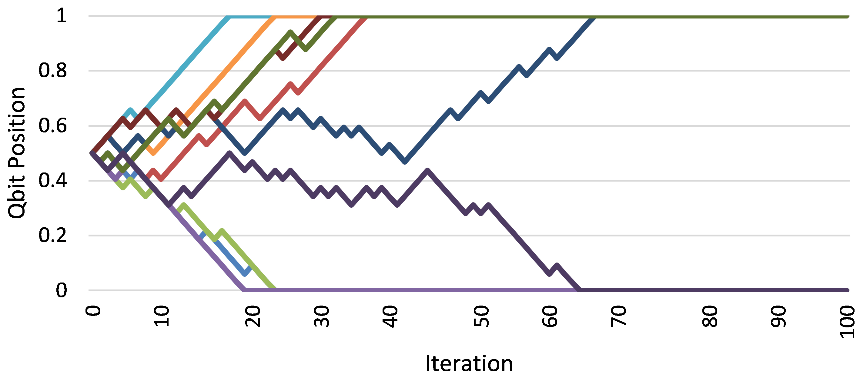

A simulation of 100 such random walks found saturation to either zero (53% of walks) or one (47% of walks) within a maximum of 99 simulations. Mean number of iterations until saturation was 36.82, with std. dev of 16.10. In practice the behaviour of the optimisation algorithm will only approximately follow this random walk model for the LSBs, but that could be enough to cause premature LSB convergence, especially when a large number of iterations are performed.

$\begin{array}[]{l}\begin{cases}{X_{t}<0}&{y_{t+1}=\max\left({0,y_{t}+X_{t}% \Delta\theta}\right)}\\ {X_{t}>0}&{y_{t+1}=\min\left({1,y_{t}+X_{t}\Delta\theta}\right)}\\ \end{cases},\\ X_{t}\sim\begin{cases}{-1,}&{p=1-y_{t}}\\ {\,1,}&{p=y_{t}}\\ \end{cases},\\ \end{array}$ (3)

where $X_{t}$ is a random variable with a Bernoulli distribution, with the probabilities for the two states being dependent on the random walk position $y_{t}$ at time $t$ . The step size for the rotation gate is $\Delta\theta$ .

In reality, the LSBs will exhibit some evolutionary pressure, varying according to the shape of the fitness landscape, but as illustrated in Fig. 1(a), the time line of the Qbit evolution shows that the LSBs can be observed to saturate early on in the process.

2.3 Improved bQIEA convergence performance for real value problems – HSB (Half Significant Bit)

One possible solution of these convergence problems is presented in [19], where the rotation gate operator has limits imposed that were slightly within the zero to one range. This means that, even late in the evolution, it is always possible to sample new bit values as the Qbits never completely saturate.

However, as we have analysed this premature convergence to be a problem of LSB evolution relative to MSB revolution, and inspired by early experimentation that failed to find much benefit from the constraint strategy, we present and test a method that explicitly constrains LSB Qbit rotation, relative to MSB Qbit rotation. When rotating a Qbit, we impose a limit upon the range that it can move to, based on the current value of a more significant bit, so that it cannot move to a more extreme value. This has the effect of delaying large movements in the LSBs until the MSBs have saturated.

Using the more significant immediate neighbour bit as a limiting condition made the convergence too slow, but picking a bit index that was half the position value of the Qbit being rotated (assuming bit index zero as the most significant one), gave acceptable results. This is a somewhat less aggressive limiting condition, which gives a compromise between premature convergence and overly slow convergence. Future work will be needed to identify the optimum index strategy. The adjusted formula for the rotation is given in Eq. 4, with the general algorithm code staying the same as for Classic. This modified algorithm is called HSB (Half Significant Bit) in this paper, and preliminary results of an evolution are shown in Fig. 1(b). The global and local migration rates $G=$ 20 and $L=$ 1, and the population subdivisions (5 subsets) are assumed the same as in the Classic method [18].

$\displaystyle Q_{i+1,j}=$ $\displaystyle\begin{cases}{\min\left({Q_{i,j}{+}\Delta\theta,\pi/4{+}\left|{Q_% {i,h}-\pi/4}\right|}\right),}&{\Delta\theta>0}\\ {\max\left({Q_{i,j}{+}\Delta\theta,\pi/4-\left|{Q_{i,h}-\pi/4}\right|}\right),% }&{\Delta\theta<0}\end{cases},$ $\displaystyle\mbox{where }j>0,h=\mbox{floor}\left({j/2}\right).$ (4)

Equation (4) applies the rotation but then compares the result to a more significant bit. This bit, $h$ , has a position index equal to one half of the index of the bit being modified, $j$ , rounded down to the nearest integer. The comparison is done to limit the range to be no more extreme than the more significant bit. The extremeness is determined by measuring the reference bit’s deviation for the central position $\pi$ /4. Bit index zero is modified according to the original Eq. 2 as there are no more significant bits relative to it.

3. Real QIEA (rQIEA)

In order to apply QIEA to real-value problems, numerous attempts have been made to develop real QIEA (rQIEA) [53], and we chose to include rQIEA in this investigation. A simple attempt at this is shown in [54] where the rotation angles from the Classic bQIEA are re-interpreted as actual solutions. This approach has the advantage of ease of implementation, and maintains the binary sampling metaphor while delivering real values. However, the sampling produces one of two options per dimension, rather than a range of values when a binary string is used. In our initial testing we did not produce satisfactory results using this algorithm on our test set. However, we found one algorithm called RCQIEA, presented in [55], to be well defined, to have good results on standard benchmarks, and to retain a meaningful proportion of the quantum metaphor. Therefore, we decided to include it in our study, along with a modification for improved performance.

3.1 The RCQIEA algorithm

Whereas Classic produces fresh solutions at each generation, RCQIEA stores and updates a candidate solution. Classic takes the inspiration of superposition and uses it to evolve a probability density function (pdf), as described by the probability angles for each bit. By not doing this directly, RCQIEA begins to move away from the original quantum metaphor. However, as we will describe shortly, the generation of new candidates through creep mutation, can be seen as using the candidate as a string of mean values for an evolving pdf.

At each iteration, a set of offspring $O_{j}$ is generated from each individual’s candidate $C_{i}$ using creep mutation with variances stored in a string $V_{i}$ . The values in $V_{i}$ are stored as angles and transformed into a pair $\alpha_{i}$ and $\beta_{i}$ in the same way as for the Classic. The offspring are generated in two subsets: one using $\alpha_{i}$ for the variances; and one using $\beta_{i}$ /5, to allow for both fine and coarse searching. The offspring are tested for fitness and if one is found to be better than the current candidate, it replaces that candidate. Otherwise, a rotation gate is applied to the variance angles in the same way as in Classic, but with a rotation step given in Eq. 5.

$\Delta\theta=\,{\rm sgn}\,\left({\alpha\beta}\right)\theta_{0}\exp\left({\frac% {\left|\beta\right|}{\left|\alpha\right|+\gamma}}\right),$ (5)

where $\alpha$ and $\beta$ are the angles as defined in Eq. 1, and $\theta_{0}$ and $\gamma$ are constants.

A cross-over operator is also applied during the evolution. For our investigation, we applied it four times during the course of each run ( $G=N$ /4), adopting the approach presented in [55]. The pseudo-code for the rQIEA presented here, is given in Algorithm 2.

3.2 Problems with rotation gate

In [55], the constants for Eq. 5 were specified as $\theta_{0}=0.4\pi$ and $\gamma=0.05$ . In the testing, the RCQIEA performed well for many functions. However, we detected values of large magnitudes for $\Delta\theta$ , which suggested a problem with the behaviour of the rotation gate. For example, if the angles are $\alpha=0.01$ and $\beta=0.99995$ (satisfying $\alpha^{2}+\beta^{2}=1$ ), then Eq. 5 produces a magnitude for $\Delta\theta$ in excess of 5.0e8. As a rotation angle in this context, such a magnitude for $\Delta\theta$ does not make sense, as it represents many complete rotations in one iteration. In effect this leads to somewhat random updates of the angle variables, and in turn, the variances for the creep mutation. A real example of these problematic delta values can be seen in Fig. 3.

Figure 3.

An example of the 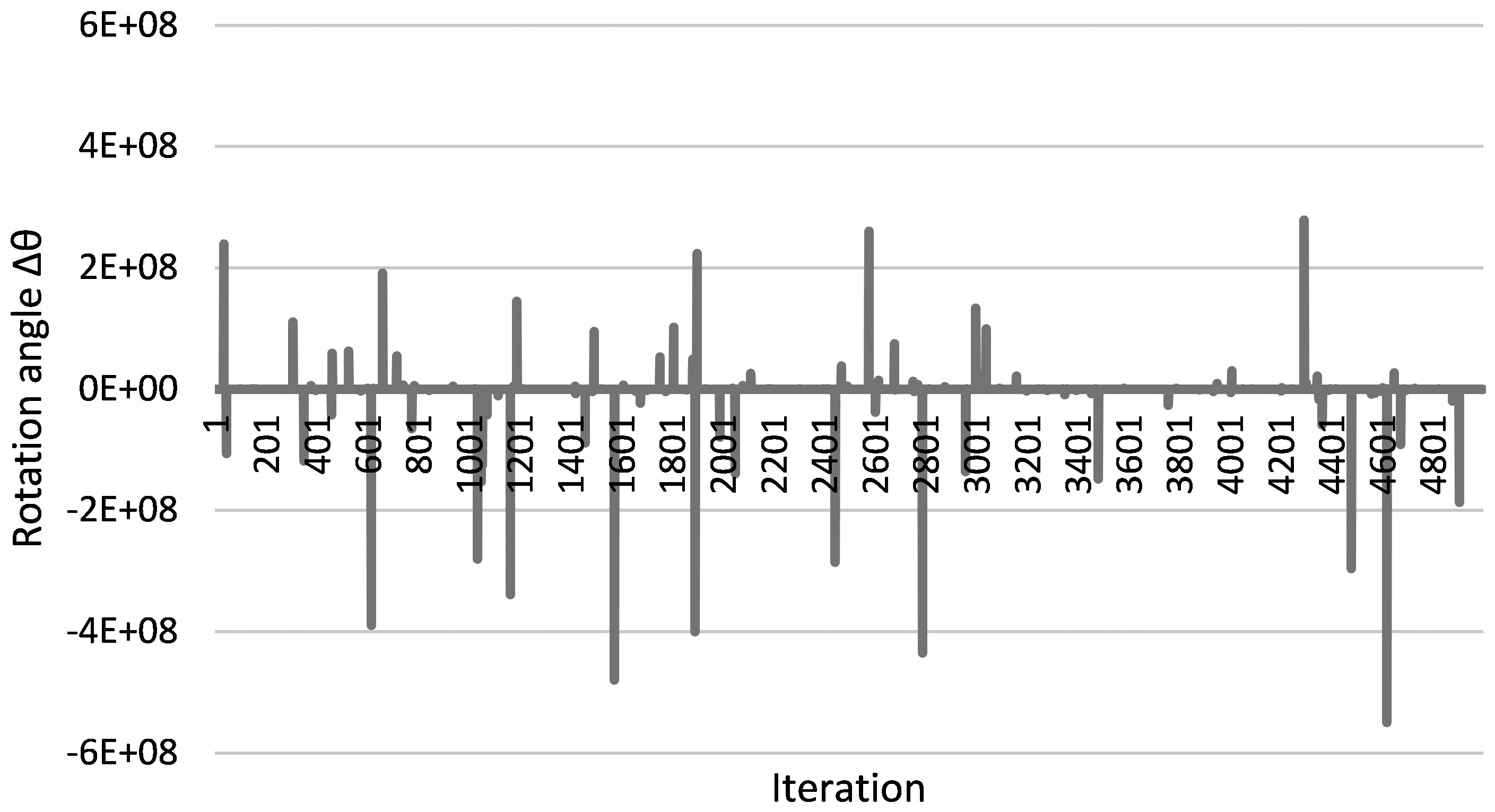$\Delta\theta$ values for the RCQIEA algorithm on the Griewank test function. The maximum magnitude should be $\pi$ /2, but very large values can be also observed.

3.3 Improving the rotation gate

To alleviate this problem, we developed a modified version of the rotation gate, keeping the rest of the RCQIEA algorithm (see Algorithm 2). We call this modified algorithm Stepwise Real QEA (SRQEA). The change rotates the angles by a constant magnitude in the rotation gate, as shown in Eq. 6.

$\Delta\theta=\,{\rm sgn}\,\left({\alpha\beta}\right)\pi/{250}.$ (6)

This change was motivated by making the update similar to the constant step size used in Classic, and in doing so, automatically avoiding problematic step sizes since they are now a fixed amount rather than a function of the state variables. Whereas Classic’s rotation gate affects the absolute probability of sampling a zero or one, the rotations in RCQIEA adjust the variance of repeated creep mutations. Since larger values are possible in this regime, we hypothesised that a smaller step size would be appropriate. Despite testing a range of alternative step sizes, we failed to identify a strong relationship between step size and algorithm performance, with $\pi$ /250 providing reasonable results. Future work is needed to quantify the step size/performance relationship, including testing a wider range of step sizes, more runs and more fitness functions. Also, we kept $G=N/4$ from [55], but other generation sizes could be investigated along with step size variants in the future.

4. Numerical simulation

Each algorithm was tested against several fitness functions. In accordance with the procedures outlined in [22], functions were tested with 10, 30 and 50 dimensions (except for the real-world problems which had specific dimension requirements), and each optimization run was performed 51 times, unless otherwise stated. The termination criterion was set to a number of function evaluations of 10000 $\times$ number of dimensions, unless otherwise stated. Given that more than one function evaluation per generation was performed for the rQIEA, their generations per run were adjusted accordingly.

The testing environment was a custom Windows MFC C $++$ programme running on Windows 7, with an Intel G2030 CPU, a Gigabyte Z68AP-D motherboard and 8 GB DDR3.

4.1 Test functions

Firstly, a set of traditional, basic functions, was taken from the first 13 functions presented in [50]. Additionally, a non-transformed basic version of Schwefel 7 [20] was used when comparing to data published for three recent QIEA [16, 20, 29], and a basic two dimensional problem from [46], when comparing another QIEA. A second set of more complicated functions was added from the first 20 functions defined in the CEC-2013 specification [22]. These are based on the traditional functions but are highly modified and transformed, including application of rotations. It should be noted that both sets share one function in common – the Sphere function. We duplicate the presentation of the results for this function in order to be consistent when comparing to other published results. Finally, real-world problems from CEC-2011 [11] were added: frequency modulated sound wave matching; atom configuration; and radar waveform parameter optimisation.

The frequency modulated sound wave matching problem optimises the constants of Eq. 7, so that the output of the wave, measured for integer $t=[0,100]$ , where $\theta=2\pi$ /100, matches the output of Eq. 8.

$\displaystyle y(t)=a_{1}\sin(\omega_{1}t\theta+a_{2}\sin(\omega_{2}t\theta$ $\displaystyle\quad+a_{3}\sin({\omega_{3}t\theta})))$ (7) $\displaystyle y(t)=1.0\sin(5.0t\theta-1.5\sin(4.8t\theta$ $\displaystyle\quad+2.0\sin({4.9t\theta}))),$ (8)

where $\alpha$ and $\omega$ are the constants to be optimised.

The Lennard-Jones atom potential configuration problem, aims to minimise the potential energy $V_{N}$ of a set of $N$ atoms with position $p_{i}=\left\{{x_{i},y_{i},z_{i}}\right\}$ according to Eq. 9.

$\begin{split}\displaystyle V_{N}\left(p\right)&\displaystyle=\sum_{i=1}^{N-1}{% \sum_{j=i+1}^{N}{\left({r_{ij}^{-12}-2r_{ij}^{-6}}\right)}},\\ \displaystyle r_{ij}&\displaystyle=\left\|{p_{j}-p_{i}}\right\|_{2}.\end{split}$ (9)

Finally, the radar polyphase pulse design problem seeks to minimise a function $f(x)$ based upon set of $n$ parameters $x=\{x_{1},\ldots,x_{n}\}$ according to Eq. 10.

$\hskip-19.916929pt\begin{split}\displaystyle f\left(x\right)&\displaystyle=% \max\left\{{\phi_{1}\left(x\right),\ldots,\phi_{2m}\left(x\right)}\right\},\\ \displaystyle\phi_{2i{-}1}\left(x\right)&\displaystyle=\sum_{j=i}^{n}\cos\left% (\sum_{k=\left|{2i{-}j{-}1}\right|{+}1}^{j}{x_{k}}\right),\\ &\displaystyle\qquad i=1,\ldots,n,\\ \displaystyle\phi_{2i}\left(x\right)&\displaystyle=0.5{+}\sum_{j=i{+}1}^{n}% \cos\left(\sum_{k=\left|{2i{-}j}\right|{+}1}^{j}x_{k}\right),\\ &\displaystyle\qquad i=1,\ldots,n{-}1,\\ \displaystyle m&\displaystyle=2n{-}1.\\ \end{split}$ (10)

4.2 Population size analysis

Before conducting an extensive evaluation of the proposed methods, an investigation into choosing a suitable population size was conducted. An initial run for 30 dimensions was performed for the optimisation algorithms on the non-real world functions, with a series of different population sizes being used. The number of individuals ranged from 5 to 50, in increments of five, but the total number of functions evaluations was kept to 300000. After running the simulations, the number of times an algorithm had a best performance (assessed just for that algorithm) was counted for each population size. A best performance occurred when it was the best, or equal best, minimum value or mean value for the fitness function of that optimisation algorithm.

Figure 4.

Population analysis for the QIEA: (a) Classic; (b) HSB; (c) RCQIEA; (d) SRQEA. For each algorithm, a simulation run was performed on the first 13 non-real world problems presented in [50] with 30 dimensions, with population sizes from 5 to 50. Then, for each algorithm in isolation, a count of best minimum and best mean values were produced for each population size (best as determined across all population sizes). The number of fitness evaluations was kept to 300000.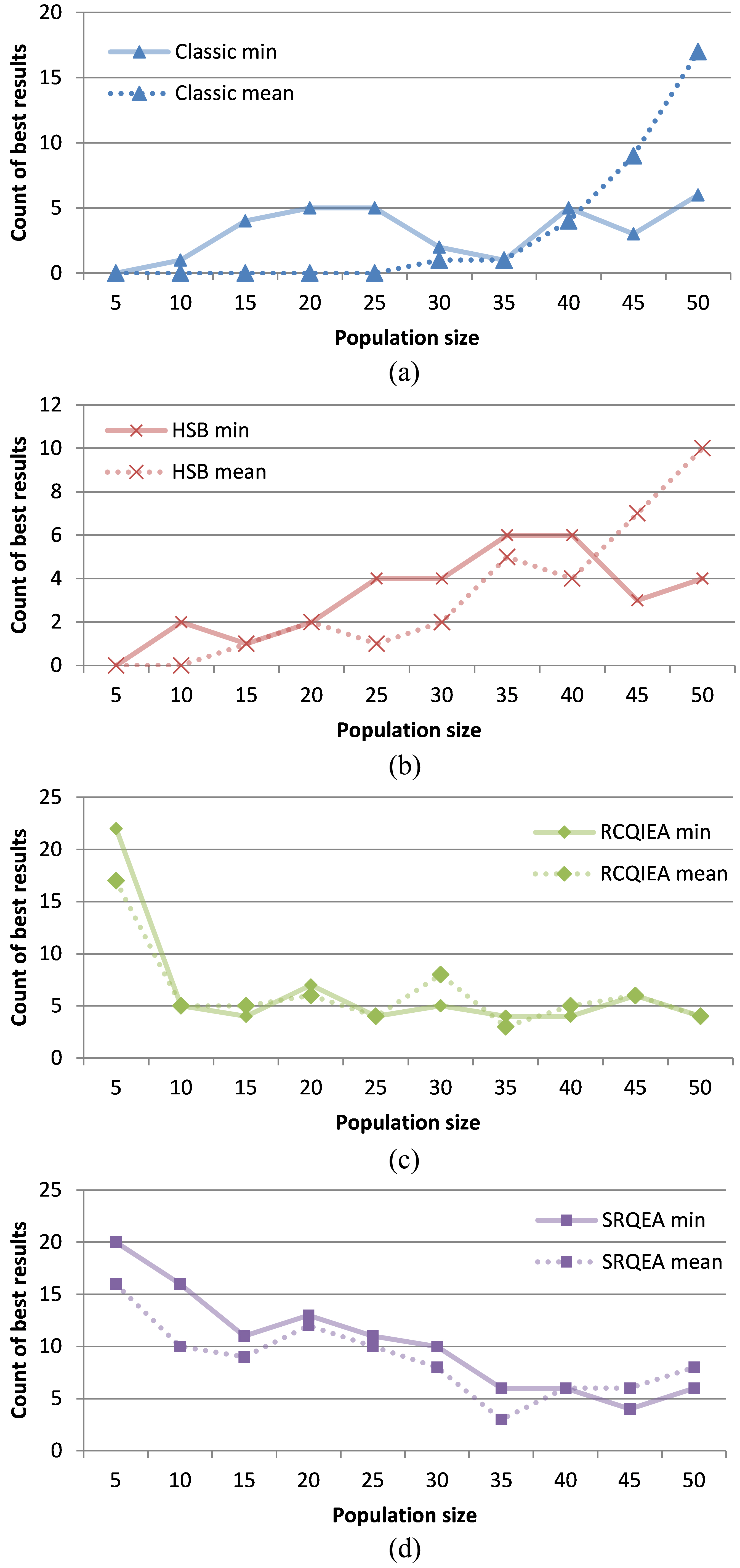

The results according to the best minimum and mean values found are shown in Fig. 4. Results for the bQIEA Classic and HSB are shown in Figs 4(a) and (b) respectively, and results for the rQIEA RCQIEA and SRQEA are shown in Figs 4(c) and (d) respectively.

Generally, the bQIEA performed better with higher population sizes, while the rQIEA were better with smaller population sizes. For Classic (Fig. 4(a)), the best minimum values were found more often with a population size of 50, with an additional peak at 20/25, while HSB (Fig. 4(b)) had a peak at 35/40 but reasonable performance from 25 to 50. When looking at the mean performance, both bQIEA improved with increasing population size, with the best being 50 for both. After combining these results, we chose to proceed with 50 individuals for both bQIEA algorithms in the later simulations and analysis. These results suggest bQIEA are biased towards exploitation and therefore require a larger population size to achieve good exploration.

For both rQIEA, the results (Figs 4(c) and (d)) were very clear – a population size of five performed the best for both minimum and mean values. RCQIEA had a sharp drop-off in performance above five, while SRQEA had a smoother decline with increasing population size. Based upon these results, a population size of five was chosen for both rQIEA. In contrast to the results for the bQIEA, these results suggest the rQIEA have relatively good exploration, so benefit from a small population in order to improve exploitation by increasing the number of function evaluations per individual.

4.3 Performance metrics

4.3.1 Summary statistics

To present a basic analysis and compare across publications, summary information is generated from error values (from the known minimum value) or absolute values if the global minimum is unknown. From the raw data, simple statistical measures such as minimum, mean and standard deviations are calculated and summarised, with lower values for each being preferred in the comparisons. Using the procedures outlined in [17], average mean performance was ranked and tested with a Friedman test, and pairwise significance tests were conducted with Shaffer’s static procedure. Additionally, for the majority of functions, pairwise comparisons between algorithms were performed on SPSS using the Mann-Whitney U test, with Bonferroni-Holm adjustment for multiple comparisons, to compare the distribution of error values found on each run when analysing one pair in isolation. However, this should be seen in the context of the pairwise tests as these single pairwise run comparisons do not take into account error propagation through multiple pairwise comparisons.

4.3.2 Success rates

Using metrics introduced in [10], a success rate and measure of time taken by the run to succeed (converging to a minimum) are calculated. Success Rate (SR) is calculated as the number of successful runs divided by the total number of runs. A run is regarded as successful if it finds an error below a predefined threshold.

4.3.3 Success performance

To measure the speed at which an algorithm obtains good results, a metric called Success Performance (SP) is calculated [10]. This is defined as SP $=$ (SNFEs) $*$ (number of total runs)/(number of successful runs), where SNFEs is the average number of function evaluations required by each successful run to reach the tolerance. A lower value of SP is preferred because it indicates a better combination of speed and consistency for the algorithm.

4.3.4 Timeline plots

In order to analyse the behaviour of the algorithms, graphical representations of their evolution are produced for every test function. Across all runs, for each iteration the mean error is calculated and plotted. So that the behaviour, with respect to the number of function evaluations, can be compared directly between the algorithms, and the time is normalised in the [0, 1] range.

4.3.5 Empirical cumulative probability distribution

Performance across all functions is summarised using the empirical cumulative probability distribution function (ECDF) method presented in [15]. An ECDF is constructed by firstly determining the performance of each algorithm on each test function, by comparing its mean error ME with the mean error achieved by the best algorithm, and formulating a normalized mean error NME (Eq. 11). Then, the distribution is formed by counting, for each value $x$ in the domain of the distribution, how many normalized means (across all test functions) were obtained below $x$ (Eq. 12). Normalizing and plotting these values produces a graph where superior algorithms reach the top of the chart faster than less well performing algorithms. In this analysis, all the test functions were included, as well as additional graphs for subsets (traditional, CEC-2013 and real-world).

$\displaystyle\textit{NME}_{A,f}=\frac{\textit{ME}_{A,f}}{\textit{ME}_{\textit{% best},f}+1},$ (11) $\displaystyle\textit{ECDF}(x)=\frac{1}{n_{A}\times n_{f}}\sum_{i=1}^{n_{A}}{% \sum_{j=1}^{n_{f}}{I({\textit{NME}_{i,j}\leqslant x})}}$ (12)

where $A$ and $f$ are the optimisation algorithm and the test function index respectively, $n_{A}$ and $n_{f}$ are the number of algorithms and test functions respectively.

5. Results and discussion

Examples of methods used to optimise CEC-2013 problems include Particle Swarm Optimization [51], Adaptive Differential Evolution [41, 44, 52], Mean Variance Mapping [37] and GA [14]. The methods for optimisation of the traditional test functions, covered in this work, include Evolutionary Programming [50], Particle Swarm Optimization [30], GA [26], and Hybrid Bee Colony/QEA [13]. This section presents the bQIEA and rQIEA results that we produced.

Table 1
Friedman test of average ranking of mean performance. Higher ranking is better

$p<$ 0.001
Algorithm	Ranking
Classic	1.50
HSB	2.25
RCQIEA	2.98
SRQEA	3.27

Table 2

Pairwise comparisons between Classic, HSB, RCQIEA and SRQEA, for average mean performance on 50 dimensions for functions 1 to 33. A Friedman test of average ranks gave $p<$ 0.001. Pairwise comparisons between the algorithms were then conducted using Shaffer’s static procedure and are listed below. All null hypotheses were rejected at the 10% level at least apart from RCQIEA vs SRQEA

Hypothesis			Unadjusted $p$	Shaffer’s $p$
Classic	vs	SRQEA	$<$ 0.001	$<$ 0.001
Classic	vs	RCQIEA	$<$ 0.001	$<$ 0.001
HSB	vs	SRQEA	0.002	0.005
Classic	vs	HSB	0.020	0.060
HSB	vs	RCQIEA	0.023	0.060
RCQIEA	vs	SRQEA	0.384	0.384

5.1 Pairwise statistical comparison of the QIEA

In Table 1 a Friedman test on average means for 50 dimensions rank Classic as the worst performer across the traditional and CEC-2013 functions, followed by HSB, RCQIEA, and lastly SRQEA as the best performer, with a statistical significant difference across the group ( $p<$ 0.001). A Shaffer’s pairwise test is presented in Table 2. All comparisons showed significantly differences apart from between RCQIEA and SRQEA (adjusted $p=$ 0.384). Furthermore the comparison between HSB and Classic, and HSB and RCQIEA were weakly significant (adjusted $p$ both 0.06). The other comparisons were highly significant (adjusted $p<$ 0.005). More work is needed to demonstrate a difference between SRQEA and RCQIEA by this measure, although other tests presented below are suggestive of better performance by SRQEA in addition to the better average mean ranking.

5.2 Statistical comparison of the QIEA on traditional test functions

In order to be useful optimization algorithms, the

Table 3
Summary statistics for the 13 traditional and 19 CEC-2013 test functions (duplicated 14 Sphere removed) with 50 dimensions and 500000 function evaluations. For each of the four optimization algorithms, the minimum, mean and standard deviation of the error values are presented after 51 runs. Best values are highlighted in bold type

Traditional and CEC-2013	bQIEA						rQIEA
functions 50 dimensions	Classic			HSB			RCQIEA			SRQEA
Function	Min	Mean	Std dev	Min	Mean	Std dev	Min	Mean	Std dev	Min	Mean	Std dev
01 Sphere	1.35E+03	3.35E+03	1.07E+03	1.81E+02	1.63E+03	7.16E+02	3.01E-04	5.81E-04	1.79E-04	0.00E+00	0.00E+00	0.00E+00
02 Schwefel-2.22	9.12E+01	1.67E+02	3.90E+01	4.92E+01	1.23E+02	3.17E+01	7.98E-02	1.08E-01	1.30E-02	0.00E+00	0.00E+00	0.00E+00
03 Schwefel-1.2	5.44E+05	2.20E+06	1.01E+06	1.48E+05	7.98E+05	4.56E+05	2.03E-01	4.26E-01	2.13E-01	0.00E+00	0.00E+00	0.00E+00
04 Schwefel-2.21	2.16E+01	3.63E+01	6.13E+00	1.83E+01	2.44E+01	4.01E+00	1.81E-01	3.05E-01	4.89E-02	2.00E-02	3.29E-02	7.54E-03
05 Rosenbrock	9.29E+06	2.81E+08	1.78E+08	7.79E+06	9.17E+07	7.77E+07	9.37E+00	1.27E+02	5.77E+01	4.49E-02	4.34E+01	3.09E+01
06 Step	1.22E+03	3.29E+03	1.41E+03	6.51E+02	1.72E+03	6.53E+02	0.00E+00	0.00E+00	0.00E+00	0.00E+00	0.00E+00	0.00E+00
07 Quartic	3.76E+06	6.42E+07	6.02E+07	6.57E+05	1.51E+07	1.33E+07	0.00E+00	0.00E+00	0.00E+00	0.00E+00	0.00E+00	0.00E+00
08 Schwefel-2.26	1.22E+02	3.21E+02	1.30E+02	4.15E+01	1.88E+02	8.73E+01	3.17E-05	6.60E-05	2.20E-05	0.00E+00	0.00E+00	0.00E+00
09 Basic Rastrigin	7.14E+01	1.04E+02	1.44E+01	3.06E+01	6.18E+01	1.06E+01	1.56E-04	2.89E-04	8.13E-05	0.00E+00	0.00E+00	0.00E+00
10 Basic Ackley	1.59E+01	1.93E+01	6.07E-01	1.42E+01	1.72E+01	1.12E+00	1.02E-02	1.66E-02	3.10E-03	0.00E+00	5.63E-07	3.26E-06
11 Basic Griewank	1.07E+01	2.92E+01	1.22E+01	3.64E+00	1.53E+01	5.86E+00	4.01E-04	8.45E-03	9.66E-03	0.00E+00	1.48E-02	2.59E-02
12 Penalised-1	1.04E+06	4.77E+07	3.66E+07	8.72E+01	1.09E+07	1.74E+07	0.00E+00	0.00E+00	0.00E+00	0.00E+00	0.00E+00	0.00E+00
13 Penalised-2	1.43E+07	1.38E+08	9.05E+07	5.21E+05	2.95E+07	3.73E+07	0.00E+00	0.00E+00	0.00E+00	0.00E+00	0.00E+00	0.00E+00
15 R HC elliptic	5.30E+07	1.17E+08	4.11E+07	4.55E+07	1.02E+08	3.28E+07	5.84E+06	1.15E+07	3.01E+06	1.55E+06	2.96E+06	6.43E+05
16 Rotated bent cigar	1.38E+10	3.21E+10	8.83E+09	4.85E+09	1.90E+10	1.04E+10	1.18E+03	6.45E+06	2.26E+07	4.98E-02	1.58E+05	1.08E+06
17 Rotated discus	5.44E+04	8.77E+04	1.68E+04	1.02E+04	2.40E+04	7.45E+03	1.38E+05	1.92E+05	2.88E+04	1.14E+05	1.75E+05	2.47E+04
18 Different powers	5.98E+02	4.90E+03	3.35E+03	9.52E+01	1.14E+03	1.46E+03	1.57E-03	4.14E-03	1.94E-03	0.00E+00	0.00E+00	0.00E+00
19 Rotated Rosenbrock	1.12E+02	3.10E+02	1.01E+02	1.04E+02	2.72E+02	9.86E+01	2.98E+01	4.51E+01	3.43E+00	2.38E+01	4.19E+01	7.54E+00
20 Rotated Schaffers-F7	1.44E+02	1.83E+02	2.18E+01	1.21E+02	1.78E+02	2.47E+01	1.79E+02	2.54E+02	1.22E+02	1.47E+02	2.46E+02	9.28E+01
21 Rotated Ackley	2.11E+01	2.12E+01	4.08E-02	2.10E+01	2.12E+01	3.58E-02	2.10E+01	2.11E+01	3.74E-02	2.10E+01	2.11E+01	4.68E-02
22 Rotated Weierstrass	4.46E+01	5.27E+01	4.77E+00	4.07E+01	5.27E+01	4.47E+00	5.71E+01	6.34E+01	3.36E+00	6.16E+01	6.74E+01	3.76E+00
23 Rotated Griewank	5.36E+02	1.05E+03	2.68E+02	4.03E+02	8.27E+02	2.22E+02	1.54E+00	2.25E+00	3.02E-01	2.71E-02	1.31E-01	4.96E-02
24 Rastrigin	7.36E+01	1.33E+02	2.56E+01	5.48E+01	7.99E+01	1.82E+01	5.83E-04	1.10E-03	3.38E-04	0.00E+00	0.00E+00	0.00E+00
25 Rotated Rastrigin	2.41E+02	3.69E+02	7.14E+01	2.33E+02	3.86E+02	8.38E+01	3.58E+02	6.08E+02	1.25E+02	4.60E+02	6.85E+02	1.38E+02
26 NC rotated Rastrigin	3.95E+02	5.23E+02	7.68E+01	3.51E+02	5.60E+02	1.15E+02	4.71E+02	6.30E+02	9.74E+01	5.01E+02	6.89E+02	1.01E+02
27 Schwefel-7	3.85E+02	1.17E+03	3.62E+02	1.43E+02	5.36E+02	2.46E+02	2.96E-02	8.57E-02	2.41E-02	9.99E-02	6.71E-01	2.94E-01
28 Rotated Schwefel-7	5.68E+03	7.73E+03	9.96E+02	5.12E+03	7.33E+03	9.92E+02	4.37E+03	6.25E+03	7.15E+02	4.69E+03	6.22E+03	6.23E+02
29 Rotated Katsuura	8.49E-01	2.02E+00	5.86E-01	1.26E+00	1.91E+00	4.11E-01	8.74E-01	1.64E+00	3.49E-01	8.93E-01	1.83E+00	4.41E-01
30 Lunacek bi-Rastrigin	1.31E+02	2.68E+02	6.63E+01	9.44E+01	1.65E+02	4.14E+01	3.82E-02	9.98E-02	3.51E-02	0.00E+00	1.96E-04	1.40E-03
31 R Lunacek bi-Rastrigin	3.41E+02	6.49E+02	1.27E+02	4.52E+02	6.51E+02	1.08E+02	3.05E+02	4.80E+02	7.87E+01	4.53E+02	6.12E+02	9.30E+01
32 RE Griewank Rosen.	9.91E+01	5.90E+02	7.94E+02	7.21E+01	4.55E+02	5.85E+02	5.73E+01	1.45E+02	4.66E+01	1.46E+02	2.91E+02	6.26E+01
33 RE Schaffers-F6	1.51E+01	1.93E+01	2.47E+00	1.51E+01	1.84E+01	1.95E+00	2.05E+01	2.43E+01	5.97E-01	1.90E+01	2.44E+01	7.68E-01

Table 4

Summary statistics for CEC-2011 real world problems. For each of the four optimization algorithms, the minimum, mean and standard deviation of the error values are presented after 51 runs. Best values are highlighted in bold type. Function evaluations were limited to 150000

Func	bQIEA						rQIEA
tion	Classic			HSB			RCQIEA			SRQEA
	Min	Mean	Std dev	Min	Mean	Std dev	Min	Mean	Std dev	Min	Mean	Std dev
FM	4.42E-02	1.34E+01	6.11E+00	3.01E-03	1.07E+01	6.99E+00	2.71E-04	1.57E+01	5.78E+00	0.00E+00	1.70E+01	4.68E+00
L-J5	$-$ 1.21E+01	$-$ 9.62E+00	1.49E+00	$-$ 1.22E+01	$-$ 1.03E+01	1.55E+00	$-$ 1.27E+01	$-$ 1.18E+01	1.03E+00	$-$ 1.27E+01	$-$ 1.21E+01	1.02E+00
L-J10	$-$ 2.72E+01	$-$ 1.80E+01	4.03E+00	$-$ 2.67E+01	$-$ 1.95E+01	3.79E+00	$-$ 3.08E+01	$-$ 2.26E+01	3.87E+00	$-$ 3.18E+01	$-$ 2.41E+01	4.23E+00
Radar	1.58E+00	2.00E+00	1.97E-01	1.40E+00	1.91E+00	2.02E-01	1.50E+00	2.00E+00	2.31E-01	1.59E+00	2.11E+00	2.10E-01

QIEA must find solutions close to the optimum, as represented by small error values. We start by looking at the performance on the traditional test functions, with minimum, mean and standard deviation data presented in Table 3 (functions 1–13) for 50 dimensions.

These functions are reasonably smooth, at least locally, and therefore obtaining a good error score will require good exploitation abilities of the algorithm. In Section 2 we highlighted the difficulties for Classic in optimising the LSBs, and we would expect this to be reflected in poor minimum values as the exploitation would be hampered. For both bQIEA, most solutions had errors of magnitude above 1e-01, although some of the fitness functions had large constant factors (e.g., Rosenbrock has a constant factor of 100) so absolute values require a degree of interpretation. Even so, with four minima of magnitude over 1e06 at 50 dimensions for Classic and four above 1e05 for HSB, and similar means performance, the bQIEA do not have particularly impressive results for the traditional batch.

For the traditional test functions, HSB had equal or better minimum values than Classic at 50 dimensions, although the magnitudes were generally similar, except for 50 dimension Penalised-1 where HSB had a much better value than Classic. HSB With a statistically significant, although weak (adjusted $p=$ 0.06) difference in average mean performance (Table 2) this completes a picture of consistently better performance for HSB versus Classic, suggesting both that the LSB problems of Classic hampered its performance, and that our tested solution of limiting the LSB probability saturation was successful. Testing the bQIEA at 10 and 30 dimensions produced very similar results.

Despite apparent functional performance by the bQIEA, the two rQIEA were substantially better - most minima had magnitudes of less than 1e-01. In the Shaffer pairwise comparison of average mean performance (Tables 1 and 2), Classic was outperformed significantly by both rQIEA (adjusted $p<$ 0.001), and HSB was outperformed strongly by SRQEA (adjusted $p=$ 0.005) and weakly by rQIEA (adjusted $p=$ 0.06). RCQIEA found smaller than 1e-08 solutions (clamped to 0.00 in the results) for Step, Quartic, Penalised-1 and Penalised-2 in all tested dimensions. Despite RCQIEA performing well on these test functions, it was eclipsed by SRQEA. With the exception of Schwefel-2.21 and Rosenbrock, SRQEA obtained clamped 0.00 minima results for all of the functions, in all dimensions. Furthermore, in a statistical test of run distributions (Mann-Whitney U with Bonferroni-Holm adjusted), SRQEA was better than RCQIEA for 8 of the traditional functions, with no significant results the other way round. The superior performance of the real algorithms over their binary counterparts is unsurprising, given the application to real-value problems, but the superior performance of SRQEA justifies our modification of the rotation gate for these functions.

5.3 Statistical comparison of the QIEA on CEC-2013 test functions

As CEC-2013 is a set of real-value problems, some being modified versions of the functions from the traditional set tested here, we predicted that a similar pattern of results would be generated, with the rQIEA dominating the bQIEA. Although HSB outperformed Classic, and SRQEA outperformed RCQIEA, the performance of the bQIEA compared to the rQIEA was very different from its previous performance (see Table 3 functions 15–33).

For several of the test functions – Rotated Discus, Rotated Schaffers-F7, Rotated Weierstrass, Rotated Rastrigin, Non-continuous Rotated Rastrigin, Rotated Schwefel 7, Rotated Katsuura, Rotated Expanded Grienwank-Rosenbrock and Rotated Expanded Schaffers-F6, one of the bQIEA had the best performance for one or more dimensions tested. Although the relative difference between minima was lower when the bQIEA performed best, compared to when the rQIEA were best, there were 6 functions at 50 dimensions for which HSB had significantly better run result distributions than SRQEA (by Mann-Whitney U/Bonferroni-Holm). The positive results of the bQIEA are significant and surprising, given that they can outperform the rQIEA on some real-value benchmark functions.

The CEC-2013 functions are highly manipulated versions of traditional basic functions (many based on the traditional test functions used in this paper). The manipulations include rotations, scalings and non-linear transforms. We hypothesise that it is these transformations that allow the bQIEA to perform well and suggest that this could happen in one of two possible ways. Firstly, the transformations may increase the nonlinear interactions between dimensions, producing a fitness landscape that is very rough, and therefore more resembling a discrete space at scales above the very small. These search spaces may be suited to the binary methods presented here, possibly possessing similarities to the combinatorial problems that bQIEA have been successful with (e.g., Knapsack [18]). Alternatively, the search pattern may be the key. In the rQIEA, the search space is traversed using creep mutations with distances drawn from a normal distribution, while the movement in the bQIEA is performed using multi-scaled jumps as the bits flip between zero and one and move the search to an adjacent binary partition at the scale of the significance of the bit. This binary space partitioning could reflect, to some degree, the underlying structure of the search spaces.

For the CEC-2013 set of test functions, the bQIEA achieved several minimum scores with a magnitude of 1e02 or less and, given that the test functions often contain large constants (1e06), it could be argued that they performed better on the more difficult test functions than on the traditional set of functions. It would be interesting to see if this scales, so that the bQIEA have increasingly better relative performance as the fitness landscape becomes more complex. HSB appears to scale better than Classic, achieving 6 best minima performances across all four QIEA for 50 dimensions, compared to one for Classic. Furthermore, when comparing HSB to SRQEA for run distributions (by Mann-Whitney U/Bonferroni-Holm), SRQEA had more statistically significant advantages, but HSB achieved superior results for six test functions at 50 dimensions.

Although SRQEA performed the greatest, in terms of number of best minimum values found and the ability to find threshold zero error values for some CEC-2013 functions (which none of the other algorithms managed to do), when looking at the general performance across all of the functions and algorithms, the picture was somewhat more mixed. A heat map of best minimum values, scaled relatively from the best performing algorithm to the worst on each test function, is presented in Fig. 5. In this plot, judging by the number of darker rectangles, RCQIEA performs well, arguably outperforming SRQEA. From the raw data in Table 3, it can be seen that when the performances of the rQIEA are close, SRQEA produces better results than RCQIEA, but this is not generally noticeable in the heat map, where the larger degrees of magnitude produced by the bQIEA obscure the rQIEA differences. Summarising the raw data and the heat map, it can be said that RCQIEA had a slightly better minima performance across the test functions, on average, but SRQEA was able to produce much better individual scores for some functions. Furthermore, SRQEA had superior run distributions than RCQIEA (by Mann-Whitney U/Bonferroni-Holm), giving better average performance from run to run, although caution should be noted as in the group test of pairwise comparisons, the results between the two rQIEA was not significant (Table 2). The more random nature of the rotation gate of RCQIEA may produce desirable search characteristics for the CEC-2013 test functions, at the expense of more exploitation.

Figure 5.

Heat map of best values found, normalised for each function, by the QIEA on the CEC-2013 test functions. For each test function, the relative performance for each algorithm is plotted, with a green (zero) rectangle indicating best performance, and a light-green (one) rectangle indicating worst performance.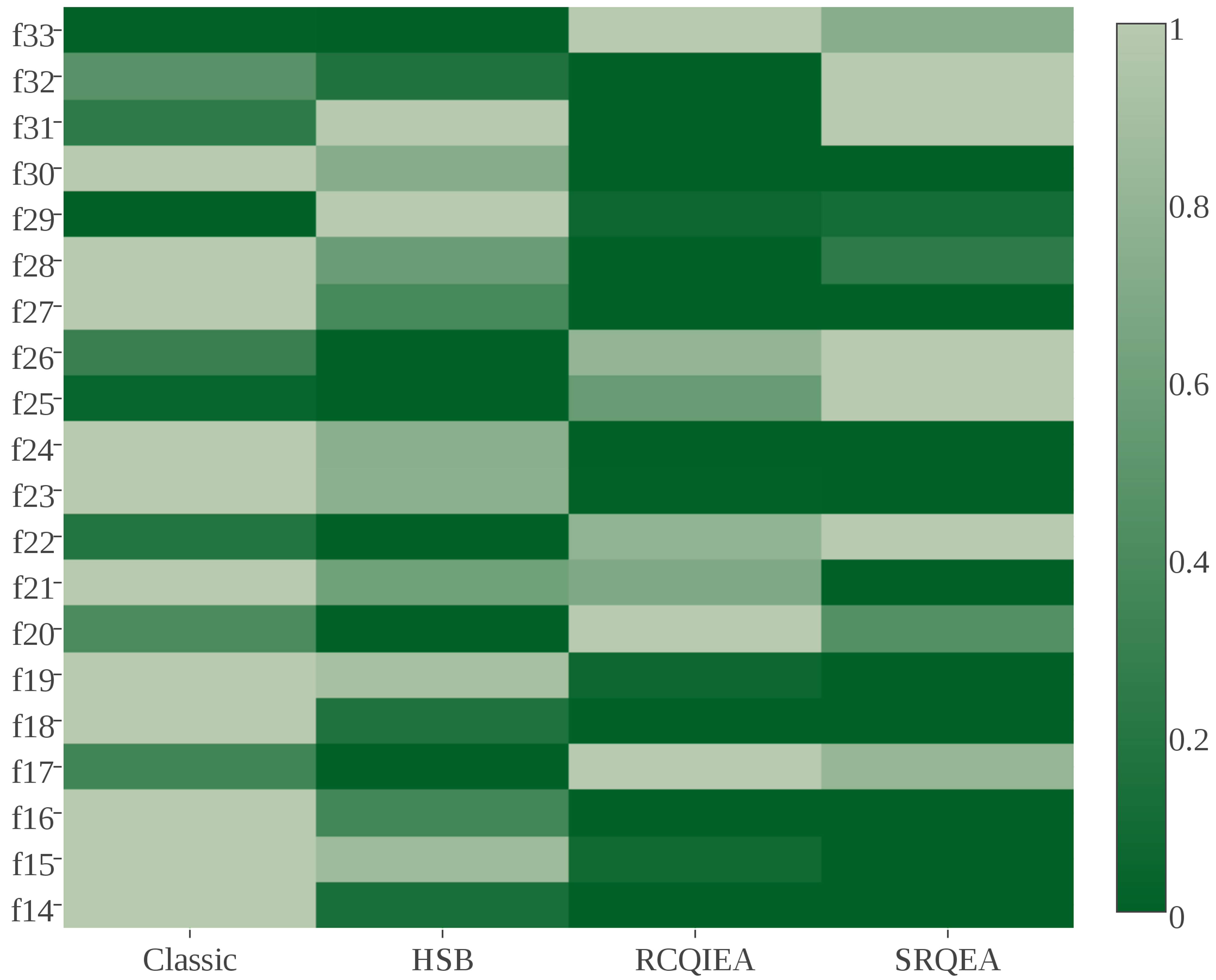

Figure 6.

Empirical cumulative probability distribution function of mean errors across (a) CEC-2013, and (b) real-world all test functions, comparing the four QIEA. The horizontal axis shows normalised mean score, and the vertical axis shows cumulative probability. The faster the approach to 1 in the vertical direction, the better the performance.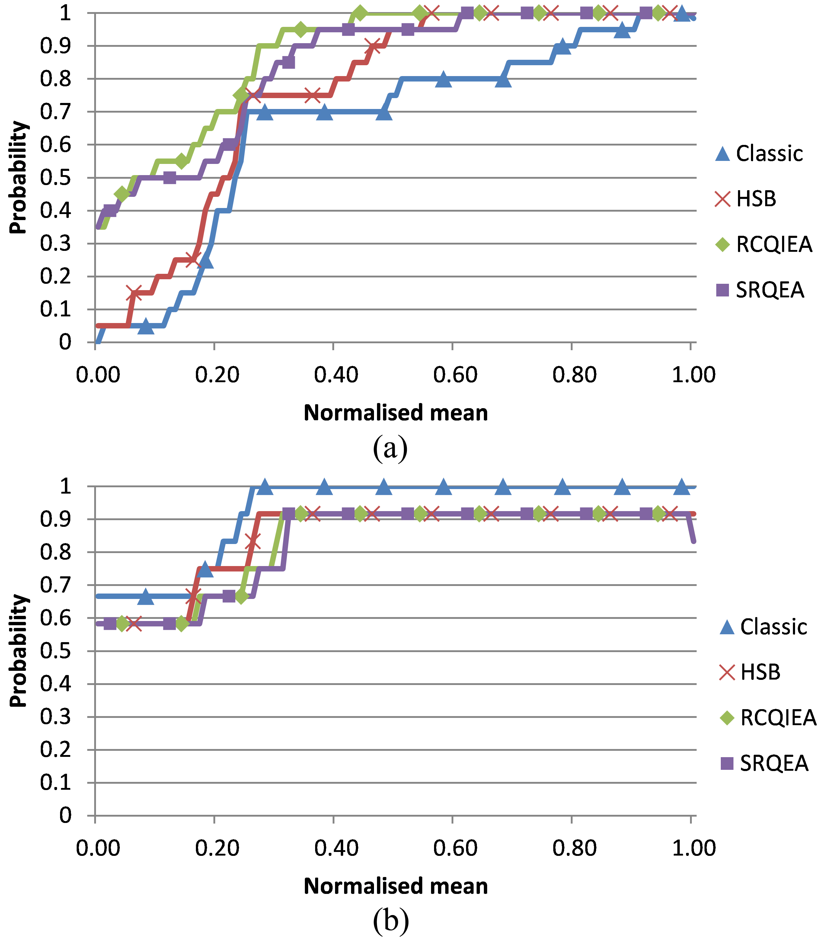

5.4 Statistical comparison of the QIEA on real world test functions

For the CEC-2011 real-world problems, converging to the minima was best for the rQIEA (Table 4), with SRQEA having the best scores for three of the functions. However, for the Radar Polly Phase problem HSB had the best result, and shared the number of best means equally with SRQEA. The nested functions of the Frequency Modulation and Radar Polly Phase problems suggest a highly nonlinear search space, so these results are consistent with our findings and interpretations of the performance of the bQIEA on the CEC-2013 functions.

Finally, we present a summary of algorithms’ mean performance across multiple test functions in Fig. 6. The plots show a cumulative normalised count of how many functions possess a normalised mean performance for that algorithm, below a given value. The sooner the plot reaches 1.0 in the vertical axis, the better the algorithm performs (as this indicates a high probability of achieving low mean error values).

The best performance on the traditional test functions (not shown) is dominated by the two rQIEA methods, which can also be seen for all of the test functions taken together (not shown), with Classic performing poorly for both of those cases. However, for the CEC-2013 functions HSB is much closer (Fig. 6(a)), catching up sooner with the rQIEA in the plot, although it starts with poorer results, indicating a low probability of producing very low mean scores across the function set. The performance of RCQIEA compared to SRQEA for CEC-2013 is in line with the results presented in the heat map (Fig. 5). SRQEA outperforms RCQIEA for low mean values, but takes a slight lead for normalised means between 0.2 and 0.4. For the real-world test functions (Fig. 6(b)), the situation is completely reversed, with Classic performing the best, followed by HSB.

Summarising the ECDF and the results given in Tables 1–4, we can conclude that, although the rQIEA have superior best performance (minimum values found),the bQIEA algorithms do have good mean performance, often superior to their real-value counterparts. Again, it is with the more complicated CEC-2013 and real-world CEC-2011 functions that the bQIEA perform at their best, often outperforming the rQIEA.

Figure 7.

Timeline evolution of mean error values. The mean error for each generation was calculated across each of the 51 runs, for every test function, and plotted for 51 dimensions on (a) Rotated Griewank, and (b) Schwefel-2.21. Each graph plots time normalized evolutions, comparing the relative performance of the optimization algorithms.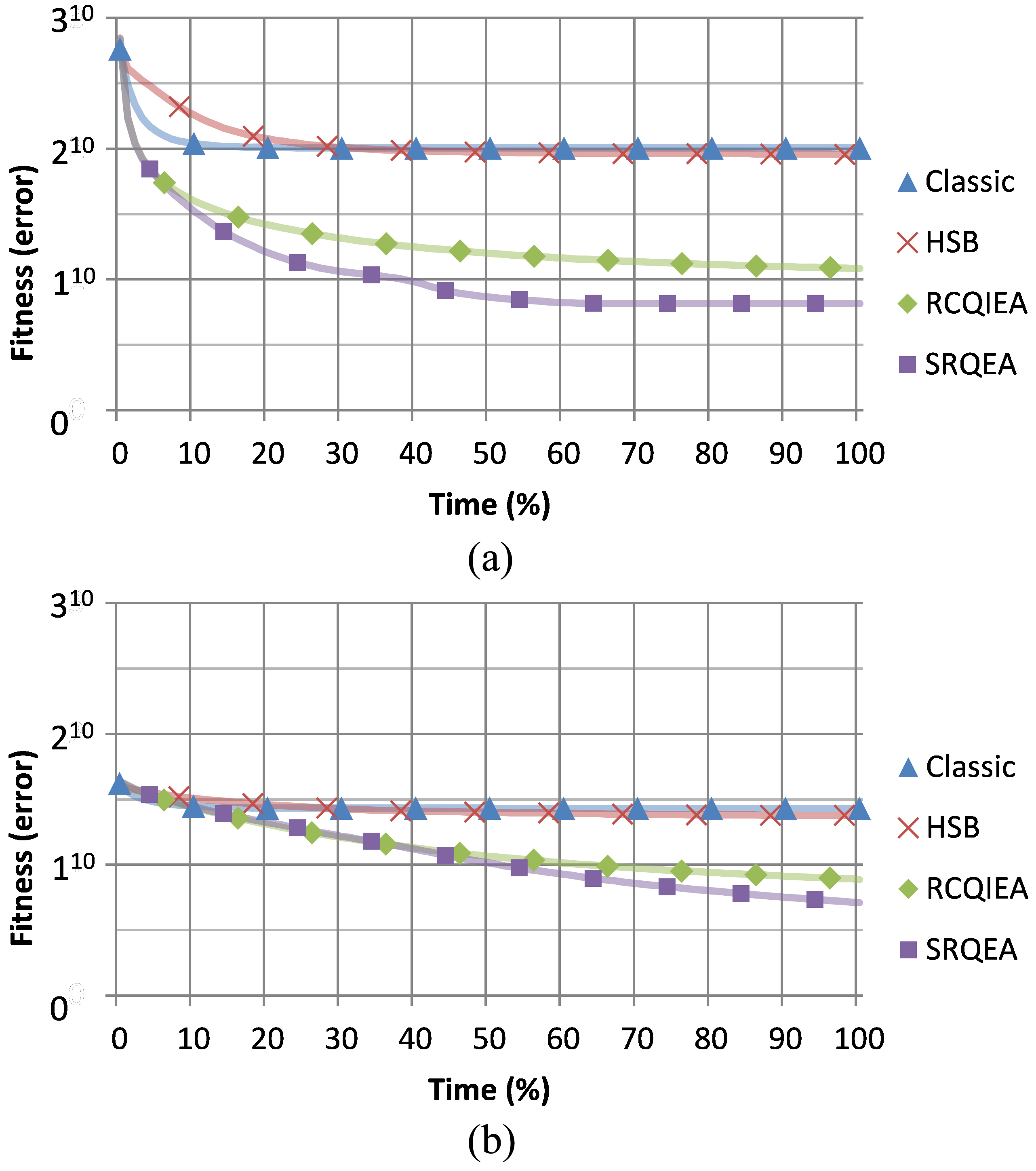

Table 5

Comparison between SRQEA, Fast Evolutionary Programming (FEP) [50], and MADE [33] on the traditional test functions. The SRQEA performed better than FEP, but was inferior to MADE for four of the functions. Best values are highlighted in bold type

30 dimensions	SRQEA				FEP			MADE
Function	Evals	Min	Mean	Std dev	Evals	Mean	Std dev	Evals	Mean	Std dev
1 Sphere	300000	0.00E+00	0.00E+00	0.00E+00	150000	8.10E-03	7.70E-04	150000	0.00E+00	0.00E+00
2 Schwefel-2.22	300000	0.00E+00	0.00E+00	0.00E+00	200000	8.10E-03	7.70E-04	150000	0.00E+00	0.00E+00
3 Schwefel-1.2	300000	0.00E+00	0.00E+00	0.00E+00	500000	1.60E-02	1.40E-02	200000	0.00E+00	0.00E+00
4 Schwefel-2.21	300000	3.51E-03	6.16E-03	1.56E-03	500000	3.00E-01	5.00E-01	500000	0.00E+00	0.00E+00
5 Rosenbrock	300000	1.04E-02	8.86E+01	1.80E+02	2000000	5.06E+00	5.87E+00	500000	3.97E-01	1.63E+00
6 Step	300000	0.00E+00	0.00E+00	0.00E+00	150000	0.00E+00	0.00E+00	500000	0.00E+00	0.00E+00
7 Quartic	300000	0.00E+00	0.00E+00	0.00E+00	300000	7.60E-03	2.60E-03	300000	1.24E-03	3.78E-04
8 Schwefel-2.26	300000	0.00E+00	0.00E+00	0.00E+00	900000	1.50E+01	5.26E+01	200000	0.00E+00	0.00E+00
9 Basic Rastrigin	300000	0.00E+00	0.00E+00	0.00E+00	500000	4.60E-02	1.20E-02	300000	0.00E+00	0.00E+00
10 Basic Ackley	300000	0.00E+00	9.20E-01	4.01E+00	150000	1.80E-02	2.10E-03	150000	0.00E+00	0.00E+00
11 Basic Griewank	300000	0.00E+00	2.06E-02	2.25E-02	200000	1.60E-02	2.20E-02	200000	0.00E+00	0.00E+00
12 Penalised-1	300000	0.00E+00	0.00E+00	0.00E+00	150000	9.20E-06	3.60E-06	300000	0.00E+00	0.00E+00
13 Penalised-2	300000	0.00E+00	0.00E+00	0.00E+00	150000	1.60E-04	7.30E-05	300000	0.00E+00	0.00E+00

Table 6

Comparison of success rates (SR) and speed of convergence (SP), between RCQIEA, SRQEA and 4 differential evolution algorithms, for the 13 traditional test functions with 30 dimensions. The threshold (1E-08, except of 1E-02 for Quartic) determines the point at which a run is a success. Best values are highlighted in bold type. Function evaluations are kept to 300000

Function	RCQIEA		SRQEA		jDE		SDE		JADE		MADE
	SP	SR	SP	SR	SP	SR	SP	SR	SP	SR	SP	SR
1 Sphere	–	0	2.48E+05	1	5.93E+04	1	3.91E+04	1	3.04E+04	1	2.29E+04	1
2 Schwefel-2.22	–	0	7.19E+05	1	8.16E+04	1	5.31E+04	1	5.61E+04	1	3.64E+04	1
3 Schwefel-1.2	–	0	3.56E+05	1	3.37E+05	1	–	0	7.17E+04	1	1.34E+05	1
4 Schwefel-2.21	–	0	–	0	2.99E+05	1	4.72E+05	0.44	–	0	1.27E+05	1
5 Rosenbrock	–	0	–	0	5.89E+06	0.08	–	0	1.22E+05	0.92	1.97E+05	0.92
6 Step	7.77E+04	1	4.27E+04	1	2.27E+04	1	1.44E+04	1	1.16E+04	1	7.89E+03	1
7 Quartic	1.37E+05	1	4.35E+04	1	1.12E+05	1	8.34E+04	1	2.97E+04	1	2.83E+04	1
8 Schwefel-2.26	–	0	2.12E+05	1	7.85E+04	1	5.50E+04	1	1.00E+05	1	6.00E+04	1
9 Basic Rastrigin	–	0	2.53E+05	1	1.17E+05	1	6.14E+05	0.36	1.31E+05	1	1.14E+05	1
10 Basic Ackley	–	0	1.54E+06	0.63	9.02E+04	1	5.95E+04	1	4.75E+04	1	3.55E+04	1
11 Basic Griewank	–	0	8.50E+05	0.31	6.21E+04	1	4.07E+04	1	3.30E+04	1	2.41E+04	1
12 Penalised-1	5.61E+04	1	3.85E+04	1	5.40E+04	1	3.66E+04	1	2.95E+04	1	2.03E+04	1
13 Penalised-2	3.85E+04	1	3.30E+04	1	5.76E+04	1	3.77E+04	1	2.95E+04	1	2.19E+04	1

5.5 Evolution properties of the QIEA

Mean error values per generation (averaged across the 51 runs) are shown for two functions in Fig. 7. For most functions, Classic outperformed HSB early on the evolution, but tends to stall earlier and is generally overtaken by HSB at around the 30% (of the total number of generations) time point (for example, see the Rotated Griewank function timeline in Fig. 7(a)). This gives additional support to our argument that Classic was prematurely converging when applied to real-value problems, and justifies our approach when formulating the HSB adaptation. However, it should also be noted that HSB also usually approaches an approximately zero gradient relatively early on (50% of time or less), implying there is further need to improve premature convergence.

For the majority of cases where SRQEA outperformed RCQIEA, their early performances were very similar, but SRQEA would establish a lead from typically the 10–30% time mark (see Rotated Griewank in Fig. 7(a)). We interpret this as indicating that our corrected rotation formula allowed a more refined search in later stages. Both rQIEA demonstrated a clear non-zero gradient at the end of the timeline in several of the plots (such as Fig. 7(b)). This suggests they are capable of finding significantly better results if the algorithm is run for longer. As the plots display the fitness to the 10 ${}^{\rm th}$ root, this is relevant for fine convergence to the optimal value, indicating room for improvement of precision.

In order to compare the speed of evolution for the QIEA on functions for which zero minima were obtained, success rates (SR) and success performances (SP) were calculated for RCQIEA and SRQEA for those test functions, using four threshold values: 1e-02, 1e-04, 1e-06 and 1e-08. The data are presented in Table 7. In almost all cases, SRQEA outperformed RCQIEA, with the only exception being the success rate for the basic Griewank function at the 1e-02 threshold. The SP metric gives the mean number of function evaluations per success, adjusted in order to penalise low success rates. In conclusion, the data show that SRQEA provides superior success rates, and quicker convergence than RCQIEA.

5.6 Comparison of QIEA with published results

As the best performing QIEA on the traditional test functions, we compare SRQEA to two other algorithms – FEP [50] and MADE [10] (Table 5). Comparison is made difficult by varying numbers of function evaluations across the published methods, but in general, SRQEA outperformed FEP except for the Rosenbrock, Ackley and Griewank functions where FEP had a superior mean and standard deviation. MADE was better than SRQEA for Schwefel-2.21, Rosenbrock, Ackley and Griewank, but SRQEA beat MADE for Quartic and matched it for all of the other functions. Unfortunately, best minimum values found were not published for either algorithm, but since MADE produced several zero means, it is clear those results would have been good as well.

The exploitation abilities of RCQIEA and SRQEA were compared to data published on a set of differen-

Table 7
Success rates (SR) and success performance (SP) for the test functions at 30 dimensions, which reached a threshold of 1e-8 by one of the quantum algorithms, for different success thresholds: 1e-2; 1e-4; 1e-6; and 1e-8. SR ranges from 0 (no successes) to 1 (all runs where successful) and SP gives a measure of average number of iterations needed to achieve the threshold, adjusted in order to penalise algorithms with low success rates. SRQEAoutperformed RCQIEA for all functions and for all thresholds. Function evaluations were kept to 300000

30 dimensions	RCQIEA								SRQEA
	1.00E-02		1.00E-04		1.00E-06		1.00E-08		1.00E-02		1.00E-04		1.00E-06		1.00E-08
Function name	SR	SP	SR	SP	SR	SP	SR	SP	SR	SP	SR	SP	SR	SP	SR	SP
Sphere	1.00	3.52E+05	0.02	5.91E+07	0.00	–	0.00	–	1.00	5.65E+04	1.00	1.04E+05	1.00	1.65E+05	1.00	2.48E+05
Schwefel 222	0.00	–	0.00	–	0.00	–	0.00	–	1.00	1.27E+05	1.00	2.82E+05	1.00	4.79E+05	1.00	7.19E+05
Schwefel 12	0.00	–	0.00	–	0.00	–	0.00	–	1.00	1.12E+05	1.00	1.75E+05	1.00	2.60E+05	1.00	3.56E+05
Step	1.00	7.77E+04	1.00	7.77E+04	1.00	7.77E+04	1.00	7.77E+04	1.00	4.27E+04	1.00	4.27E+04	1.00	4.27E+04	1.00	4.27E+04
Quartic	1.00	1.37E+05	1.00	1.37E+05	1.00	1.37E+05	1.00	1.37E+05	1.00	4.34E+04	1.00	4.35E+04	1.00	4.35E+04	1.00	4.35E+04
Schwefel 226	1.00	1.78E+05	1.00	8.54E+05	0.00	–	0.00	–	1.00	4.28E+04	1.00	7.94E+04	1.00	1.36E+05	1.00	2.12E+05
Basic rastrigin	1.00	2.83E+05	0.18	6.57E+06	0.00	–	0.00	–	1.00	1.05E+05	1.00	1.28E+05	1.00	1.78E+05	1.00	2.53E+05
Basic ackley	0.06	1.95E+07	0.00	–	0.00	–	0.00	–	0.94	5.66E+05	0.92	7.12E+05	0.88	9.39E+05	0.63	1.54E+06
Basic griewank	0.53	1.07E+06	0.00	–	0.00	–	0.00	–	0.43	1.83E+05	0.31	3.83E+05	0.31	5.82E+05	0.31	8.50E+05
Penalised 1	1.00	5.61E+04	1.00	5.61E+04	1.00	5.61E+04	1.00	5.61E+04	1.00	3.85E+04	1.00	3.85E+04	1.00	3.85E+04	1.00	3.85E+04
Penalised 2	1.00	3.85E+04	1.00	3.85E+04	1.00	3.85E+04	1.00	3.85E+04	1.00	3.30E+04	1.00	3.30E+04	1.00	3.30E+04	1.00	3.30E+04
Diff. powers	0.98	5.25E+05	0.00	–	0.00	–	0.00	–	1.00	6.47E+04	1.00	1.37E+05	1.00	2.52E+05	1.00	3.80E+05
Rastrigin	1.00	4.41E+05	0.00	–	0.00	–	0.00	–	1.00	1.66E+05	1.00	1.87E+05	1.00	2.33E+05	1.00	3.01E+05
Lun. bi-rastrigin	0.00	–	0.00	–	0.00	–	0.00	–	0.96	4.48E+05	0.94	5.17E+05	0.94	5.54E+05	0.94	6.09E+05

Table 8

Comparison of HSB and SRQEA with five QIEA: HRCQEA; RQEA; NQPSO; QGAXM; and CQGA. Comparisons to HRCQEA, RQEA and NQPSO were standardised to the five functions used for HRCQEA [25], whereas for QGAXM and CQGA comparisons were made for all fitness functions presented. Values less than 1e-08 have been clamped to zero. Minimum scores for the compared algorithms are listed where available or where they can be deduced from zero means. Number of runs and function evaluations (FE) have been matched, except for HRCQEA (*) where only 300000 evaluations were performed per run. Best minimums are highlighted in bold except for the CQGA comparison which was a maximisation problem

Method	Compared algorithm				HSB		SRQEA
	Func	Dim	Min	Mean	Min	Mean	Min	Mean
HRCQEA 50 runs $*$ 2400000 FE	Sphere	30	0.00E+00	0.00E+00	1.40E+01	6.37E+02	0.00E+00	0.00E+00
	Rastrigin	30	0.00E+00	0.00E+00	1.62E+01	4.15E+01	0.00E+00	0.00E+00
	Ackley	30	1.70E-07	1.70E-07	1.02E+01	1.66E+01	0.00E+00	9.20E-01
	Schwefel 7	30	3.90E-04	3.90E-04	2.91E+02	7.10E+02	0.00E+00	2.60E+02
	Griewank	30	0.00E+00	0.00E+00	1.83E+00	7.69E+00	0.00E+00	2.06E-02
RQEA 25 runs 500000 FE	Sphere	50	0.00E+00	0.00E+00	3.80E+02	1.65E+03	0.00E+00	0.00E+00
	Rastrigin	50	–	5.32E-07	4.61E+01	6.36E+01	0.00E+00	0.00E+00
	Ackley	50	0.00E+00	0.00E+00	1.09E+01	1.72E+01	0.00E+00	8.36E-08
	Schwefel 7	50	–	5.80E-03	5.84E+02	1.64E+03	0.00E+00	6.40E+02
	Griewank	50	0.00E+00	0.00E+00	4.78E+00	1.77E+01	0.00E+00	2.36E-02
NQPSO 30 runs 200000 FE	Sphere	30	0.00E+00	0.00E+00	9.37E+01	5.79E+02	0.00E+00	0.00E+00
	Rastrigin	30	0.00E+00	0.00E+00	2.07E+01	3.54E+01	0.00E+00	0.00E+00
	Ackley	30	0.00E+00	0.00E+00	1.57E+01	1.94E+01	1.64E-08	1.49E+00
	Schwefel 7	30	–	3.80E+03	4.46E+02	8.17E+02	0.00E+00	2.89E+02
	Griewank	30	0.00E+00	0.00E+00	2.13E+00	6.90E+00	0.00E+00	2.54E-02
QGAXM 30 runs 10000 FE	Sphere	50	1.90E-01	4.20E-01	7.80E+04	9.43E+04	1.40E+01	8.43E+01
	Rastrigin	50	1.67E+04	1.35E+05	6.41E+02	6.92E+02	1.67E+05	2.09E+06
	Rosenbrock	50	3.20E+02	4.61E+02	2.19E+10	4.50E+10	1.87E+01	2.86E+01
	Griewank	50	1.44E+00	2.22E+00	6.66E+02	8.56E+02	1.12E+00	1.58E+00
CQGA, 10 runs, 8000 FE	Complex binary	2	$-$ 17.3503	–	$-$ 17.4503	$-$ 17.4486	$-$ 17.4503	$-$ 17.4503

tial algorithms (DE) [10]. The results are presented in Table 6, using the success rate (SR) and success performance (SP) metrics. In general, the DE algorithms achieved success more often, and quicker than the rQIEA. The SRQEA is superior to RCQIEA for these metrics, achieving better success rates, and reaching the threshold more quickly (better SP). These results (Table 6) represent the weakest performance for the QIEA in this paper, and indicate room for improvement in their search and exploitation abilities for the traditional test functions. However, it should be noted that success rates were based on very low thresholds (usually 1e-08) and therefore may not be important in practical cases. Unfortunately, when comparing to MADE we did not have data on its application to the CEC-2013 functions, so we cannot argue if these conclusions hold for the more complicated test functions. However, the reader should note that a modified version of MADE – Super-fit MADE (SMADE) has now been produced and applied to the CEC-2013 benchmarks [5].

A comparison of SRQEA with five different QIEAs is given in Table 8: a hybrid quantum PSO algorithm HRCQEA [20], a region based QIEA RQEA [29], a hybrid quantum PSO with neighbourhood search NQPSO [16], and two hybrid quantum GAsQGAXM [33] and CQGA [46]. The five fitness functions used in [20] where available in [29, 16], so were chosen for comparison. When comparing to QGAXM and CQGA, the evaluated fitness functions were matched in their entirety, including a two-dimensional problem from [46].

The number of runs and the maximum function evaluations were matched, except for HRCQEA, where our algorithms performed only 300000 evaluations. It can be concluded that SRQEA is as good as, or better than these algorithms for finding the functions’ minimum values, with the exception when against QGAXM, where SRQEA was better for the multi-modal problems, but worse for Sphere and Rosenbrock. Mean performance was less impressive, and suggests a weakness in exploitation capabilities of SRQEA for the basic functions, especially when using the low number of function evaluations when compared to QGAXM. In the next section though, evidence of a very good exploration for the more complicated CEC-2013 functions will be presented. The CQGA algorithm used binary encoding, but with only 20 bits, and was beaten not just by SRQEA, but by HSB as well. Otherwise, HSB only achieved superior performance for Rastrigin against QGAXM and SRQEA.

Table 9

SRQEA compared to SPSO-2011 and a GA algorithm for the CEC-2013 functions with 50 dimensions and 500000 FEs. The SRQEA matched or outperformed the other two algorithms on best value found (Min) for 11 test functions. Best values are highlighted in bold type

50 dimensions	SRQEA			SPSO-2011 [11]			GA [13]
Function	Min	Mean	Std dev	Min	Median	Std dev	Min	Median	Mean	Std dev
14 Sphere [duplicated]	0.00E+00	0.00E+00	0.00E+00	0.00E+00	0.00E+00	3.18E-13	0.00E+00	0.00E+00	0.00E+00	0.00E+00
15 R HC elliptic	1.55E+06	2.96E+06	6.43E+05	3.79E+05	6.80E+05	1.87E+05	1.74E+05	4.28E+05	4.76E+05	2.14E+05
16 Rotated bent cigar	4.98E-02	1.58E+05	1.08E+06	2.00E+07	4.37E+08	9.47E+08	2.55E+06	3.44E+07	1.06E+08	1.49E+08
17 Rotated discus	1.14E+05	1.75E+05	2.47E+04	3.22E+04	5.10E+04	8.72E+03	4.90E-01	2.25E+00	3.33E+00	4.88E+00
18 Different powers	0.00E+00	0.00E+00	0.00E+00	0.00E+00	0.00E+00	5.41E-05	0.00E+00	0.00E+00	4.77E+04	1.70E+05
19 Rotated rosenbrock	2.38E+01	4.19E+01	7.54E+00	1.84E+01	4.35E+01	2.41E+01	3.66E+01	4.36E+01	4.72E+01	1.40E+01
20 Rotated schaffers-F7	1.47E+02	2.46E+02	9.28E+01	5.61E+01	8.64E+01	1.53E+01	1.51E+01	3.97E+01	4.17E+01	1.83E+01
21 Rotated ackley	2.10E+01	2.11E+01	4.68E-02	2.10E+01	2.11E+01	4.25E-02	2.11E+01	2.12E+01	2.12E+01	3.98E-02
22 Rotated weierstrass	6.16E+01	6.74E+01	3.76E+00	4.52E+01	5.40E+01	6.74E+00	5.21E+01	7.53E+01	7.43E+01	3.97E+00
23 Rotated griewank	2.71E-02	1.31E-01	4.96E-02	1.00E-01	4.00E-01	2.38E-01	2.71E-02	9.36E-02	1.05E-01	7.09E-02
24 Rastrigin	0.00E+00	0.00E+00	0.00E+00	1.50E+02	2.30E+02	4.18E+01	1.49E+01	5.37E+01	5.57E+01	2.23E+01
25 Rotated rastrigin	4.60E+02	6.85E+02	1.38E+02	1.62E+02	2.35E+02	4.87E+01	5.07E+01	9.75E+01	9.83E+01	2.45E+01
26 NC rotated rastrigin	5.01E+02	6.89E+02	1.01E+02	3.20E+02	4.28E+02	6.22E+01	1.04E+02	1.86E+02	1.93E+02	5.30E+01
27 Schwefel-7	9.99E-02	6.71E-01	2.94E-01	5.51E+03	7.26E+03	8.53E+02	1.06E+03	2.30E+03	2.55E+03	1.14E+03
28 Rotated schwefel-7	4.69E+03	6.22E+03	6.23E+02	5.68E+03	7.92E+03	1.14E+03	6.20E+03	8.24E+03	9.84E+03	3.19E+03
29 Rotated katsuura	8.93E-01	1.83E+00	4.41E-01	1.40E+00	2.00E+00	3.87E-01	2.23E+00	3.76E+00	3.68E+00	3.88E-01
30 Lunacek bi-rastrigin	0.00E+00	1.96E-04	1.40E-03	2.08E+02	3.11E+02	6.62E+01	8.25E+01	1.13E+02	1.15E+02	2.00E+01
31 R Lunacek bi-rastrigin	4.53E+02	6.12E+02	9.30E+01	1.70E+02	2.91E+02	6.24E+01	8.83E+01	1.32E+02	1.68E+02	1.02E+02
32 RE griewank rosenb.	1.46E+02	2.91E+02	6.26E+01	1.70E+01	3.72E+01	1.20E+01	3.60E+00	9.02E+00	8.92E+00	3.17E+00
33 RE schaffers-F6	1.90E+01	2.44E+01	7.68E-01	1.99E+01	2.27E+01	1.19E+00	1.99E+01	2.36E+01	2.35E+01	8.02E-01

Table 10

Comparison of performance on real-world problems between SRQEA and three alternative algorithms – MADE-WS [33], EA-DE-Memetic [37] and an adaptive differential evolutionary algorithm [38]. The starred value has been clamped to zero as it was below the threshold of 1E-08 (used in our simulations). Best values are highlighted in bold type. Function evaluations are kept to 150000

Function	SRQEA			MADE-WS			EA-DE-Memetic			Adaptive DE
	Min	Mean	Std dev	Min	Mean	Std dev	Min	Mean	Std dev	Min	Mean	Std dev
FM	0.00E+00	1.70E+01	4.68E+00	–	8.81E-01	2.47E+00	0.00E+00*	3.81E+00	5.21E+00	0.00E+00	4.85E+00	6.69E+00
L-J 5	$-$ 1.27E+01	$-$ 1.21E+01	1.02E+00	–	$-$ 9.09E+00	8.83E-02	–	–	–	–	–	–
L-J 10	$-$ 3.18E+01	$-$ 2.41E+01	4.23E+00	–	$-$ 2.66E+01	8.64E-01	$-$ 2.84E+01	$-$ 2.59E+01	2.24E+00	$-$ 2.80E+01	$-$ 2.68E+01	2.11E+00
Radar	1.59E+00	2.10E+00	2.09E-01	–	–	–	2.20E+02	2.20E+02	0.00E+00	2.20E+02	2.20E+02	0.00E+00

Table 9 shows the performance of SRQEA against two algorithms that were applied to the CEC-2013 fitness functions [22]. The two algorithms compared are a particle swarm optimization algorithm SPSO-2011 [51] and a genetic algorithm GA [14]. SRQEA was chosen for comparison as, overall, it was the best performing QIEA tested here, in terms of minimum values found.

Looking at all dimensions, all three algorithms achieved some best performances. However, SPSO-2011 performed least well, having fewer best minimum results, and most of those being joint equal with one or both of the other algorithms. The main competition for SRQEA came from the GA. For 10 dimensions it achieved 16 best performances, with SRQEA only achieving seven. For 30 dimensions GA scored 12 best performances, while the SRQEA reached 8, but for 50 dimensions, SRQEA took the lead with 11 compared to 9 best results for the GA. This demonstrates better scaling with increased number of dimensions for SRQEA than for the GA. Mean performance was similarly distributed across all dimensions but SRQEA showed improved standard deviation performance again for 50 dimensions, outperforming the other algorithms substantially. This shows a more consistent relative performance at higher dimensions for SRQEA as well as better minima and means.

The poorer performance of SPSO-2011 (Table 9) and the better performance of the GA may suggest that the recombinatorial properties of the cross-over operator may aid the search pattern for the CEC-2013 functions. This may be consistent with either of our hypotheses for why the bQIEA performed relatively well against the rQIEA – either treating the rougher space as more discrete and looking for recombination, or navigating through hops (swapping genes in the case of GA, and flipping bits in the case of the bQIEA). Although overall SRQEA was better, it would be interesting to see how bQIEA perform against rQIEA and other algorithms on even more complex search spaces.

A comparison between SRQEA and two alternative algorithms, when applied to the real-world problems is shown in Table 10. For the frequency modulation wave matching problem, MADE-WS [10] had the best mean and standard deviation. Unfortunately, the authors did not report a minimum value. SRQEA outperformed the hybrid algorithm [38] and the DE algorithm [2], in terms of mean and standard deviation, while equalling the best minimum performance. The mean and standard deviation were worse but comparable with the MADE-WS results.

For the Lennard-Jones problems, SRQEA again established the best minimum values, but MADE-WS did not have a comparable values published. SRQEA did have the best mean value for Lennard-Jones5 but only outperformed the hybrid algorithm for Lennard-Jones10.

For the radar waveform parameter specification problem, SRQEA was the clear winner. The published results [38, 2] both gave a suspiciously poor value though, and it may be worth considering whether there were issues in using shared code for the function evaluations. The problem was directly tackled in [32] where a variable neighbourhood search algorithm gave a minimum value of 8.58e-01 which was better than that achieved by the SRQEA.

6. Conclusion

When applied to real-value optimization tasks, all of the QIEA tested and validated in this investigation were successful, in that they were able to produce acceptable to excellent error values (with respect to the complexity of the test functions). Binary QIEA are a direct implementation of the quantum computing metaphor, which is built around repeated sampling of binary strings, analogous to superposition of states on a set of quantum bits. The Qbit probabilities define a probability distribution that elegantly specifies both the region of the best solution found so far, and the variance of the search radius. As the probabilities saturate, the mean position of the search becomes clearly defined, and the variance of the search narrows.

Although the original Classic algorithm performed relatively poorly on the optimization tasks examined here, our modification (HSB) did substantially improve the results. In many instances it outperformed RCQIEA, especially for the more difficult CEC-2013 test functions. The timeline plots highlighted the premature convergence of Classic (a), giving further justification for our choice of modification, which was developed in response to our analysis of individual bit evolution. By explicitly limiting the saturation of less significant bits to the magnitude of saturation of more significant bits, HSB avoids the problems that Classic encountered for real-value problems, although zero gradients in the latter half of some timeline plots suggest there is still room for improvement. The population size results (Figs 4(a) and (b)) also suggest exploration issues, as the bQIEA benefit from a larger population size for a fixed number of function evaluations.

Our modification to the rotation gate produced superior results, particularly with regards to the final ability to exploit the search space (Tables 1–4) and the speed of exploitation (Table 7), although from the heatmap of Fig. 5 it would appear the average performance across the functions is slightly compromised. This suggests the superior exploitation may come at the expense of some exploration capability. As well as being beneficial in this specific implementation, it would be interesting for future work to explore the possibility of using the modified rotation in other algorithms, as a way of adjusting search variance.

When compared to other published results, our modified algorithms were predominantly competitive for the more complex CEC-2013 functions (Table 9). For the traditional test functions, SRQEA was superior than recently published QIEA in terms of best minimum reached (Table 8), although mean performance was mixed, and our algorithms were generally outperformed by other published results (in particular, the DE algorithms [10], Tables 5 and 6). However, timeline plots (Fig. 7) suggest the rQIEA may continue to improve if left for longer. It would therefore be interesting to see if these algorithms are suitable for increasingly complicated test functions, where longer processing times are to be expected. Both HSB and SRQEA outperformed a bQIEA applied to a real value problem (Table 8).

Surprisingly, the bQIEA appeared to perform better for the more complex CEC-2013 and the real-world test functions (Tables 1–4). We have speculated that this may be because either the transferred search space begins to resemble the binary space portioning that the bQIEA generate, or that the search hops at different scales (depending on bit significance) may result in more suitable search patterns when compared to rQIEA or other algorithms. The ability of bQIEA to combine different scales, through bit manipulation, may explain their improved performance on these more sophisticated tasks. As more complex fitness functions are published in the future, it would be worth including bQIEA (and perhaps other binary optimisation algorithms) in attempting to optimise them. It should be noted however, that the bQIEA require more computation per iteration due to longer strings being processed. The importance of this will depend on the demands of the fitness evaluation, with fast fitness functions being more negatively affected by the bQIEA overhead.

QIEA, and rQIEA in particular, provide a good starting point for optimization. Deficiencies, when compared to competing algorithms, were largely down to fine exploitation, with results being of a similar degree of magnitude in error (Table 5). Future work would be beneficial on improving exploration for SRQEA, or further reducing the premature convergence for HSB. This may be achieved through an analysis of the effect of changing algorithm parameters (as discussed below), or by including the QIEA in hybrid algorithms with a two-stage exploration and exploitation process. Using the configuration of step size and other parameters presented here, the two rQIEA are more orientated towards exploration than exploitation. This is demonstrated by the populations analysis (Fig. 4), which showed they both benefitted from a small population size for a given number of function evaluations (thereby increasing the number of iterations per individual). The bQIEA in contrast performed best with a larger population size and so appear to be balanced more towards exploitation than exploration.

One final advantage of QIEA is the low number of parameters they require for the main part of their implementation. Generally, only the number of individuals and step size for the rotation gate are needed. The rQIEA presented here also include a parameter for the number of children produced in each generation. For all of the investigated algorithms, the number of individuals and rotation gate step magnitude need specifying. The bQIEA also have parameters for local and global update rates, while rQIEA have crossover rates. How these affect the overall performance was not evaluated. The rQIEA also add a parameter for the number of offspring spawned at each iteration. Again, changing this was not analysed and further investigation into the optimisation of these parameters would be worth conducting.

References

AlRashidi

El-Hawary

. A survey of particle swarm optimization applications in electric power systems. IEEE Trans Evol Comput. 2009 Aug; 13(4): 913-918.

Asafuddoula

Ray

Sarker

. An adaptive differential evolution algorithm and its performance on real world optimization problems. In: IEEE Congress on Evolutionary Computation (CEC). 2011; 1057-1062.

Babu

Das

Patvardhan

. Real-parameter quantum evolutionary algorithm for economic load dispatch. Gener Transm Distrib IET. 2008; 2: 22-31.

Campomanes-Ávarez

Cordón

Damas

. Evolutionary multi-objective optimization for mesh simplification of 3D open models. Integrated Computer-Aided Engineering. 2013 Oct; 20(4): 375-390.

Caraffini

Neri

Cheng

Zhang

Picinali

Iacca

, et al. Super-fit multicriteria adaptive differential evolution. In: 2013 IEEE Congress on Evolutionary Computation. 2013; 1678-1685.

Caraffini

Neri

Picinali

. An analysis on separability for Memetic Computing automatic design. Inf Sci. 2014 May 1; 265: 1-22.

Chabuk

Reggia

Lohn

Linden

. Causally-guided evolutionary optimization and its application to antenna array design. Integrated Computer – Aided Engineering. 2012 Jan 1; 19(2): 111-124.

Chaoyong

Yongjuan

Jianguo

. A real-coded quantum-inspired evolutionary algorithm for global numerical optimization. 2008; 1160-1164.

Chen

J-F

T-J

. A computational intelligence optimization algorithm: Cloud drops algorithm. Integrated Computer-Aided Engineering. 2014 Apr; 21(2): 177-188.

10.

Cheng

Zhang

Caraffini

Neri

. Multicriteria adaptive differential evolution for global numerical optimization. Integrated Computer-Aided Engineering. 2015 Apr; 22(2): 103-107.

11.

Das

Suganthan

. Problem definitions and evaluation criteria for CEC 2011 competition on testing evolutionary algorithms on real world optimization problems. Jadavpur Univ Nanyang Technol Univ Kolkata. 2010.

12.

Das

Suganthan

. Differential Evolution: A Survey of the State-of-the-Art. IEEE Trans Evol Comput. 2011 Feb; 15(1): 4-31.

13.

Duan

H-B

C-F

Xing

Z-H

. A hybrid artificial bee colony optimization and quantum evolutionary algorithm for continuous optimization problems. Int J Neural Syst. 2010 Feb 1; 20(01): 39-50.

14.

Elsayed

Sarker

Essam

. A genetic algorithm for solving the CEC’2013 competition problems on real-parameter optimization. In: IEEE Congress on Evolutionary Computation (CEC). 2013; 356-360.

15.

Epitropakis

Tasoulis

Pavlidis

Plagianakos

Vrahatis

. Enhancing differential evolution utilizing proximity-based mutation operators. IEEE Trans Evol Comput. 2011 Feb; 15(1): 99-119.

16.

Liu

Zhang

Deng

. Quantum behaved particle swarm optimization with neighborhood search for numerical optimization. Math Probl Eng. 2013 Oct 24; e469723.

17.

García

Herrera

. An extension on “statistical comparisons of classifiers over multiple data sets” for all pairwise comparisons. J Mach Learn Res. 2008 Dec 9; 2677-2694.

18.

Han

K-H

Kim

J-H

. Quantum-inspired evolutionary algorithm for a class of combinatorial optimization. Evol Comput IEEE Trans On. 2002; 6: 580-593.

19.

Han

K-H.

, Kim

J-H.

,Quantum-inspired evolutionary algorithms with a new termination criterion, H ε gate, and two-phase scheme. IEEE Trans Evol Comput. 2004 Apr; 8(2): 156-169.

20.

Hossain

Hashem

MMA

. A generalized hybrid real-coded quantum evolutionary algorithm based on particle swarm theory with arithmetic crossover. Int J Comput Sci Inf Technol. 2010 Aug 20; 2(4): 172-187.

21.

Hsu

W-Y

. Application of quantum-behaved particle swarm optimization to motor imagery EEG classification. Int J Neural Syst. 2013 Jul 3; 23(06): 1350026.

22.

Liang

. Problem definitions and evaluation criteria for the cec 2013 special session on real-parameter optimization. Tech Re 201212 Comput Intell Lab. Zhengzhou Univ. Zhengzhou China. 2013.

23.

Joly

Verstraete

Paniagua

. Integrated multifidelity, multidisciplinary evolutionary design optimization of counterrotating compressors. Integrated Computer-Aided Engineering. 2014 Jul; 21(3): 249-261.

24.

Kociecki

Adeli

. Two-phase genetic algorithm for size optimization of free-form steel space-frame roof structures. J Constr Steel Res. 2013 Nov; 90: 283-296.

25.

Kociecki

Adeli

. Two-phase genetic algorithm for topology optimization of free-form steel space-frame roof structures with complex curvatures. Eng Appl Artif Intell. 2014 Jun; 32: 218-227.

26.

Koumousis

Katsaras

. A saw-tooth genetic algorithm combining the effects of variable population size and reinitialization to enhance performance. IEEE Trans Evol Comput. 2006 Feb; 10(1): 19-28.

27.

Kyriklidis

Dounias

. Evolutionary computation for resource leveling optimization in project management. Integrated Computer-Aided Engineering. 2015; (Preprint): 1-12.

28.

Cai

. A hybrid optimization approach for sustainable process planning and scheduling. Integrated Computer-Aided Engineering. 2015 Aug 27; 22(4): 311-326.

29.

T-C

Juang

J-C

. A region-based quantum evolutionary algorithm (RQEA) for global numerical optimization. J Comput Appl Math. 2013 Feb 1; 239: 1-11.

30.

Martínez

JLF

Gonzalo

. The generalized PSO: A new door to pso evolution. J Artif Evol Ap 2008 Jan; 2008: 5:1-5:15.

31.

Martínez-Ballesteros

Bacardit

Troncoso

Riquelme

. Enhancing the scalability of a genetic algorithm to discover quantitative association rules in large-scale datasets. Integrated Computer-Aided Engineering. 2015 Jan; 22(1): 21-39.

32.

Mladenović

Petrović

Kovačević-Vujčić

Čangalović

. Solving spread spectrum radar polyphase code design problem by tabu search and variable neighbourhood search. Eur J Oper Res. 2003 Dec 1; 151(2): 389-399.

33.

Mohammed

Elhefnawy

El-Sherbiny

Hadhoud

. Quantum inspired evolutionary algorithms with parametric analysis. In: Science and Information Conference (SAI). 2014; 280-290.

34.

Molina-García

Calle-Sánchez

González-Merino

Femández-Durán

Alonso

. Design of in-building wireless networks deployments using evolutionary algorithms. Integrated Computer-Aided Engineering. 2014 Oct; 21(4): 367-385.

35.

Platel

Schliebs

Kasabov

. Quantum-inspired evolutionary algorithm: A multimodel EDA. Evol Comput IEEE Trans On. 2009; 13: 1218-1232.

36.

Reyes-Sierra

Coello

. Multi-objective particle swarm optimizers: A survey of the state-of-the-art. Int J Comput Intell Res. 2006; 2(3): 287-308.

37.

Rueda

Erlich

. Hybrid Mean-Variance Mapping Optimization for solving the IEEE-CEC 2013 competition problems. In: IEEE Congress on Evolutionary Computation (CEC). 2013; 1664-1671.

38.

Singh

Ray

. Performance of a hybrid EA-DE-memetic algorithm on CEC 2011 real world optimization problems. In: IEEE Congress on Evolutionary Computation (CEC). 2011; 1322-1326.

39.

Srinivas

Patnaik

. Genetic algorithms: A survey. Computer. 1994 Jun; 27(6): 17-26.

40.

Sun

Kirley

Halgamuge

. Quantifying variable interactions in continuous optimization problems. IEEE Trans Evol Comput. 2017 Apr; 21(2): 249-264.

41.

Tanabe

Fukunaga

. Evaluating the performance of SHADE on CEC 2013 benchmark problems. In: IEEE Congress on Evolutionary Computation (CEC). 2013. 1952-1959.

42.

Tao

Zain

Ahmed

Abdalla

Jing

. A wavelet-based particle swarm optimization algorithm for digital image watermarking. Integrated Computer-Aided Engineering. 2012 Jan 1; 19(1): 81-91.

43.

. Corrections to ‘A robust stochastic genetic algorithm (stga) for global numerical optimization’. Evol Comput IEEE Trans on. 2008; 12: 781-781.

44.

Tvrdik

Polakova

. Competitive differential evolution applied to CEC 2013 problems. In: IEEE Congress on Evolutionary Computation (CEC). 2013; 1651-1657.

45.

Venayagamoorthy

Singhal

. Quantum-inspired evolutionary algorithms and binary particle swarm optimization for training mlp and srn neural networks. J Comput Theor Nanosci. 2005 Dec 1; 2(4): 561-568.

46.

Wang

Liu

Zhi

. The improvement of quantum genetic algorithm and its application on function optimization. Math Probl Eng. 2013 May 8; 2013: e730749.

47.

Wright

Jordanov

. Quantum evolutionary methods for real value problems. In: Hybrid Artificial Intelligent Systems. 2015. 282-293.

48.

Xiao

Chen

Zhang

Pan

. A hybrid quantum chaotic swarm evolutionary algorithm for DNA encoding. Comput Math Appl. 2009 Jun; 57(11-12): 1949-1958.

49.

Xing

Bai

Liu

Wang

. An adaptive-evolution-based quantum-inspired evolutionary algorithm for QoS multicasting in IP/DWDM networks. Comput Commun. 2009 Apr 27; 32(6): 1086-1094.

50.

Yao

Liu

Lin

. Evolutionary programming made faster. IEEE Trans Evol Comput. 1999 Jul; 3(2): 82-102.

51.

Zambrano-Bigiarini

Clerc

Rojas

. Standard particle swarm optimisation 2011 at CEC-2013: A baseline for future PSO improvements. In: IEEE Congress on Evolutionary Computation (CEC). 2013; 2337-2344.

52.

Zamuda

Brest

Mezura-Montes

. Structured population size reduction differential evolution with multiple mutation strategies on CEC 2013 real parameter optimization. In: IEEE Congress on Evolutionary Computation (CEC). 2013; 1925-1931.

53.

Zhang

. Quantum-inspired evolutionary algorithms: A survey and empirical study. J Heuristics. 2011; 17: 303-351.

54.

Zhang

Rong

. Real-observation quantum-inspired evolutionary algorithm for a class of numerical optimization problems. In: Computational Science – ICCS. 2007; 989-996.

55.

Zhang

Gao

. Real-coded quantum evolutionary algorithm for complex functions with high-dimension. In: International Conference on Mechatronics and Automation, ICMA. 2007; 2974-2979.

56.

Handbook of Memetic Algorithms, Ferrante Neri, Springer, 2012.

Quantum inspired evolutionary algorithms with improved rotation gates for real-coded synthetic and real world optimization problems

Abstract

Keywords

1. Introduction

2. Binary QIEA (bQIEA)

2.1 Classic QIEA

3.1 The RCQIEA algorithm

4.1 Test functions

4.3.1 Summary statistics

4.3.2 Success rates

4.3.3 Success performance

4.3.4 Timeline plots

4.3.5 Empirical cumulative probability distribution

Table 1 Friedman test of average ranking of mean performance. Higher ranking is better

5.2 Statistical comparison of the QIEA on traditional test functions

5.6 Comparison of QIEA with published results

References

Table 1
Friedman test of average ranking of mean performance. Higher ranking is better