Terrestrial laser scanning-based stress estimation model using multi-dimensional double layer lattices

Abstract

In the field of structural health monitoring, terrestrial laser scanning (TLS) is commonly used as a measurement method for structural safety evaluation. However, the major disadvantages of using laser pulses is the possibility of data discontinuity and the likelihood of the existence a certain level of error because acquired points tend to not have a uniform distribution. This paper suggests a stress distribution estimation model for elastic beam structures using multi-dimensional double-layer lattices composed of main layer lattices with a specific constraint range as well as sublayer lattices that depend on the main lattices. The purpose of using the proposed double-layer lattice is to overcome not only the limitations of the existing method, which is based on the single shape function, but also the difficulty of evaluating responses of irregular distribution characteristics of point clouds corresponding to the accuracy of TLS. The representative points from each lattice are used to extract the deformed shape of a target, and the curvature distortion that occurs owing to error points is minimized through cubic smoothing spline interpolation. Based on the Euler-Bernoulli beam theory, the stress of the beam structure is calculated for the direction of gravity. Three static loading tests for 4-m long steel beams were conducted to verify the proposed model. The comparison of the measured and estimated values showed errors of less than 5% at the maximum displacement point, thereby validating the effectiveness of the proposed method.

Keywords

Terrestrial laser scanning double-layer lattices optimal number of lattice multi-dimensional stress estimation

1. Introduction

Among the reactions exhibited by structures to various loads including seismic load and wind load, the indicator that can be most directly used for the evaluation of structural safety is stress on members. If the magnitude of the stress on members due to loads is greater than the permissible stress defined in the various structural design standards, it can be estimated as the occurrence of damage [6, 8, 28, 55]. Therefore, the quantitative estimation of stress distribution and other factors related to the response exhibited by a structure is required for structural health monitoring (SHM) [3, 18, 19, 23, 31, 45, 46, 54].

Existing studies on safety evaluation using stress have been conducted using a variety of measurement sensors [32, 35]. The stress on a specific position of a structural member is calculated for an elastic range based on the strain acquired through contact sensors such as electric strain gauge (ESG), fiber Bragg grating (FBG), and vibrating wire strain gauge (VWSG) [16, 22, 27, 48, 49, 57]. Most of these measurement sensors have been mainly used for local measurements at specific positions. As structures become larger and higher with rapid developments in construction technology, safety monitoring methods based on local stress with conventional sensors tend to have limitations with regard to safety evaluation of structures. These limitations include height, size, difficulty of accessing surrounding environment such as dangerous facilities, instability of sensor network, and sensor damages [4].

For this reason, research has been conducted on noncontact sensors that monitor at a structures level and are less limited by the environment. Representative noncontact sensor techniques include GPS, image-based measurement methods using cameras, and motion capture systems (MCSs) [25, 29, 39, 41]. GPS calculates the displacement of a structure using the time taken for the delivery of radio waves from the satellite to a receiver. However, the error becomes large or the signal reception becomes weak if there are high buildings or distorting elements that interfere with the transmission of radio waves around the receiver. The image-based measurement method using cameras, etc. determines the location of an object according to the optical intensity of the image projected to a camera through the lens [7, 10, 33, 52]. However, this method requires multiple devices for a more accurate measurement and the object must stay motionless during measurement [40]. The MCS is an optical motion capture system by which a camera recognizes radiation when the infrared rays from the camera contact the marker attached to the object and are reflected [30, 38]. Three-dimensional coordinates can be obtained if multiple cameras are used together, but this can be a disadvantage. Other disadvantages include the need to attach makers to the object and the low reliability of measurements in a bright environment.

Figure 1.

Algorithm of stress estimation model.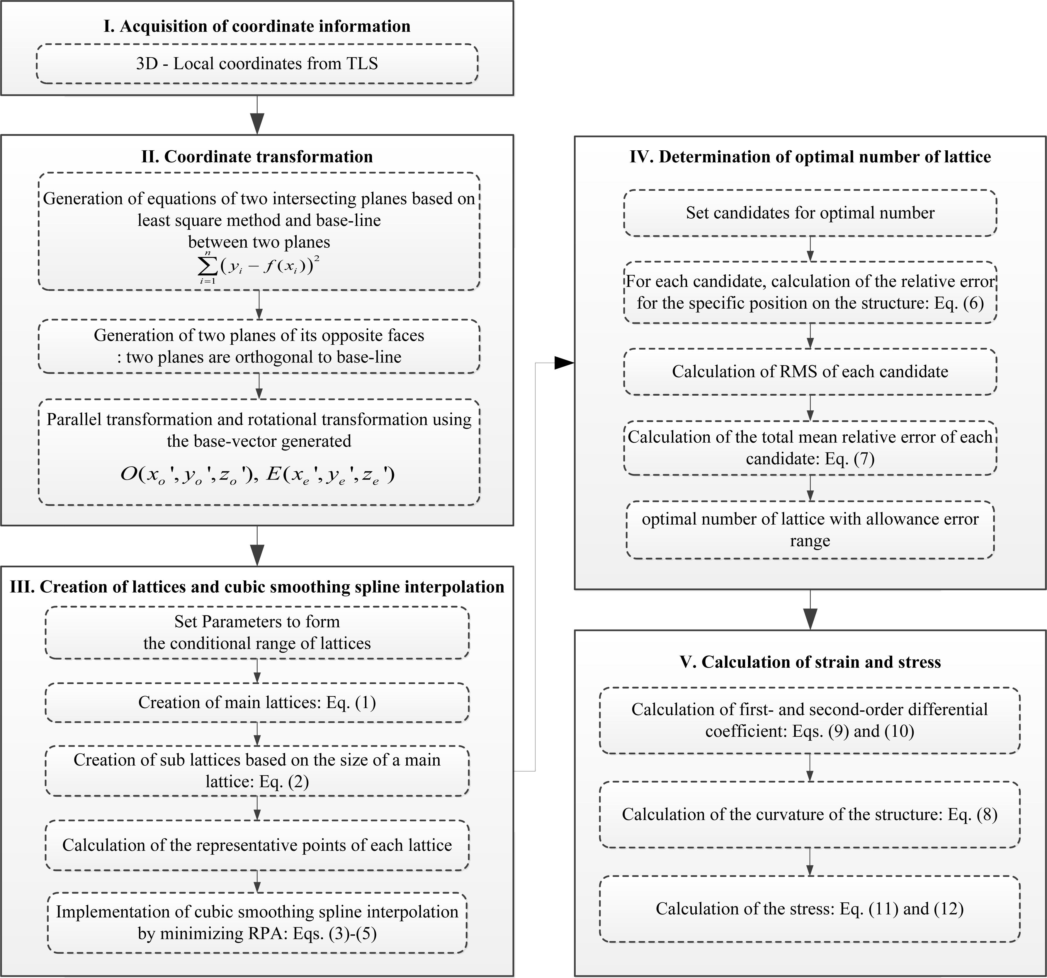

Light detection and ranging (LIDAR) has been introduced as a new vision-based monitoring method in the field of construction and civil engineering since the 2000s [1]. LIDAR is a noncontact measurement device that acquires 3D coordinates of objects using laser pulses, and was first introduced in geographic information systems [26]. Owing to its reliability, LIDAR is being used in various engineering fields [9, 17, 42, 51, 56]. LIDAR can be classified into airborne laser scanning (ALS) methods and terrestrial laser scanning (TLS) methods. The coordinate data for a target using laser scanning is acquired based on the time taken by numerous projected laser pulses that return post reflection or based on the phase difference between frequencies. The acquired coordinate data are used to express the shape of a target. The ALS method, which is based on remote measurement, cannot measure high-resolution data for structural modeling, but the TLS method can generate more accurate 3D coordinates and has numerous advantages such as noncontact measurement and minimal difficulty in measurement due to the surrounding environment. Thus, TLS is often used for health monitoring of structures such as buildings, tunnels, and bridges [14, 37].

Alba et al. conducted a strain measurement experiment for a large dam according to its water level height using a laser scanner [2]. In this study, they generated various datasets for point clouds through a mesh of point clouds, resampling, etc. and compared the measurement results. Park et al. suggested a model for estimating the displacement and deformed shapes of beam structures using TLS [36]. The maximum strain value estimated from the proposed model showed 1.6% or lower error rates. Lee and Park suggested a displacement estimation model that applied LSM to consider incorporating mutual deformation characteristics [20]. The model can calculate the coefficient of the polynomial shape function that minimizes the sum of squares of error vectors. Olsen et al. presented a structural damage assessment method using volumetric analysis and generated an average point by subdividing point clouds into 1 cm cubes to reduce noise [34]. Riveiro et al. conducted a limit analysis for masonry arch bridges by generating cubes and removing noises based on the octree structure [43]. However, their method requires multiple software applications; further, they did not present any clear standard for the number of divisions. A clear standard needs to be presented because estimated values can vary by the method of division and the characteristics of structure. Lee and Park suggested a stress distribution estimation model by applying FEM to compose a flexible matrix for the model presented in [21]. This estimation model requires the setting of point conditions and is limited to single shape functions for the most part. This limitation makes it difficult to estimate the stress distribution of a member on three dimensions and cannot be applied to members with large or non-uniform sections. Cabaleiro et al. suggested an algorithm to overcome the limitations of the current commercial software that can model standardized cross-sections of beams on condition that the structure in practice does not have an idealized straight line [5]. This algorithm needs a polynomial surface fitting process for the flange of the structure. If the resolution of TLS is not sufficient to measure the shape, a qualified application depending on the accuracy of the scanner would be required since the high range of error from 5 to 10 mm should be regarded. When there is a small deflection below 20 mm on the target, it may result in distorted information as torsion may occur on the beam with straight line even though there is no torsion on the surface of it. Truong-Hong and Laefer proposed a method to estimate the vertical displacement of the structure using a “cell” based on the octree method [50]. However, this study recommends that the size of the cell needs to be determined below 20 mm. This criterion is for the empirical value extracted from one element. In other words, the size of a cell for estimating the deformed shape could be changed according to the scale or shape of the structure. Thus, a definite method to determine the size of the cell is required. Furthermore, sensors using laser pulses such as TLS have a major problem with irregular distribution patterns of acquired points. This means that they cannot avoid a certain level of error because an even number of points are not present at the specified places. From this point of view, to utilize point clouds from TLS adequately, problems related to the occurrence of error points and differences in accuracy depending on the specification of the scanner need to be considered.

The main purpose of this study is to suggest a safety assessment method for a beam structure by using TLS. Unlike existing studies that focused on suggesting an accurate assessment method for the deformed shape of a beam structure by using TLS, this study proposed a safety assessment model that improves the continuity of curvature that constitutes second-order information on the deformed shape by generating double-layer lattices. Therefore, it can perform the safety assessment of a beam through a reliable assessment process by mitigating problems of TLS data to measure a deformation. In this progress, the number of lattices that can present the most similar shape of the actual target is suggested and CSSI using a third-degree polynomial is applied for the minimization of the distortion of the curvature by error points inevitably occurred in measurement process.

Figure 2.

Concept of the proposed model.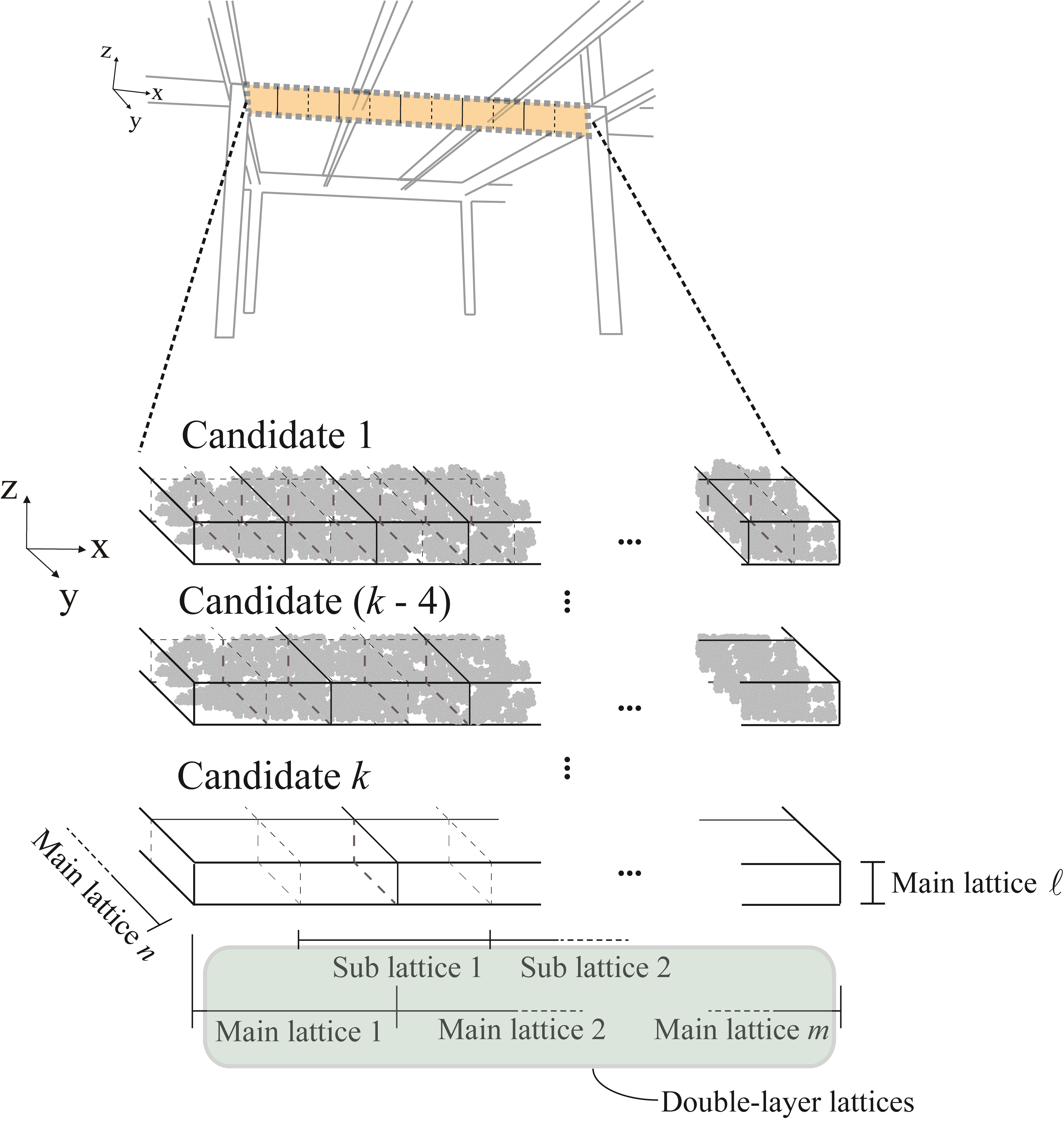

2. Stress estimation model

2.1 Algorithm

The algorithm of the stress estimation model proposed in this study consists of five steps as shown in Fig. 1: 1) Acquisition of 3D coordinate information through TLS, 2) Data coordinate transformation, 3) Creation of double-layer lattices and the application of CSSI, 4) Selection of the optimal number of lattices, and 5) Calculation of the strain on the structure.

In the first and second steps, flange and web can be separated from the beam point cloud manually using data processing software or automatically using commercial software such as Leica cyclone [24]. Based on the data acquired in the first and second steps, double-layer lattices are created and the CSSI method is applied to minimize curvature distortion in the third step. These double-layer lattices consist of main and sub lattices. To determine the optimal number of lattices, the numbers of lattices in the x-, y-, and z-axis directions ( $\ell$ , $m$ , $n$ ) are set as parameters. The optimal number is determined from the $k$ candidates for $\ell$ , $m$ , and $n$ as shown in Fig. 2. The representative point of each lattice is determined by calculating the average of points in each lattice and interpolation is conducted for the representative points. In the fourth step, the optimal number of lattice is selected using the root mean square (RMS). The candidate that meets the allowance error range set through repeated calculations is selected as the optimal number. In the fifth step, the curvature is determined and the stress is calculated by numerical differentiation of the deformed shape information based on the optimal lattice.

Figure 3.

The deformed shape of the upper flange of a steel beam obtained from TLS.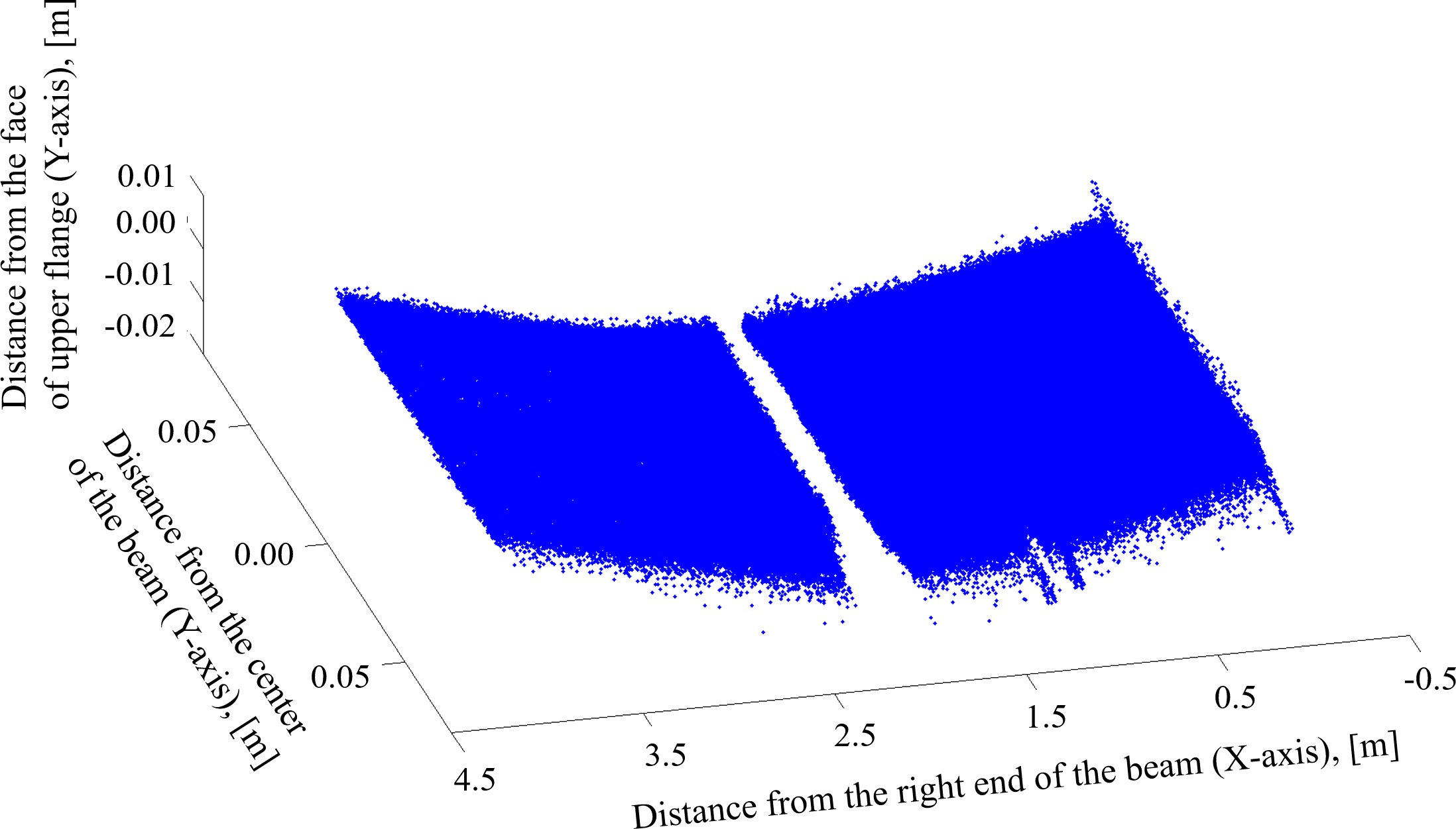

Figure 4.

Coordinate transformation of TLS data.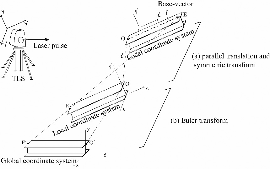

2.2 Acquisition of 3D coordinate information and coordinate transformation

In the first step, the 3D coordinate information of the target structure is obtained using TLS. For measurement, the location of the scanner, measurement angle, and scanning range are set in line with the measurement environment. TLS uses a high scan rate of over 50,000 points/s for more accurate and detailed expression of the target shape [11, 53]. Here, the set of numerous points having 3D coordinates obtained from TLS are usually referred to as “point cloud”. Figure 3 shows the shape of the upper flange of a steel beam that has a strain caused by external force. The empty space in the center of the shape resulted from the omission of measurement by a loading device.

As shown in Fig. 4, the 3D coordinate information by TLS is based on the local coordinates determined by the position and angle of TLS. To estimate the displacement or deformed shape of a structure, the local coordinates based on TLS need to be transformed to global coordinates based on the shape of the structure. To perform the transformation of the TLS coordinate system to the structure coordinate system, a base-vector for point clouds needs to be determined. The determination of a base-vector begins from the formation of an equation of planes for the flange and web faces based on the method of least square [20]. As the flange and web faces of the steel beam area contact each other, the equation of intersection can be derived from the equation of two planes as shown in Fig. 4a. A new equation of two planes is created that passes through the selected two points corresponding to the both ends of the flange and is orthogonal to the equation of intersection. The crossing point between the equation of planes and the equation of intersection generates a base-vector consisting of $O(x_{o}^{\prime},{\rm}y_{o}^{\prime},z_{o}^{\prime})$ and $E(x_{e}^{\prime},{\rm}y_{e}^{\prime},z_{e}^{\prime})$ as shown in Fig. 4a. By using the base-vector, the local coordinate information is transformed into global coordinate information as shown in Fig. 4a and b.

2.3 Creation of double-layer lattices

The displacement of a structure can be calculated by the variation between the coordinate information of load application and the coordinate information before the load application. To quantitatively determine this variation, representative points must be created to calculate the displacement of each part of the point cloud. As the first step to create representative points, lattices are created to divide the point clouds in uniform intervals. In this study, single lattices are defined as single segments with uniform intervals in the longitudinal direction of the target structure as shown in Fig. 5.

In this study, the lattice type is presented as double-layer lattices. These double-layer lattices are largely divided into main and sub lattices. Main lattices refer to those created first for the point cloud. Sub lattices are secondary lattices created to obtain continuity between main lattices. Because the points comprising a point cloud are irregularly distributed, they are likely to be concentrated in specific positions depending on the measuring position and angle. In particular, as the total number of points created at the time of measurement is constant, the number of points distributed in the unit lattice is inversely proportional to total number of the generated lattice $m$ . Therefore, some lattices may have very small or no points if the lattices are created in dense intervals. Therefore, increasing the number of main lattices with no specific ground cannot guarantee the minimization of error rate between the estimated value and the actual value. On the other hand, creating lattices with broad intervals increases the number of points in each lattice, and this makes it difficult to estimate the local deformations of the target structure. The concept of sub lattice was introduced in this study to solve this contradictory problem.

Figure 5.

Creation of lattices.

Figure 6.

Main and sub layer lattices for stress estimation model.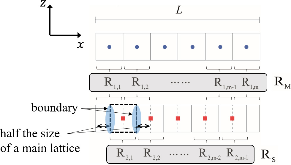

2.3.1 Main lattices and sub lattices

Figure 6 shows the lattices of a target structure with a length of $L$ and the creation process of main lattices and sub lattices. The $i$ th main lattice is created in the constraint range ${R}_{1,i}$ as shown in Eq. (1). ${R}_{M}$ is the total set of main lattices, and each of the constraint ranges ${R}_{1,1},{R}_{1,2},\ldots,{R}_{1,m-1},{R}_{1,m}$ is a partial set of ${R}_{M}$ . In Eq. (2.3.1), $j$ denotes the sub lattice number that should be generated. According to the correlation between Eqs (1) and (2.3.1), $(m-1)$ sub lattices are created when $m$ main lattices are created. ${R}_{S}$ denotes the total set of sub lattices, and ${R}_{2,1},{R}_{2,2},\ldots,{R}_{2,m-1}$ denote the partial sets of ${R}_{S}$ . To create sub lattice, the size of main lattice should be determined as mentioned. This is because the starting boundary of the sub lattice ${R}_{2,1}$ corresponds to the middle point of the adjacent main lattice, ${R}_{1,1}$ , and its ending point corresponds to the middle point of the other adjacent main lattice, ${R}_{1,2}$ . In other words, the starting and ending boundaries of the unit sub lattice corresponds to the middle point of each adjacent main lattice. Equation (2.3.1) explains this process to form sub lattices. After setting the size of the lattice, the representative points are determined through the calculation of the average of the points belonging to it, which are depicted as the circle markers with blue and square markers with red in Fig. 6.

$\displaystyle\frac{i-1}{m}L\leqslant{R}_{1,i}<\frac{i}{m}L\ldots({i=1,2,3,∼{}% \ldots∼{},m})$ (1) $\displaystyle\frac{2({j-1})-1}{2({m-1})}L\leqslant{R}_{2,j}<\frac{2({j-1})+1}{% 2({m-1})}L$ $\displaystyle\ldots\,\,({j=1,2,3,\ldots,m-1})$ (2)

The point cloud obtained from TLS is difficult to meet the compatibility condition because it has the characteristic of discrete distribution. Sub lattices induce continuous distribution by considering incorporating mutual deformation characteristics, and this can prevent discontinuous distribution of stresses by measurement errors among the adjacent measurement points in the assessment of the stress of a member. Furthermore, many points near the boundary line shared by two main lattices have similar coordinate data, but two points $(x_{1},y_{1},z_{1})$ and $(x_{2},y_{2},z_{2})$ in Fig. 7 belong to different lattices even though they have similar coordinate data. In this case, distorted deformations could appear because the correlations between points separated by the boundary line are not considered, and this can lead to sharp variations of stress distribution or curvature distortion at the boundary of lattices. This problem can be solved by applying sub lattices into data selection with main lattice whose concept such as cell or other forms is used in the previous studies on TLS, and the validity of double-layer lattices is verified through experimentation in Section 3.

Figure 7.

Boundary line between two main layer lattices.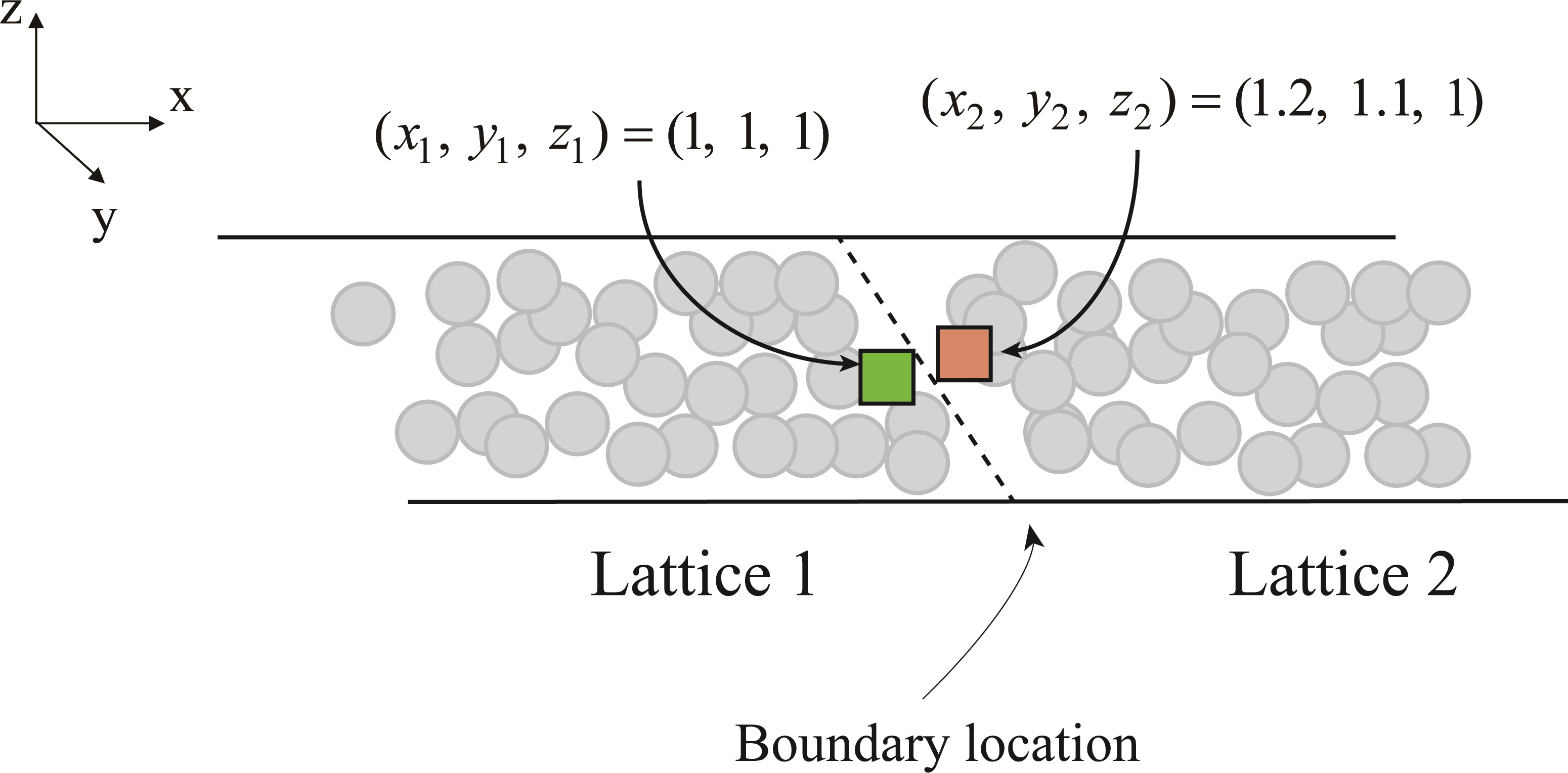

2.3.2 Expansion of lattices for multi-axis

Section 2.3.1 presented the concept of the lattice creation method for one axis direction. Lattices can be created in multi-axes instead of the single-axis direction. For structures such as bridges with huge dimension or girders of steel structures subjected to huge loads vertically, there is a need to consider the occurrence of torsion by various load pattern. Cabaleiro et al. pointed out that various type of deformations including torsion should be considered to estimate the realistic deformed shape of a beam [5]. Along these lines, the expansion of generating lattices to multi-axes is required to detect the irregular deflection on a plane. Figure 8 shows the lattices created in two axis directions of x and y axes based on the global coordinates. Figure 9 shows lattices created in the three axis directions.

Figure 8.

Creation of lattices in two directions.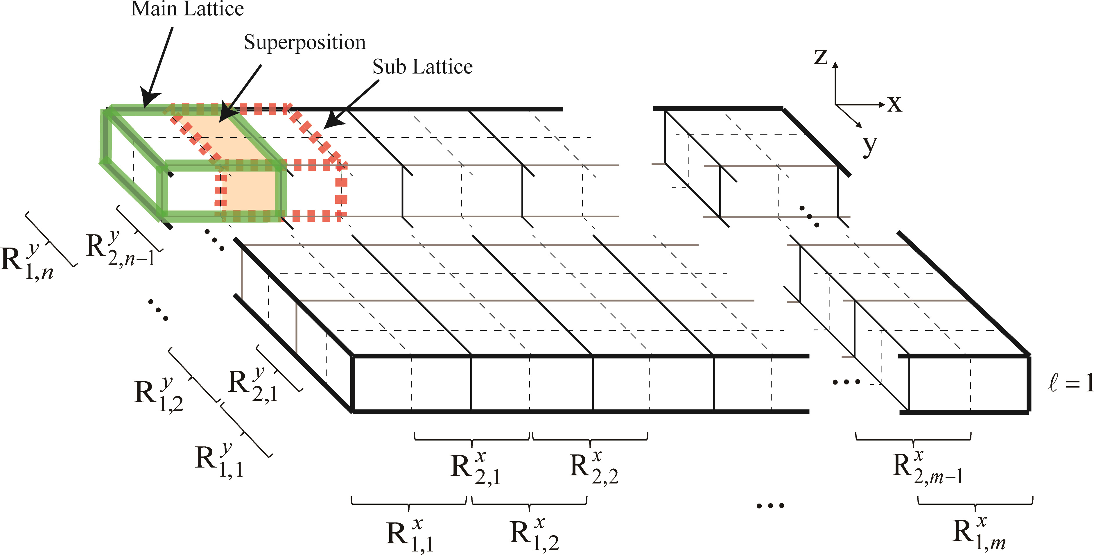

Figure 9.

Creation of lattices in three directions.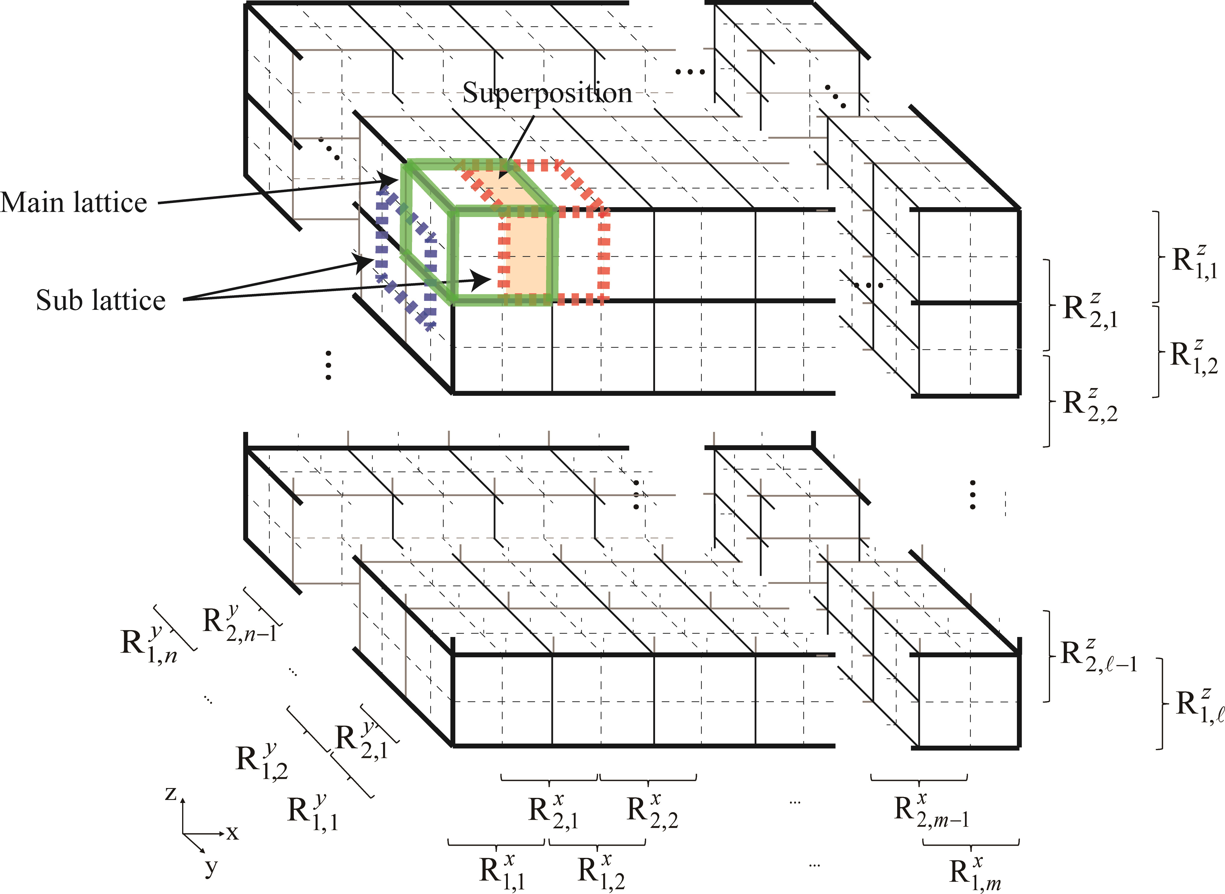

In Figs 7 and 8, superposition sections are generated by the creation of sub lattices between two main lattices. When there are $m$ main lattices in the $x$ -axis direction, $(m-1)$ sub lattices are generated. When the number of main lattices is $n$ and $\ell$ in the $y$ - and $z$ -axis directions, respectively, $(n-1)$ and $(\ell-1)$ sub lattices are generated. Therefore, the total number of lattices in three directions can be expressed as $({2m-1})\times({2n-1})\times(2\ell-1)$ .

2.4 Application of CSSI (Cubic smoothing spline interpolation)

Commercialized TLS devices in general provide a series of software applications in accordance with the purpose of users and include a post-processing feature for removing surrounding noises and obstacles. Depending on the case, the post-processed data may contain points that can affect noise or deformed shapes that have not been recognized. Because the measurement and post-processing step may contain unintended variables that affect analysis, a method of minimizing the potential error rate of estimated values needs to be considered.

CSSI is an interpolation method that estimates the deformed shape of structures in each section $[a$ $,$ $t_{1}$ $]$ $,$ $[t_{1}$ $,$ $t_{2}]$ $,$ $\ldots$ $,$ $[t_{n},b]$ having a distribution form with equal or unequal intervals for the total section $[a,b]$ in the $x$ -axis direction on two dimensions. The polynomial function determined using CSSI represents a shape function for vertical deflection (z-direction) of a structure.

$\displaystyle S(x)=d_{i}x^{3}+c_{i}x^{2}+b_{i}x+a_{i},x\in[r_{i},r_{i+1}]$ (3)

The third-degree polynomial applied to CSSI as shown in Eq. (3) is used to overcome the limitation of straight interpolation or to improve the efficiency in the calculation cost and accuracy of the interpolation process for high-degree polynomials [13]. In this third-degree polynomial, $a_{i}$ , $b_{i}$ , $c_{i}$ , and $d_{i}$ are the coefficients of the polynomial function $S(x)$ , where $i=0,1,\ldots,2m-1$ , and $m$ is the number of main lattices in the $x$ -axis direction; $r_{i}$ denotes the position of the $i$ th representative point of lattice, and $x$ represents a random point in the range of $[r_{i},r_{i+1}]$ . As shown in Eq. (2.4), the polynomial function $S(x)$ determines the constant of the function that minimizes its value using the roughness penalty approach (RPA) or regularization to set the optimum smoothness as shown in the following equation [15]:

$\displaystyle\textit{RPA}(S,\lambda)=\sum\limits_{i=1}^{n}{[f(x_{i})-S(x_{i})]% ^{2}}$ $\displaystyle+\lambda\int_{a}^{b}{[{S}^{\prime\prime}(x_{i})]^{2}dx}$ (4)

where $\sum\nolimits_{i=1}^{n}{[y_{i}-S(x_{i})]^{2}}$ is the square error between the measured value such as the vertical deflection and the third-degree polynomial and implies the compatibility between the two variables; $f(x_{i})$ represents the deflection amount for a random point $x_{i}$ of the structure; $\lambda\int_{a}^{b}{[{S}^{\prime\prime}(x)]^{2}dx}$ represents the roughness of data; and $\lambda$ denotes the smoothness parameter. The data smoothness varies by $\lambda$ and the application of an inappropriate value can distort the shape. The calculation of an appropriate $\lambda$ can be done by applying cross-validation, which is a representative accuracy assessment method for an approximate model as shown in the following Eq. (5) [15]:

$\displaystyle\min\textit{CV}(\lambda)=\frac{1}{n}\sum\limits_{i=1}^{n}{[f(x_{i% })-\hat{{S}}^{(-i)}(x_{i})]^{2}}$ (5)

where $\hat{{S}}(x_{i})$ represents the estimated smoothness curve and plays the role of a prediction variable to find the optimum $\lambda$ . The $\lambda$ determined through cross-validation is applied to Eq. (2.4), and the polynomial $S(x)$ that has the lowest RPA is selected.

As mentioned in Section 2.3, the number of lattices needs to be restricted. Because the data acquired by TLS is discretely distributed, it is difficult to estimate the stress distribution for a random point of a target structure. Therefore, the application of CSSI enables the deduction of the function value for a random point while generating a shape function of the third-degree polynomial, and this enables the estimation of the global stress distribution of a structure or member.

2.5 Optimal number of lattice

The representative point of each lattice are used when estimating the shape function based on 3D data acquired through measurement. Thus, the number of lattices that can minimize the distortion of the deformed shape needs to be set. The number of lattices varies by the size of the target structure, sampling rate, etc. An efficient method that enables quantitative evaluation is required to determine the optimal number of lattices for each target structure. This section describes this process.

Figure 10.

RMS of a population to select the optimal number of lattice.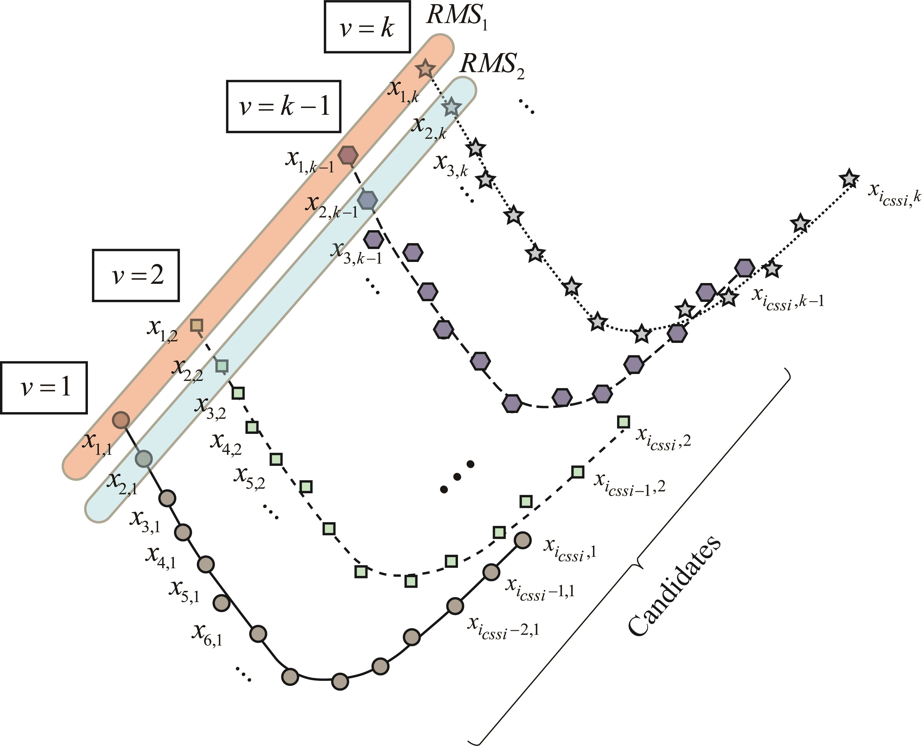

As mentioned in Section 2.3.1, the range of each lattice is defined by Eq. (1) and the total number of lattices of the structure is determined by this range. The number of points in a lattice is inversely proportional to the values of $\ell$ , $m$ , and $n$ . The value of the representative point of each lattice is determined by the coordinates of the measurement points, and this is used to estimate the deformed shape of the target. Equation (6) shows the relative error equation for the specific position of each candidate.

$\displaystyle\textit{RE}_{S,v}=\frac{|{({|{f(x_{S,v})}|-\textit{RMS}_{S}})}|}{% \textit{RMS}_{S}}$ (6)

$\textit{RE}_{S,v}$ denotes the relative error between the function value at the $S$ th position of the $v$ th candidate and the $\textit{RMS}_{S}$ . $\textit{RMS}_{S}$ denotes the root mean square of each candidate at the $S$ th position. Candidates here refer to the cases that have the possibility of becoming the optimal number of lattices. Figure 10 shows the creation method of the optimal number of lattices based on RMS. In Fig. 10 and Eq. (6), $v$ is $1,2,\ldots,k-1,k$ , and $k$ is the total number of candidates for the calculation of optimal number of lattice. $i_{cssi}$ denotes the number of the interpolated data. $x_{S,v}$ denotes the $S$ th position among $i_{cssi}$ for the $v$ th candidate. The total mean relative error rate $f_{v}$ of each candidate can be determined by calculating the square means of the function values for the section from 1 to $i_{cssi}$ with the following Eq. (7):

$\displaystyle f_{v}(C,S,r)=\sqrt{\frac{\sum\limits_{S=1}^{p}{(\textit{RE}_{S,v% })^{2}}}{i_{cssi}}}<\varepsilon_{r}$ (7)

where $C$ denotes the interpolated data by CSSI, $\varepsilon_{r}$ denotes the allowance error range, $r$ denotes the repeated calculation count. Candidates that do not meet $\varepsilon_{r}$ are dropped and the process of Eqs (6) and (7) is repeated $r$ times until a single candidate is selected. $\varepsilon_{r}$ has a similar concept for margin of error expressed as a product of a threshold value and a standard error from a statistical perspective. In this study, the set of the threshold value is based on $\sum\nolimits_{S=1}^{p}{\textit{RE}_{S,v}}$ according to the number of double lattices, and the standard error can be calculated by the square root of the value that is a sample variance for the number of candidates. Finally, the optimal solution provides two options because the application of Eqs (6) and (7) is not suitable for the two short-listed candidates.

Figure 11.

Deformed shape of a beam for external force.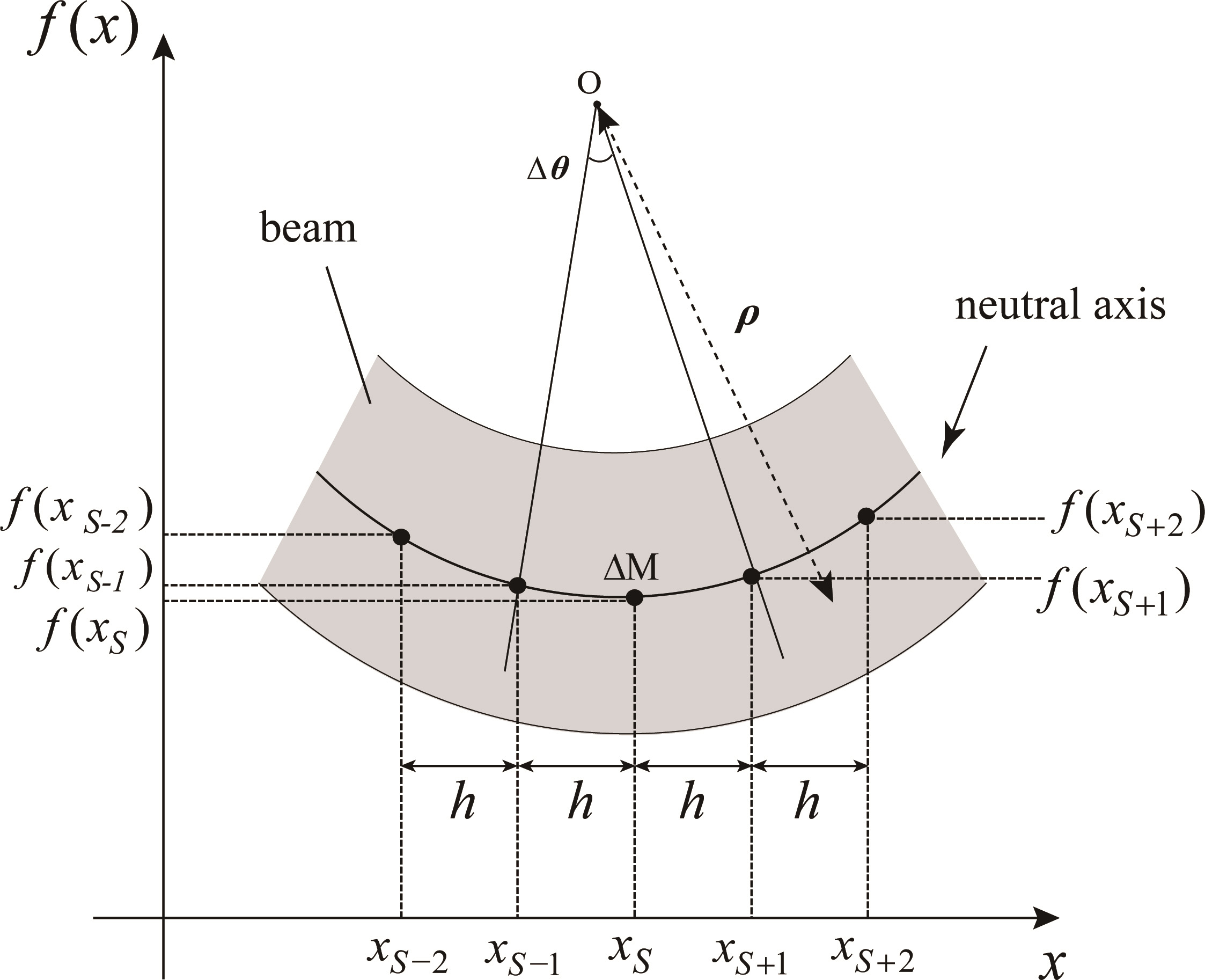

2.6 Evaluation of stress

The calculation of the stress occurring in a structure is based on the Euler-Bernoulli beam theory that a plane perpendicular to the neutral plane always maintains a perpendicular state, and Hooke’s Law [12]. Since it is difficult to obtain the shape of a perfect line from a beam even if it is processed accurately without any error or damage, thessumption that the initial condition of beam is an idealized straight line is considered in the model.

Figure 12.

Specimen for experimental verification of the proposed model.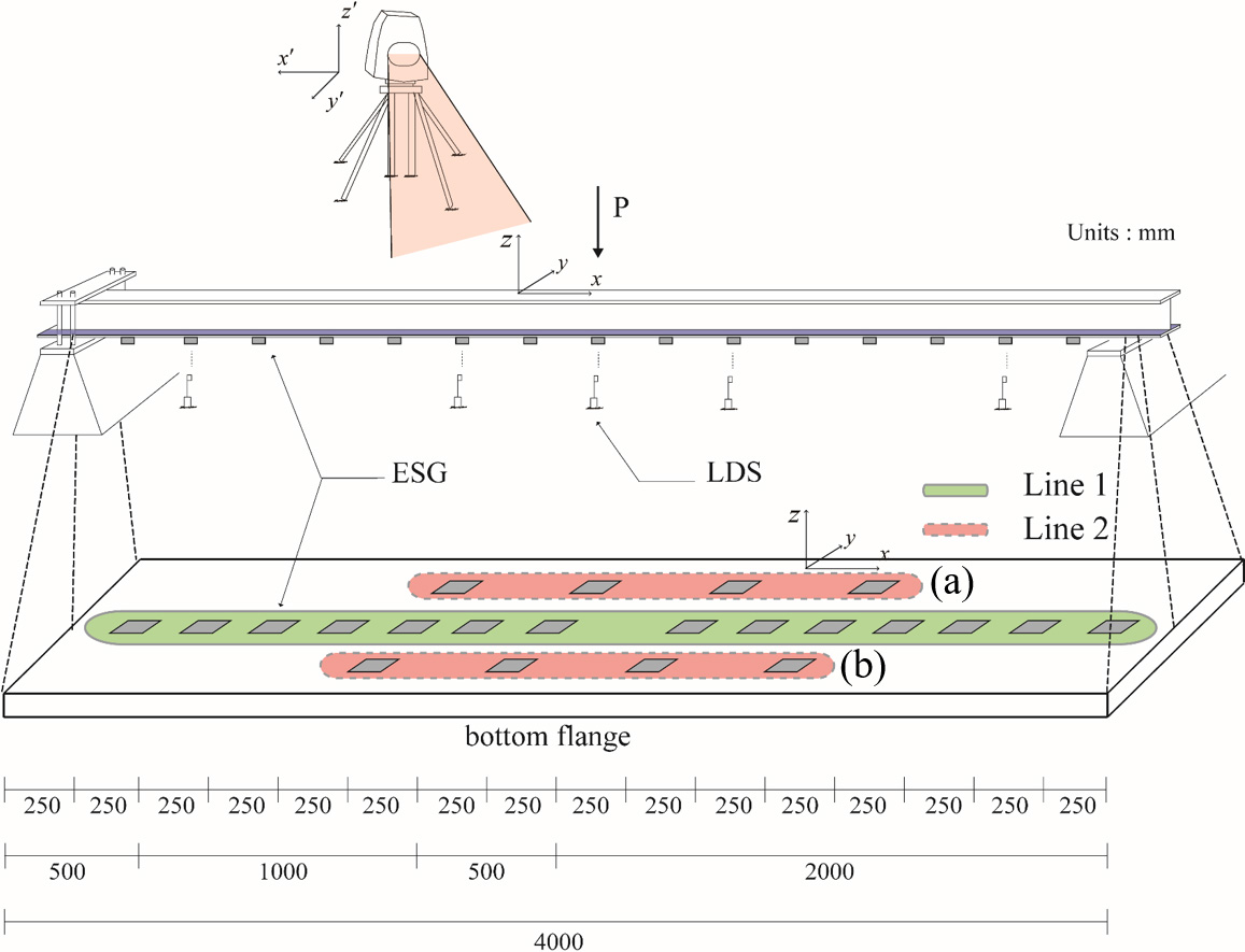

Figure 13.

Photograph of the experimental measurement using TLS.

The strain that occurs at each point in a structure can be calculated through the differential coefficient that signifies the slope of the function between points. Figure 11 shows the deflection of the beam under the influence of top load.

$\displaystyle K_{S}=\frac{1}{\rho}=\frac{d\theta_{S}}{dM_{S}}=\frac{{% \displaystyle\frac{d^{2}f(x_{S})}{dx_{S}^{2}}}}{\left[{1+\left({{\displaystyle% \frac{df(x_{S})}{dx_{S}}}}\right)^{2}}\right]^{\frac{3}{2}}}$ (8)

Equation (8) is an expression of the curvature for the $S$ th position $K_{s}$ by $x_{S}$ and the function value $f(x_{s})$ . The curvature $K_{s}$ is based on each $\Delta\theta$ that is determined by the minute movement distance $\Delta M$ from point $P$ to point $Q$ and the tangent for each point. $x_{s}$ denotes the random point in the longitudinal direction of the beam, and $\rho$ denotes the radius of curvature. $h$ denotes the distance between points and when this distance is narrower, the accuracy becomes higher.

$\displaystyle\frac{df(x_{S})}{dx_{S}}=\frac{f(x_{S-2})-8f(x_{S-1})}{12∼{}h}$ $\displaystyle\quad∼{}+\frac{8f(x_{S+1})-f(x_{S+2})}{12∼{}h}$ (9) $\displaystyle\frac{d^{2}f(x_{S})}{dx_{S}^{2}}=\frac{-f(x_{S-2}){+}16f(x_{S-1})% {-}30f(x_{S})}{12h^{2}}$ $\displaystyle\quad∼{}+\frac{16f(x_{S+1})-f(x_{S+2})}{12∼{}h^{2}}$ (10)

Equations (2.6) and (2.6) represent the expressions for the first and second derivatives, respectively. Four-point central difference and five-point central difference were used to determine first and second derivatives, respectively. The strain can be calculated by multiplying curvature $K_{S}$ by the distance $d$ from the neutral axis. This is expressed by the following Eq. (11):

$\displaystyle\varepsilon_{S}=K_{S}\cdot d$ (11) $\displaystyle\sigma_{S}=E\cdot\varepsilon_{S}$ (12)

Table 1

Optimal number of lattices, the number of repetition and allowance error range

Displacement control	The number of lattices			Optimal number of lattices	The number of repetition	$\varepsilon_{r}$
	X-axis	Y-axis (fixed)	Z-axis (fixed)
Step 1 (Initial)	–	–	–	–	–	–
Step 2 (10 mm)	77 (101)	3	1	291 (303)	113	3.7%
Step 3 (15 mm)	75 (201)	3	1	225 (603)	47	0.7%
Step 4 (20 mm)	48 (104)	3	1	144 (312)	43	1.4%

where $\varepsilon_{S}$ denotes the strain at the $S$ th position of the beam. Equation (12) can calculate the stress $\sigma_{S}$ using $\varepsilon_{S}$ . The elastic coefficient $E$ of the steel beam is assumed to be a constant value.

Table 2

Relative error between TLS and LDS for estimated displacement

Displacement control	Distance from the left and of the beam (m)	Displacement estimated by TLS (m)	Displacement measured by LDS (m)	Relative error (%)
Step 1 (0 mm)	Initial state
Step 2 (10 mm)	0.5	$-$ 0.0038	$-$ 0.0038	$-$ 0.04
	1.5	$-$ 0.0089	$-$ 0.0087	1.97
	2.0	$-$ 0.0097	$-$ 0.0092	4.99
	2.5	$-$ 0.0089	$-$ 0.0089	$-$ 0.63
	3.5	$-$ 0.0035	$-$ 0.0039	$-$ 10.24
Step 3 (15 mm)	0.5	$-$ 0.0061	$-$ 0.0041	46.54
	1.5	$-$ 0.0132	$-$ 0.0123	7.52
	2.0	$-$ 0.0142	$-$ 0.0138	2.99
	2.5	$-$ 0.0130	$-$ 0.0127	2.26
	3.5	$-$ 0.0054	$-$ 0.0055	$-$ 1.65
Step 4 (20 mm)	0.5	$-$ 0.0080	$-$ 0.0066	22.16
	1.5	$-$ 0.0174	$-$ 0.0176	$-$ 1.41
	2.0	$-$ 0.0186	$-$ 0.0186	$-$ 0.07
	2.5	$-$ 0.0169	$-$ 0.0170	$-$ 0.32
	3.5	$-$ 0.0068	$-$ 0.0071	$-$ 3.98

Figure 14.

Estimation deformed shape.

3. Experiment

Steel beam loading experiments were conducted to validate the proposed model. Figures 12 and 13 show the measurement experiments conducted for the verification of the proposed model using the specimen and TLS. For the target specimen, SS400 grade steel with a 4-m long section of ${H}-100\times 100\times 6\times 8$ , an elastic coefficient of 206 GPa, and yield strength of 235 MPa were selected. One ScanStation C10 from Leica was used for the TLS model; this scanner can measure a target up to 360 ${}^{\circ}$ and 270 ${}^{\circ}$ in the horizontal and vertical directions, respectively. It has an accuracy of 6 mm and 4 mm for position and distance, respectively. In addition, the scan rate can be set up to 50,000 points/s within a distance of 300 m [11]. The scanner was installed at a maximum distance of 4.3 m from a beam end. The incident angle was between 0 ${}^{\circ}$ and 55 ${}^{\circ}$ and the scan rate of the sensor was set up to 1000 points/s, and these factors can affect the interval between points that constituted point clouds or the occurrence of noise data [47]. The laser displacement sensor (LDS) used to compare the reliability of TLS measurement data was the LB-301/LB-1201 (Sensor head/Controller, Keyence) model with a display resolution of 50 $\mu m$ and measuring distance of 300 mm ( $\pm$ 100 mm) [44]. Five LDSs were used and they were positioned at 0.5, 1.5, 2.0, 2.5, and 3.5 m on Line 1 as shown in Fig. 12. An ESG was used as the sensor for the verification of the estimated stress distribution. To derive the result of the stress distribution estimation on a plane for comparison, ESGs were attached longitudinally in three lines on the bottom flange of the steel beam as shown in Fig. 12.

Figure 15.

Differential coefficient of estimated shape function.

Figure 16.

Distribution of estimated stress for each step (displacement control: 10mm, 15mm and 20mm).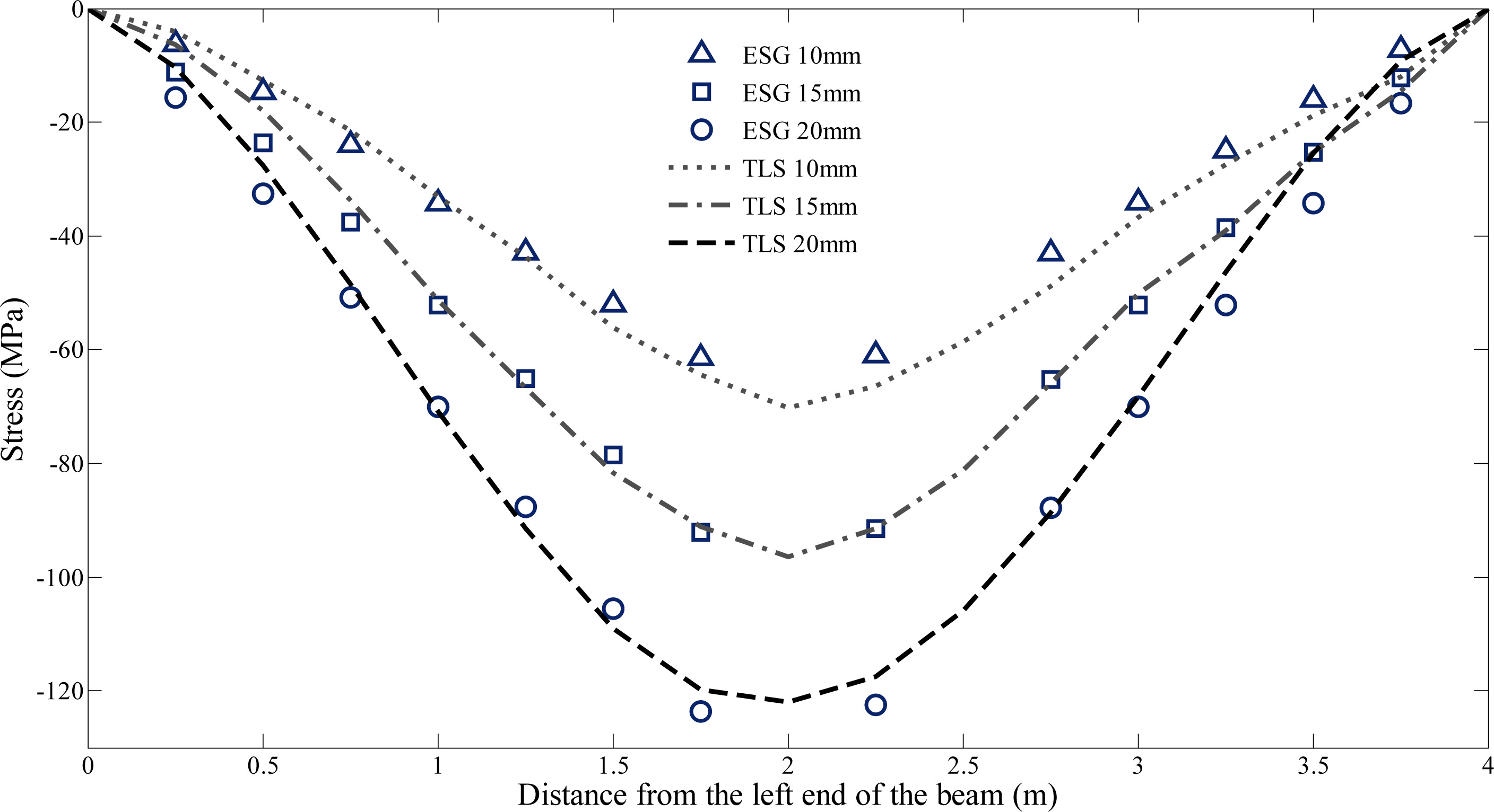

On Line 1, which represents the center line, 14 ESGs were attached in 0.25 m intervals. For Line 2 representing left and right lines, four ESGs were attached at intervals of 0.5 m. A hydrodynamic actuator that can control displacement was used to apply load to the structure. For displacement control, a loading experiment was conducted for four steps including the initial test, 10 mm, 15 mm, and 20 mm. The z axis was fixed as a single lattice to facilitate the verification of the method and a conditional range was applied to the $x$ and $y$ axes directions based on Eqs (1) and (2.3.1). The point cloud of the beam was extracted from all obtained TLS data through the data processing software related to the sensor. As the cross-section of the beam was relatively small and standardized, the data of the beam could be obtained manually by eliminating the points around the target. In addition, the mixed pixels around the edge of the beam were manually eliminated by the user.

4. Result

4.1 Response estimation

The optimal number of lattices for each step (displacement control: 0 mm, 10 mm, 15 mm, and 20 mm, respectively) selected as shown in Table 1 using the method described in Section 2.5. In Table 1, the X-axis represents the longitudinal direction of the flange as shown in Fig. 13, the Y-axis represents the number of lattices in the width direction of the flange, and the Z-axis represents the number of lattices in the depth direction of the flange. Unlike the case of creating lattices in the single-axis direction, the creation of lattices in the multi-axes estimates the deformed shape on the plane. To verify the result value of the estimation model, the total number of lattices for the Y-axis was fixed at 3 and it was compared with ESGs attached in three lines along the X-axis. The number of lattices in the Z-axis was fixed at 1 to facilitate the verification. The size of lattices were considered up to 12 times smaller than the optimal candidate.

Table 3
Relative error between TLS and ESG for estimated stress distribution (displacement control: 10 mm)

Distance from the left and of the beam (m)	Stress estimated by TLS (MPa)	Stress estimated by ESG (MPa)	Relative error (%)
0.25	4.10	6.28	34.71
0.50	12.63	14.63	13.72
0.75	21.45	23.99	10.56
1.00	33.15	34.23	3.14
1.25	43.72	42.84	2.06
1.50	56.10	52.03	7.83
1.75	64.38	61.40	4.85
2.25	66.37	60.89	9.00
2.75	48.77	43.05	13.30
3.00	36.68	34.07	7.66
3.25	27.36	24.97	9.59
3.50	18.83	15.92	18.25

Table 4

Relative error between TLS and ESG for estimated stress distribution (displacement control: 15 mm)

Distance from the left and of the beam (m)	Stress estimated by TLS (MPa)	Stress estimated by ESG (MPa)	Relative error (%)
0.25	6.36	11.23	43.35
0.50	17.95	23.69	24.26
0.75	33.78	37.48	9.87
1.00	51.36	52.16	1.54
1.25	66.79	65.07	2.64
1.50	81.73	78.51	4.10
1.75	91.10	92.14	1.12
2.25	91.38	91.44	0.06
2.75	65.91	65.31	0.91
3.00	50.24	52.09	3.56
3.25	39.11	38.62	1.28
3.50	25.32	25.28	0.15

Table 5

Relative error between TLS and ESG for estimated stress distribution (displacement control: 20 mm)

Distance from the left and of the beam (m)	Stress estimated by TLS (MPa)	Stress estimated by ESG (MPa)	Relative error (%)
0.25	10.31	15.66	34.18
0.50	27.59	32.55	15.22
0.75	48.48	50.85	4.66
1.00	70.94	70.09	1.20
1.25	91.42	87.56	4.41
1.50	109.03	105.55	3.29
1.75	119.85	123.54	2.98
2.25	117.56	122.45	3.99
2.75	88.66	87.73	1.06
3.00	68.26	69.98	2.46
3.25	46.40	52.07	10.88
3.50	25.43	34.29	25.84

Table 6

Relative error between TLS and ESG for estimated stress distribution - Line 2

Displacement control		(a) Location (m)				(b) Location (m)
		1.25	1.75	2.25	2.75	1.25	1.75	2.25	2.75
Step 2	TLS	45.39	54.59	56.03	45.60	42.27	67.61	68.92	44.92
	ESG	42.31	59.77	89.75	42.94	43.70	62.23	62.42	44.79
	Relative error (%)	7.29	8.67	37.57	6.19	3.26	8.63	10.42	0.29
Step 3	TLS	75.87	84.28	78.18	60.76	66.85	95.88	97.29	66.95
	ESG	64.26	89.86	89.75	64.43	66.34	93.10	93.09	67.02
	Relative error (%)	18.07	6.21	12.90	5.69	0.77	2.98	4.51	0.11
Step 4	TLS	85.51	114.64	116.44	93.75	89.81	125.62	125.69	88.37
	ESG	86.31	120.75	120.65	86.34	89.24	124.39	124.82	89.76
	Relative error (%)	0.93	5.06	3.49	8.58	0.65	0.99	0.70	1.54

Figure 17.

Comparison of double-layer lattices with single layer lattices for the estimated stress distribution.

To find the optimal number of lattices, 15% as an initial allowance error range was set based on the margin of error for the confidence interval of 99%. The computational procedure was performed repetitively until the final candidate that met the prescribed allowance error range was obtained. As the number of candidates decreased, the sensitivity increased and the sample analysis tended to be limited. Thus, the allowance error range decreased by 0.1% sequentially from the initial value. As a result of the calculation of the optimal number of lattices, 77 and 101 lattices were determined for the X-axis in step 2 where 10 mm displacement control was applied. A total of 291 and 303 lattices were calculated and 113 calculations were repeated. The allowance error range $\varepsilon_{r}$ was 3.7%. In step 3, 225 and 603 lattices were selected through 47 repeated calculations. The $\varepsilon_{r}$ was 0.7% in this step. In step 4, 48 and 104 lattices for X-axis and a total of 144 and 312 lattices were selected through 43 repeated calculations. The $\varepsilon_{r}$ was 1.4% error in this step. The candidate with a smaller value than the other was considered as the main solution for each load step (step 1: 291, step 2: 225, step 3: 144).

Among the candidates excluded from the maximum 113 repeated calculations to determine the optimal number of lattices, the maximum $f_{v}$ (total mean relative error rate of each candidate) was 40% and the maximum $R E$ (error rate at each point) was 191.05%. In other words, because the randomly set number of lattices can cause an error in the safety evaluation, the optimal number of lattices corresponding to the measurements of a verified sensor is a required process. The displacement of the structure for Line 1 was estimated based on the optimal number of lattices. Table 2 shows the error rate between the estimated value based on the proposed method and the measurement through LDS. Here, step 1 represents the initial state that has no load. In step 2, relative errors of less than 5% occurred at all points except the 3.5 m point. In steps 3 and 4, relative errors of less than 8% and 5% occurred, respectively, in all sections except the 0.5 m point. The results of the estimation model generally show a similar pattern as that of the measurements of the reference sensor. A greater error rate occurs as it is closer to both ends of the structure, but the absolute values have a difference of less than 2 mm at the maximum. Figure 14 shows the estimated values based on the proposed model and the method of least square, and the measurements of LDS together. The dotted curve in Fig. 14 shows the de formed shape of the target structure that was calculated based on the CSSI. The shapes of trapezoid and small rectangular present the estimated value by Cubic and Quadratic polynomial, respectively. Each marker indicates the installed point of LDS. The estimated values from cubic and quadratic polynomial functions shows a maximum relative error of 13.04%, 7.25%, and 3.2% with the measured data for each load step, respectively. Thus, the proposed model, which includes the process of creation of double-layer lattices and the application of CSSI has relatively higher reliability than others.

4.2 Stress estimation

The target specimen has an elastic coefficient of 206 GPa in theory. Thus, the stress distribution was estimated in this study by setting the condition that all sections have a uniform elastic coefficient. For the specimen that is bent by external force, the curvature can be calculated on the basis of the first-order and second-order differential coefficients. Figure 15 shows the calculation results obtained by applying the estimated value for Line 1 to Eqs (2.6) and (2.6). In Fig. 15a, the differential coefficient becomes closer to 0 when it is closer to the center of the structure where the maximum stress occurs. Because the coefficients to the left of the central point of the structure are negative, the slope of the shape function can be expected to indicate the negative direction. In contrast, the slope of the shape function that appears in the right side can be expected to occur in the increasing direction. Meanwhile, Fig. 15b showing the trend of the second-order differential coefficient, the left side from the central point indicates a decreasing function. According to this trend, it can be expected that a shape function that is curving upward is generated in the left side and a shape function that is curving downward as an increasing function is generated in the right side.

Figure 16 shows the estimation result of stress distribution calculated through Eqs (11) and (12). The dotted line of each type in the graph represents the calculation result based on the proposed model, and each marker indicates the measurement of ESG, which is the reference sensor. The stress distribution form is similar to the shape inferred in Fig. 15. The quantitative values in Fig. 16 are listed in Tables 3–5, respectively. Each table also shows the relative error rate between the estimated and measured values.

Figure 18.

Shape of uniplanar stress distribution.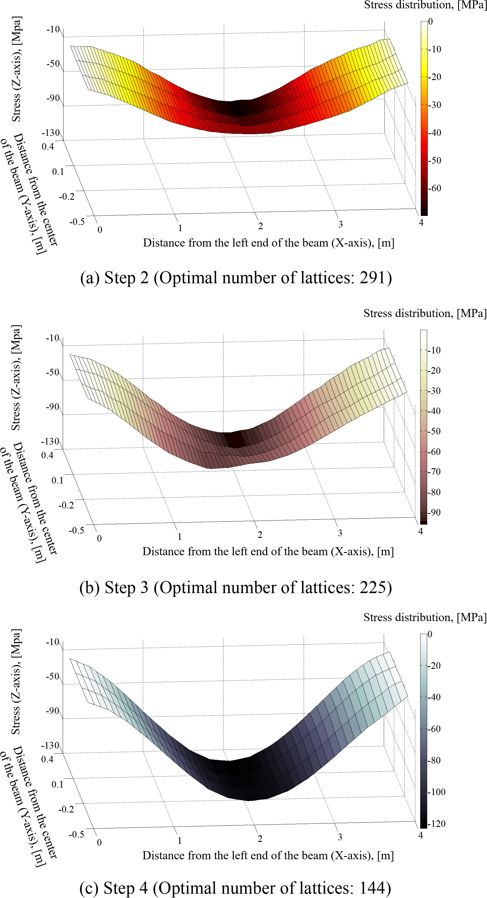

In Table 3, most of the estimated stress values in the section from 0.75 m to 3.25 m of the target structure show relative errors of less than 10%. In Table 4, all the values showed error rates of less than 5% except the section from 0.25 m to 0.75 m. In particular, the 1.75 m and 2.25 m points, where the maximum stress was expected, showed low relative error rates of 1.12% and 0.06%, respectively. Furthermore, in Table 5, the section from 0.75 m to 3.0 m showed error rates of less than 5%. The range of relative errors generated for each load step are different. This phenomenon results from the variation in the number of points in each lattice and the coordinate information owing to the difference in the distribution form of point cloud for each step conducted independently.

In Fig. 12, the ESG sensors attached on Line 1 belong to a major section of interest. On the other hand, Line 2 is divided into (a) and (b), which was used to verify the validity of the proposed method for the estimation of stress distribution on a plane. The results are listed in Table 6. Except for the measurement errors of the verification sensor at the 2.25 m point in (a), the mean error rates of the estimated values at other points showed values of 10.30%, 6.41%, and 2.74%, respectively, in each step. The error rate decreased as the displacement control increased. In particular, a high accuracy of less than 2% can be seen in line (b) of step 4. It shows that although the distance between line (a) and line (b) is about 100 mm, which is relatively short, ESG measurement values for the same point can be different. This phenomenon can occur adequately when the member section is large or in actual steel structures, and this demonstrates that the proposed method can estimate such stress distribution patterns.

The stress or strain at the ends that have a smaller value than the maximum strain are not used to evaluate the safety of structures, and large relative errors occur when the absolute value is small. On the other hand, the loading points where higher strain and stress occur need to be examined carefully in safety evaluation. Consequently, the proposed stress estimation model showed an error rate of less than 10% at the maximum stress point. This result supports the reliability of the proposed model and proves that the proposed model is appropriate for the estimation of stress on a plane.

Figure 17 compares the estimation results of stress distribution between double-layer lattices and single layer lattices to validate double-layer lattices. The two layer types show a common pattern in that the error rate decreases as the strain increases. However, the estimation accuracy of the stress distribution is lower when the single layer lattices are used. In particular, the error rate for the maximum stress point was higher than 9% when the stress distribution was estimated by applying single layer lattices, but the error rate was lower than 9% when double-layer lattices were applied. The results of this experiment and the application results of the method overcame the continuity limitation in Section 2.2 and verified the validity of double-layer lattices.

Figure 18 shows the stress distribution shape of the structure based on the optimal number of lattices suggested in Table 1. Figure 18a shows the displacement control experiment for 10 mm, and a total of 291 optimal lattices were generated to estimate the stress distribution shape. In Fig. 18b and c, 225 and 144 optimal lattices were calculated, respectively. The differences in the optimal number of lattices for step seem to be caused by the distribution pattern of point clouds that varies by the degree of displacement control and the wave characteristics of laser in each experimental step.

5. Conclusion

This study proposed a stress distribution estimation method for 3D structures using multi-dimensional double-layer lattices composed of main lattices with a specific constraint range and sub lattices that depend on the main lattices. Double-layer lattices were used to minimize the estimation error considering the distribution characteristics of acquired points. Further, the optimal number of lattices was determined using the RMS method. The representative points from each lattice were used to present the deformed shape of a target, and the curvature distortion that occurred owing to error points was minimized using CSSI. Based on the Euler–Bernoulli beam theory, the stress of the structure was calculated and its distribution was shown on a plane.

To verify the proposed model, 4-step displacement control experiments were conducted for 4-m long steel beams. As a result of three loading experiments, optimal lattices were determined for each step. The comparison of the measured and estimated values showed errors of less than 5% at the maximum displacement point. The measurement results verified the validity of the proposed stress distribution estimation method. In addition, double-layer lattices were more effective compared to single layer lattices in estimating the deformed shape. Furthermore, it was possible to estimate the stress distribution on a plane by expanding the generation of lattices to multiple-axes and the results obtained using ESGs exhibited allowable relative errors.

However, it should be noted that, as the displacement at the start of the beam is slightly less than zero as shown in Fig. 14, the relative error at this location is higher than those at other locations. There is a likelihood of the problem related to the technical limitation of TLS with accuracy of 6 mm for a single measurement and 2 mm for surface precision (noise). Thus, if TLS with improved accuracy for measuring the target is used for practical purposes, the boundary condition of the beam can be set in a better manner. Furthermore, adequate investigation of the surface state of the beam is required because the resolution of the point cloud and the measurement capacity of the scanner change with the reflectivity of materials. As the proposed model is for only elastic beam structures based on the Euler-Bernoulli beam theory, it is difficult to adopt the model for other structural elements that should consider axial forces or other bending theories. It is also difficult to use the model for dynamic analysis in practice since TLS does not scan the target structure in a frame simultaneously. Nevertheless, if users have information about the elastic modulus of materials, this model can be applied to any element regardless of the type of material for the direction of gravity. This is because TLS provides point clouds for the shape of the target based on the 3D coordinate system.

Footnotes

Acknowledgments

This work was supported by a National Research Foundation of Korea (NRF) grant funded by the Korea government (MSIP) (No. 2011-0018360).

References

Ackermann

. Airborne laser scanning – present status and future expectations. ISPRS Journal of Photogrammetry and Remote Sensing 1999; 54(2): 64-67.

Alba

Fregonese

Prandi

Scaioni

Valgoi

. Structural monitoring of a large dam by terrestrial laser scanning. International Archives of Photogrammetry, Remote Sensing and Spatial Information Sciences 2006; 36(5): 6.

Amezquita-Sanchez

Adeli

. Synchrosqueezed wavelet transform-fractality model for locating, detecting, and quantifying damage in smart highrise building structures. Smart Materials and Structures 2015; 24(6): 065034.

Bhalla

Yang

Zhao

Soh

. Structural health monitoring of underground facilities–technological issues and challenges. Tunnelling and Underground Space Technology 2005; 20(5): 487-500.

Cabaleiro

Riveiro

Arias

Caamaño

. Algorithm for beam deformation modeling from LiDAR data. Measurement 2015; 76: 20-31.

Cha

Buyukozturk

. Structural damage detection using modal strain energy and hybrid multi-objective optimization. Computer-Aided Civil and Infrastructure Engineering 2015; 30(5): 347-358.

Cho

Spencer

. Sensor attitude correction of wireless sensor network for acceleration-based monitoring of civil structures. Computer-Aided Civil and Infrastructure Engineering 2015; 30(11): 859-871.

Committee

ACI

. Building code requirements for structural concrete (aci 318-08) and commentary. American Concrete Institute 2008.

Domínguez

Alonso

Onieva

González

. A transferable belief model applied to lidar perception for autonomous vehicles. Integrated Computer-Aided Engineering 2013; 20(3): 289-302.

10.

Fraser

Riedel

. Monitoring the thermal deformation of steel beams via vision metrology. ISPRS Journal of Photogrammetry and Remote Sensing 2000; 55(4): 268-276.

11.

Geosystems

. Leica ScanStation c10, Product Specifications: Heerbrugg, Switzerland. 2012.

12.

Gere

Timoshenko

. Mechanics of materials Brooks. Cole, Pacific Grove, CA 2001.

13.

Gilat

Subramaniam

. Numerical methods for engineers and scientist. Wiley 2011.

14.

Gonzalez-Jimenez

Arevalo

Galindo

Ruiz-Sarmiento

. An automated surveying and marking system for continuous setting-out of tunnels. Computer-Aided Civil and Infrastructure Engineering 2016; 31(3): 219-228.

15.

Green

Silverman

. Nonparametric regression and generalized linear models: A roughness penalty approach. CRC Press 1993.

16.

Hampshire

Adeli

. Monitoring the behavior of steel structures using distributed optical fiber sensors. Journal of Constructional Steel Research 2000; 53(3): 267-281.

17.

Holgado-Barco

González-Aguilera

Arias-Sanchez

Martinez-Sanchez

. Semi-Automatic extraction of road horizontal alignment from a mobile LiDAR system. Computer-Aided Civil and Infrastructure Engineering 2015; 30(3): 217-228.

18.

Jiang

Adeli

. Dynamic wavelet neural network for nonlinear identification of highrise buildings. Computer-Aided Civil and Infrastructure Engineering 2005; 20(5): 316-330.

19.

Jiang

Adeli

. Pseudospectra, MUSIC, and dynamic wavelet neural network for damage detection of highrise buildings. International Journal for Numerical Methods in Engineering 2007; 71(5): 606-629.

20.

Lee

Park

. Estimation of deformed shape of beam structure using 3d coordinate information from terrestrial laser scanning. Computer Model in Engineering and Sciences 2008; 29(1): 29-44.

21.

Lee

Park

. Gage-free stress estimation of a beam-like structure based on terrestrial laser scanning. Computer-Aided Civil and Infrastructure Engineering 2011; 26(8): 647-658.

22.

Lee

Park

. Measurement of maximum strain of steel beam structures based on average strains from vibrating wire strain gages. Experimental Techniques 2013; 37(2): 23-29.

23.

Lei

Zhou

Lai

. A computationally efficient algorithm for real-time tracking the abrupt stiffness degradations of structural elements. Computer-Aided Civil and Infrastructure Engineering 2016; 31(6): 465-480.

24.

Leica cyclone, Available at http://hds.leica-geosystems.com/en/leica-cyclone_6515.htm, accessed May 2, 2017.

25.

Lovse

Teskey

Lachapelle

Cannon

. Dynamic deformation monitoring of tall structure using gps technology. Journal of Surveying Engineering 1995; 121(1): 35-40.

26.

Maas

Vosselman

. Two algorithms for extracting building models from raw laser altimetry data. ISPRS Journal of Photogrammetry and Remote Sensing 1999; 54(2): 153-163.

27.

Majumder

Gangopadhyay

Chakraborty

Dasgupta

Bhattacharya

. Fibre bragg gratings in structural health monitoring – present status and applications. Sensors and Actuators A: Physical 2008; 147(1): 150-164.

28.

Manual

. American institute of steel construction. Inc., Thirteenth Edition, First Print 2005.

29.

Hwang

Choi

Kim

Cho

Park

. Dynamic displacements-based model updating with motion capture system. Structural Control and Health Monitoring 2017; 24(4).

30.

Hwang

Kim

Cho

Park

. Vision-based system identification technique for building structures using a motion capture system. Journal of Sound and Vibration 2015; 356: 72-85.

31.

Kim

Park

. Modal response-based visual system identification and model updating methods for building structures. Computer-Aided Civil and Infrastructure Engineering 2017; 32(1): 34-56.

32.

Kim

Park

Adeli

. Evolutionary learning based sustainable strain sensing model for structural health monitoring of high-rise buildings. Applied Soft Computing 2017; 58: 576-585.

33.

Olaszek

. Investigation of the dynamic characteristic of bridge structures using a computer vision method. Measurement 1999; 25(3): 227-236.

34.

Olsen

Kuester

Chang

Hutchinson

. Terrestrial laser scanning-based structural damage assessment. Journal of Computing in Civil Engineering 2009; 24(3): 264-272.

35.

Park

Kim

. A model updating method with strain measurement from impact test for the safety of steel frame structures. Measurement 2017; 102: 220-229.

36.

Park

Lee

Adeli

Lee

. A new approach for health monitoring of structures: Terrestrial laser scanning. Computer-Aided Civil and Infrastructure Engineering 2007; 22(1): 19-30.

37.

Park

Lee

Kwon

Seo

Rhim

. Assessment model for the safety and serviceability of steel beams using terrestrial lidar. Key Engineering Materials 2006; 321: 248-253.

38.

Park

Kim

Choi

. Deformation monitoring of a building structure using a motion capture system. IEEE/ASME Transaction on Mechatronics 2015; 20(5): 2276-2284.

39.

Park

Sohn

Kim

Park

. Application of gps to monitoring of wind-induced responses of high-rise buildings. The Structural Design of Tall and Special Buildings 2008; 17(1): 117-132.

40.

Park

Choi

Park

. Sensor-free stress estimation model for steel beam structures using a motion capture system. IEEE Sensors Journal 2016; 16(8): 2701-2713.

41.

Park

Kim

Adeli

. 3d displacement measurement model for health monitoring of structures using a motion capture system. Measurement 2015; 59: 352-362.

42.

Riveiro

Lourenço

Oliveira

González-Jorge

Arias

. Automatic morphologic analysis of quasi-periodic masonry walls from LiDAR. Computer-Aided Civil and Infrastructure Engineering 2016; 31(4): 305-319.

43.

Riveiro

Morer

Arias

De Arteaga

. Terrestrial laser scanning and limit analysis of masonry arch bridges. Construction and Building Materials 2011; 25(4): 1726-1735.

44.

Sensors LD. Lb-1000 series, Keyence Corporation of America. Cat. No. LB3.

45.

Shabbir

Omenzetter

. Particle swarm optimization with sequential niche technique for dynamic finite element model updating. Computer-Aided Civil and Infrastructure Engineering 2015; 30(5): 359-375.

46.

Shan

Shi

. Model reference health monitoring of hysteretic building structure using acceleration measurement with test validation. Computer-Aided Civil and Infrastructure Engineering 2016; 31(6): 449-464.

47.

Soudarissanane

Lindenbergh

Menenti

Teunissen

. Scanning geometry: Influencing factor on the quality of terrestrial laser scanning points. ISPRS Journal of Photogrammetry and Remote Sensing 2011; 66(4): 389-399.

48.

Sreeshylam

Ravisankar

Parivallal

Kesavan

Sridhar

. Condition monitoring of pre-stressed concrete structures using vibrating wire sensors. International Journal of COMADEM 2008; 11(3): 46.

49.

Tondini

Bursi

Bonelli

Fassin

. Capabilities of a fiber bragg grating sensor system to monitor the inelastic response of concrete sections in new tunnel linings subjected to earthquake loading. Computer-Aided Civil and Infrastructure Engineering 2015; 30(8): 636-653.

50.

Truong-Hong

Laefer

. Documentation of bridges by terrestrial laser scanner. IABSE Symposium Report 2015; 105(19): 1-8.

51.

Truong-Hong

Laefer

Hinks

Carr

. Combining an angle criterion with voxelization and the flying voxel method in reconstructing building models from lidar data. Computer-Aided Civil and Infrastructure Engineering 2013; 28(2): 112-129.

52.

Wahbeh

Caffrey

Masri

. A vision-based approach for the direct measurement of displacements in vibrating systems. Smart Materials and Structures 2003; 12(5): 785.

53.

Walsh

Borello

Guldur

Hajjar

. Data processing of point clouds for object detection for structural engineering applications. Computer-Aided Civil and Infrastructure Engineering 2013; 28(7): 495-508.

54.

Wandowski

Malinowski

Ostachowicz

Luba

Borowik

Rawski

Tomaszewicz

. Embedded damage localization subsystem based on elastic wave propagation. Computer-Aided Civil and Infrastructure Engineering 2015; 30(8): 654-665.

55.

Yeum

Dyke

. Vision based automated crack detection for bridge inspection. Computer-Aided Civil and Infrastructure Engineering 2015; 30(10): 759-770.

56.

Zalama

Gómez-García-Bermejo

Llamas

Medina

. An effective texture mapping approach for 3d models obtained from laser scanner data to building documentation. Computer-Aided Civil and Infrastructure Engineering 2011; 26(5): 381-392.

57.

Zhong

Xiang

. A two-dimensional plum-blossom sensor array-based multiple signal classification method for impact localization in composite structures. Computer-Aided Civil and Infrastructure Engineering 2016; 31(8): 633-643.

Terrestrial laser scanning-based stress estimation model using multi-dimensional double layer lattices

Abstract

Keywords

1. Introduction

2.1 Algorithm

2.3 Creation of double-layer lattices

4.1 Response estimation

Table 3 Relative error between TLS and ESG for estimated stress distribution (displacement control: 10 mm)

Footnotes

Acknowledgments

References

Table 3
Relative error between TLS and ESG for estimated stress distribution (displacement control: 10 mm)