Large scattered data interpolation with radial basis functions and space subdivision

Abstract

We propose a new approach for the radial basis function (RBF) interpolation of large scattered data sets. It uses the space subdivision technique into independent cells allowing processing of large data sets with low memory requirements and offering high computation speed, together with the possibility of parallel processing as each cell can be processed independently. The proposed RBF interpolation was tested on both synthetic and real data sets. It proved its simplicity, robustness and the ability to handle large data sets together with significant speed-up. In the case of parallel processing, speed-up was experimentally proved when 2 and 4 threads were used.

Keywords

Radial basis functions interpolation large data space subdivision scattered data

1. Introduction

Interpolation and approximation are probably the most frequent operations used in computational techniques [1]. Several techniques have been developed for data interpolation, but they require some kind of data “ordering”, e.g. structured mesh, rectangular mesh, unstructured mesh etc. A typical example is a solution of partial differential equations (PDE), where derivatives are replaced by differences and rectangular or hexagonal meshes are used in the vast majority of cases. However, in many engineering problems, data are not ordered and they are scattered in $k$ -dimensional space, in general. The $k$ -dimensional space is sometimes not only spatial but also contains a time dimension or a dimension relating to age or temperature or other environmental conditions. Usually, in technical applications the scattered data are tessellated using triangulation, but this approach is quite prohibitive for the case of $k$ -dimensional data interpolation because of the computational cost [2].

There exist some techniques using space subdivision to compute a radial basis function (RBF) interpolation. Data point division into sub-domains using an adaptive octree subdivision method and then blending these local functions together with partition of unity is used in [3]. This work is an extension of well-known [4], which uses the multi-level partition of unity to construct surface models from very large sets of points. Spatial down sampling to construct a coarse-to-fine hierarchy of point sets is used in [5]. They interpolate the sets starting from the coarsest level and then they interpolate a point set of the hierarchy, as an offsetting of the interpolating function computed at the previous level. [6] proposed a highly parallel algorithm for RBF interpolation with the time complexity of $O(N)$ . The algorithm uses a generalized minimal residual method (GMRES) iterative solver [7] with a restricted additive Schwarz method [8]. The algorithm [9] relies on PetRBF [6]. It improves PetRBF for surface reconstruction and graphics processing unit (GPU) acceleration. It shows how to make a suitable choice of the algorithm parameters for accurate reconstruction from synthetic, real or incomplete datasets. The algorithm uses domain decomposition to acquire high parallelization. The solution of the original system is built up by solving set of smaller subproblems that interact through their interfaces. [10] optimizes the positions and the weights of the RBF centers and then combines them with a hierarchical domain decomposition technique for the RBF approximation. Other approaches using domain decomposition for the RBF interpolation are [11] which focuses on the parallelization of RBF interpolation with its application for mesh deformation, [12] performs RBF interpolation on divided input points and then iteratively updates all RBF coefficients to create final interpolation, [13] uses multiscale collocation and preconditioners to decrease the condition number of the interpolation matrix, [14] combines the RBF method and the least squares approximation cardinal basis functions (ACBF) preconditioning technique with the domain decomposition method.

All these approaches use space subdivision to compute the RBF interpolation or approximation, but their joining phase is usually not easy to implement. One has many independent interpolations and needs to join them together. These interpolations usually have some overlapping parts and to join them together we need to solve additional systems of equations or iteratively update the resulting interpolation. Our aim is to improve this joining phase and speed-up the calculation of the RBF interpolation as well.

Another approach using virtual points for approximation is used in [15, 16]. Of course, there are other meshless techniques than RBF, such as discrete smooth interpolation (DSI) [17], which avoids explicitly computing a function defined everywhere and produces values only at the grid points instead. [18, 19] is based on statistical models that include autocorrelation. The scattered data interpolation method described in [20] exploits the topological structure and unsupervised learning algorithm of a $2D$ self-organizing feature map (SOFM) to iteratively create a polygonal surface mesh that takes a general shape of the underlying object. [21] describes a subdivision surface fitting method based on parameter correction to achieve better error measurement. For each given data point, the closest point on the surface is found. This point is expressed as a linear function of the control mesh vertices via basis functions. This function is then defined in a least squares sense as the summation of the squared distances between the data points and the surface points. Another technique, that can be used for meshless interpolation is function-point clustering method (FPCM) [22] which defines a function having a property of being greater in regions where the density of points is higher and being minimal where the density of data points is lower. Multiresolution analysis and wavelets provide useful and efficient tools for representing functions at multiple levels of detail [23]. Multiresolution analysis [24] offers a simple, unified, and theoretically sound approach to deal with the problem of extreme complexity of meshes. The method is based on the approximation of an arbitrary initial mesh by a mesh that has subdivision connectivity and is guaranteed to be within a specified tolerance.

Our goal is to propose a new simple method for interpolation of scattered data points. In many applications, it is necessary to process and interpolate a large amount of data, thus our method has to be able to process such large datasets. There are other interpolation methods, but they are usually quite hard to implement.

Our method is to be easy to implement and it must achieve the same quality of interpolation like other methods. Furthermore, the condition of small memory requirements and low time requirements must be met as well.

2. Radial basis functions

Radial basis function (RBF) is a technique for scattered data interpolation [25] and approximation [26, 27]. The RBF interpolation and approximation is computationally more expensive compared to interpolation and approximation methods that use an information about mesh connectivity, because input data are not ordered and there is no known relation between them, i.e. tessellation is not made. Although RBF has a higher computational cost, it can be used for $k$ -dimensional problem solution in many applications, e.g. solution of partial differential equations [28, 29], image reconstruction [30], neural networks [31, 32, 33], fuzzy systems [34, 35, 36], GIS systems [37], optics [38] etc. It should be noted that it does not require any triangulation or tessellation meshing in general. There is no need to know any connectivity of interpolated points, all points are tied up only with distances of each other. Using all these distances we can form the interpolation matrix, which will be shown later.

The RBF is a function whose value depends only on the distance from its center point. Due to the use of distance functions, the RBFs can be easily implemented to reconstruct the surface using scattered data in 2D, 3D or higher dimensional spaces. It should be noted that the RBF interpolation is not separable by a dimension.

Radial function interpolants have a helpful property of being invariant under all Euclidean transformations, i.e. translations, rotations and reflections. It does not matter whether we first compute the RBF interpolation function and then apply a Euclidean transformation, or if we first transform all the data and then compute the radial function interpolants. This is a result of the fact that Euclidean transformations are characterized by orthonormal transformation matrices and are therefore two-norm invariant. Radial basis functions can be divided into two groups according to their influence. The first group are “global” RBFs [39], for example:

$\displaystyle\text{Thin Plate Spline}\quad\varphi(r)=r^{2}\log{r}$ $\displaystyle\text{Gauss function}\quad\varphi(r)=e^{-(\epsilon r)^{2}}$ $\displaystyle\text{Inverse Quadric}\quad\varphi(r)=\frac{1}{1+(\epsilon r)^{2}}$ (1) $\displaystyle\text{Inverse Multiquadric}\quad\varphi(r)=\frac{1}{\sqrt{1+(% \epsilon r)^{2}}}$ $\displaystyle\text{Multiquadric}\quad\varphi(r)=\sqrt{1+(\epsilon r)^{2}}$

where $\epsilon$ is the shape parameter of the radial basis function [40]. Application of global RBFs usually leads to ill-conditioned system, especially in the case of large data sets with a large span [41, 42].

The “local” RBFs were introduced in [43] as compactly supported RBF (CSRBF) and satisfy the following condition:

$\displaystyle\varphi(r)=(1-r)^{q}_{+}P(r)$ $\displaystyle=\begin{cases}(1-r)^{q}P(r)&0\leqslant r\leqslant 1\\ 0&r>1\end{cases}$ (2)

where $P(r)$ is a polynomial function and $q$ is a parameter. The subscript in $(1-r)^{q}_{+}$ means:

$(1-r)_{+}=\begin{cases}(1-r)&(1-r)\geqslant 0\\ 0&(1-r)<0\end{cases}$ (3)

Typical examples of CSRBF are

$\displaystyle\varphi_{1}(r)=(1-\hat{r})_{+}$ $\displaystyle\varphi_{2}(r)=(1-\hat{r})^{3}_{+}(3\hat{r}+1)$ $\displaystyle\varphi_{3}(r)=(1-\hat{r})^{5}_{+}(8\hat{r}^{2}+5\hat{r}+1)$ $\displaystyle\varphi_{4}(r)=(1-\hat{r})^{2}_{+}$ $\displaystyle\varphi_{5}(r)=(1-\hat{r})^{4}_{+}(4\hat{r}+1)$ $\displaystyle\varphi_{6}(r)=(1-\hat{r})^{6}_{+}(35\hat{r}^{2}+18\hat{r}+3)$ (4) $\displaystyle\varphi_{7}(r)=(1-\hat{r})^{8}_{+}(32\hat{r}^{3}+25\hat{r}^{2}+8% \hat{r}+1)$ $\displaystyle\varphi_{8}(r)=(1-\hat{r})^{3}_{+}$ $\displaystyle\varphi_{9}(r)=(1-\hat{r})^{3}_{+}(5\hat{r}+1)$ $\displaystyle\varphi_{10}(r)=(1-\hat{r})^{7}_{+}(16\hat{r}^{2}+7\hat{r}+1)$

where $\hat{r}=\epsilon r$ and $\epsilon$ is the shape parameter of the radial basis function, see Fig. 1 for a visualization of Eq. (2).

Figure 1.

Examples of CSRBF from Eq. (2).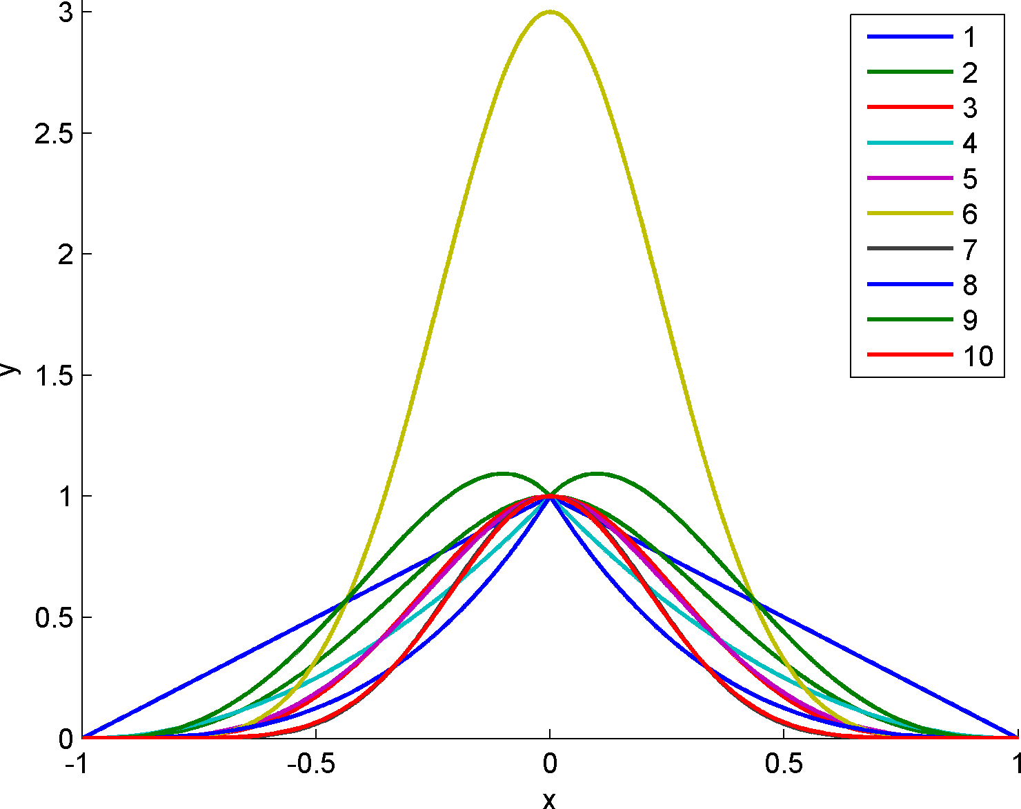

2.1 Radial basis function interpolation

RBF interpolation was originally introduced by [44] and is based on computing of the distance of two points in any $k$ -dimensional space. It is defined by the function

$f(\bm{x})=\sum\limits_{j=1}^{M}{\lambda_{j}\varphi(\left\|\bm{x}-\bm{x}_{j}% \right\|)}$ (5)

where $\lambda_{j}$ are weights of the RBFs, $M$ is the number of the radial basis functions, i.e. the number of interpolation points, and $\varphi$ is the radial basis function. For a given dataset of points with associated values, i.e. in the case of scalar values $\{\bm{x}_{i},h_{i}\}_{1}^{M}$ , the following linear system of equations is obtained:

$\displaystyle h_{i}=f(\bm{x}_{i})=\sum\limits_{j=1}^{M}{\lambda_{j}\varphi(% \left\|\bm{x}_{i}-\bm{x}_{j}\right\|)}$ $\displaystyle\quad\text{for }\forall i\in\{1,\ldots,M\}$ (6)

where $\lambda_{j}$ are weights to be computed; see Fig. 2 for a visual interpretation of Eqs (5) or (2.1) for a $2\frac{1}{2}D$ function. Point in $2\frac{1}{2}D$ is a $2D$ point associated with a scalar value. The same also applies to $3D$ point associated with a scalar value, thus $3\frac{1}{2}D$ point.

Figure 2.

Data values, the RBF collocation functions, the resulting interpolant.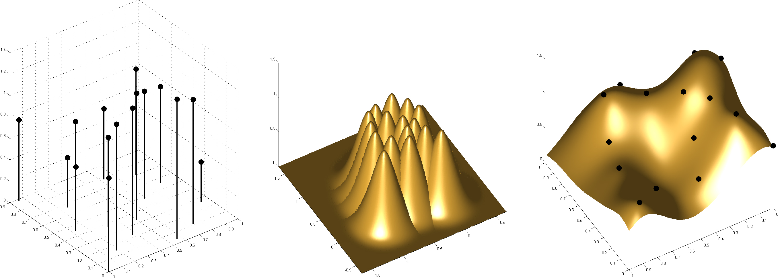

Equation (2.1) can be rewritten in a matrix form as

$\bm{A\lambda}=\bm{h}.$ (7)

As $\varphi(\|\bm{x}_{i}-\bm{x}_{j}\|)=\varphi(\|\bm{x}_{j}-\bm{x}_{i}\|)$ the matrix $\bm{A}$ is symmetrical.

The RBF interpolation can use “global” or “local” functions. When using “global” radial basis functions, the matrix $\bm{A}$ will be full, but when using “local” radial basis functions, the matrix $\bm{A}$ might be sparse, which can be beneficial when solving the system of linear equations $\bm{A\lambda}=\bm{h}$ .

In the case of the vector data, i.e. $\{\bm{x}_{i},\bm{h}_{i}\}_{1}^{M}$ values $\bm{h}_{i}$ are actually vectors, the RBF is to be performed for each coordinate of the vector $\bm{h}_{i}$ .

3. Proposed approach

In this section we describe our new proposed approach for large data sets RBF interpolation. The proposed interpolation uses space subdivision to speed-up the computation and to significantly reduce high memory requirements [37, 15]. The algorithm consists of three main steps. The first one is the space subdivision, the second one is the RBF interpolation and the last one is the joining procedure of interpolated cells (“blending”) to create the final interpolation. The pseudo-code of the proposed approach is in Algorithms 3.1 and 3.1. We show the speed-up of the proposed algorithm compared to the standard one for RBF interpolation as well.

3.1 Space subdivision

The approach Pseudocode of the proposed RBF interpolation method.[1] RBF $Points∼{}P$ $P_{i}=\{\textbf{x}_{i},h_{i}\}$ cells in grid Enlarge cell by $1/\epsilon$ where $\epsilon$ is the shape parameter $p\leftarrow$ Points in enlarged cell Compute RBF interpolation of $p$ Pseudocode of interpolated value calculation using the proposed RBF interpolation method.[1] RBF $Point∼{}p$ $p=\{x,y\}$ Find neighboring cells Compute distances to cells Compute interpolated RBF values for all cells Blend RBF values together using distances to cells proposed is based on a divide and co- nquer (D&C) strategy, and therefore input data set is split into several subsets. In our case, we will use a rectangular grid of the size $n\times m$ domains for $2\frac{1}{2}D$ input data, resp. $n\times m\times l$ domains for $3\frac{1}{2}D$ input data. The grid does not have to be necessarily regular and we can adjust it according to the properties of the input data set. We will use an orthogonal regular grid of domains for simplicity of explanation of the proposed approach.

The input points need to be divided into some cells according to the created grid for the space subdivision. Every domain of the grid needs to be enlarged to a cell and contains a few more points from the neighborhood, see Fig. 3. We will present the reason for this later in this paper.

The input points need to be divided into some number of cells. This number can be estimated according to the memory available. The RBF interpolation matrix for $n$ points in the cell has the size $n\times n$ elements, which are usually stored as double precision numbers. The size of the matrix in bytes is given as

$\textit{size}=\textit{sizeof}∼{}(\textit{double})\cdot n^{2}=8n^{2}∼{}(\textit% {Byte}).$ (8)

Using this formula we can easily find out the maximal average number of points in cells, see Fig. 4, and set up easily the size of the grid needed for the subdivision.

Data points are generally scattered, so it might be further possible in the extreme case that nearly all points lie within one cell. In this case it would be necessary to split this cell again. Another possible case is when no point lie inside a cell. In this case, the shape parameter and grid size for RBF interpolation is inappropriately selected and must be changed in the sense that the influencing of the basis function is greater and sufficient for the data interpolation [41].

Figure 3.

$2D$ regular orthogonal grid with one cell visualized. Each cell contains points from the grid domain plus points from the overlapping parts with neighborhood domains.

3.2 Cells RBF interpolation

Now, we have all input points divided into overlapping cells and thus can do the RBF interpolation. Radial basis functions have one parameter, which is the shape parameter $\epsilon$ . In the proposed approach, we use the “local” radial basis functions (CSRBFs), as they have the restricted maximal distance for the influence of the RBF interpolation. The shape parameter should be chosen so, that $\frac{1}{\epsilon}$ is equal to the size $r$ of the overlapping of each domain (Fig. 3), resp. vice versa. Points on the border of a cell are exactly $r$ away from the grid domain and RBF center points with a larger distance than $r$ will not have any influence on the interpolated value inside a domain of the grid.

Points inside a cell need to be interpolated using the RBF interpolation with CSRBF. This interpolation is done using the standard calculation of the linear system of Eq. (2.1). Each cell is interpolated as an independent cell and thus the calculation can be done totally in parallel. This parallel calculation will increase the performance and speed-up the RBF computation for each cell. The only problem that can arise is the memory consumption, as we need to store multiple interpolation matrices at once, so this should be kept in mind when computing the size of a grid for space subdivision.

For each cell we get one set of weighting values of the RBF interpolation $\bm{\lambda}=[\lambda_{1},\lambda_{2},\ldots,\lambda_{n}]^{T}$ . These values have to be stored for later use. The matrix used for their calculation, i.e. the RBF interpolation matrix, can be discarded.

Figure 4.

The size of the RBF interpolation matrix for different number of interpolated points. The matrix is stored in double precision and its size is in MB if full matrix structure is used. The memory requirements are 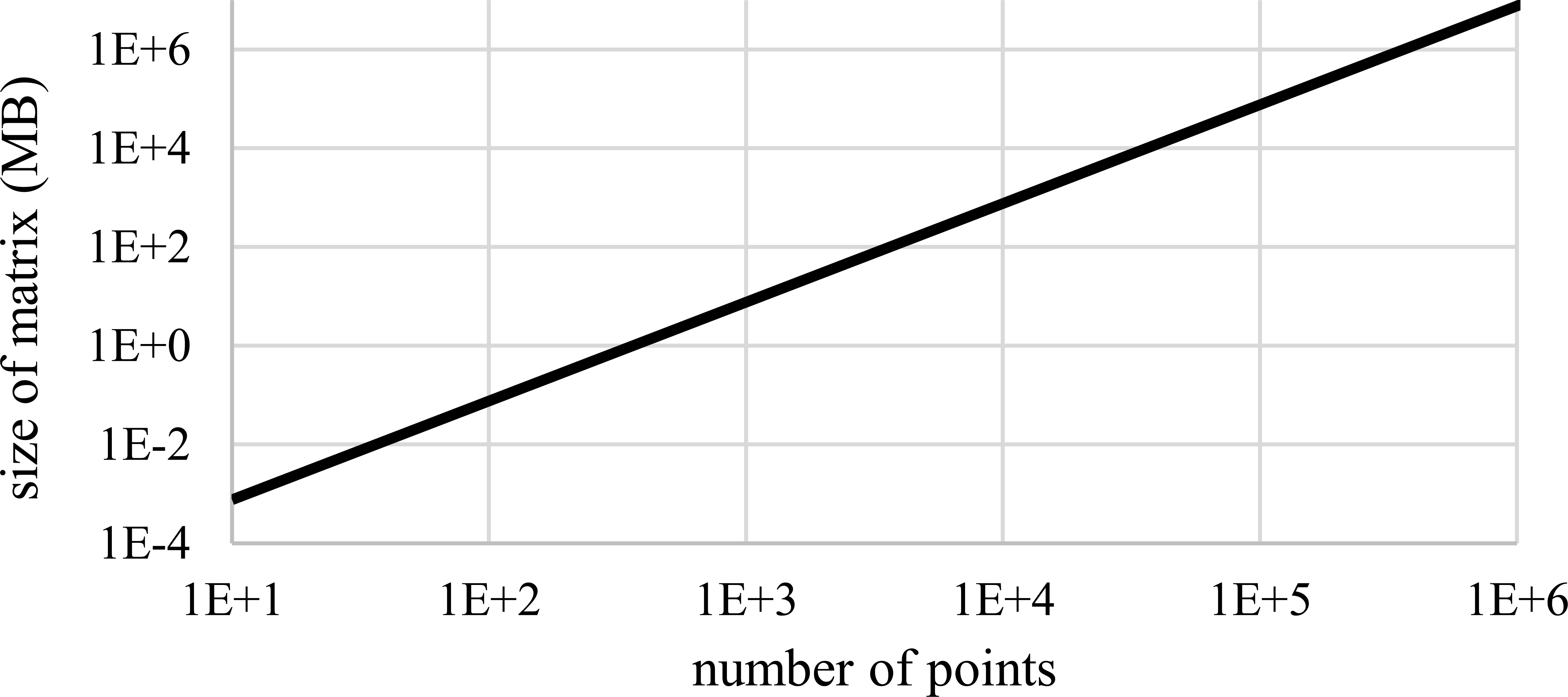$O(N^{2})$ , where $N$ is the number of points.

3.3 Blending of cells and reconstruction function

The interpolated cells computed in the previous step are overlapping each other. In this section, we show how to join, i.e. blend, them together to create a final continuous interpolation function that covers all the cells and thus all the input points for the interpolation as well.

The total width of overlapping parts is $2r$ . To blend all the neighborhood cells together, we will do some kind of bilinear interpolation (“blending”) between them. The computed value from each cell needs to be multiplied with a coefficient $\alpha$ . The coefficients $\alpha_{i}$ are computed as

$\alpha^{\prime}=\min\left(1,∼{}\frac{\textit{distance}∼{}\textit{from}∼{}% \textit{the}∼{}\textit{border}}{2r}\right),$ (9)

where distance from the border is the shortest distance from the location to the border and it is calculated using the Euclidean metric. However, for the axes-aligned grid, the distance can be calculated using Chebychev metric, which is defined as

$\textit{distance}(P,Q)=\max_{i}(|p_{i}-q_{i}|),$ (10)

where $P=[p_{1},\ldots,p_{k}]^{T}$ and $Q=[q_{1},\ldots,q_{k}]^{T}$ are two points in $k$ -dimensional space.

Figure 5.

Bilinear interpolation between cells for the overlapped areas. Red part of color represents the coefficient for the main cell value, green part of color represents the coefficient for the down cell value and blue part of color represents the coefficient for the right cell value. The value for the corner cell is calculated as 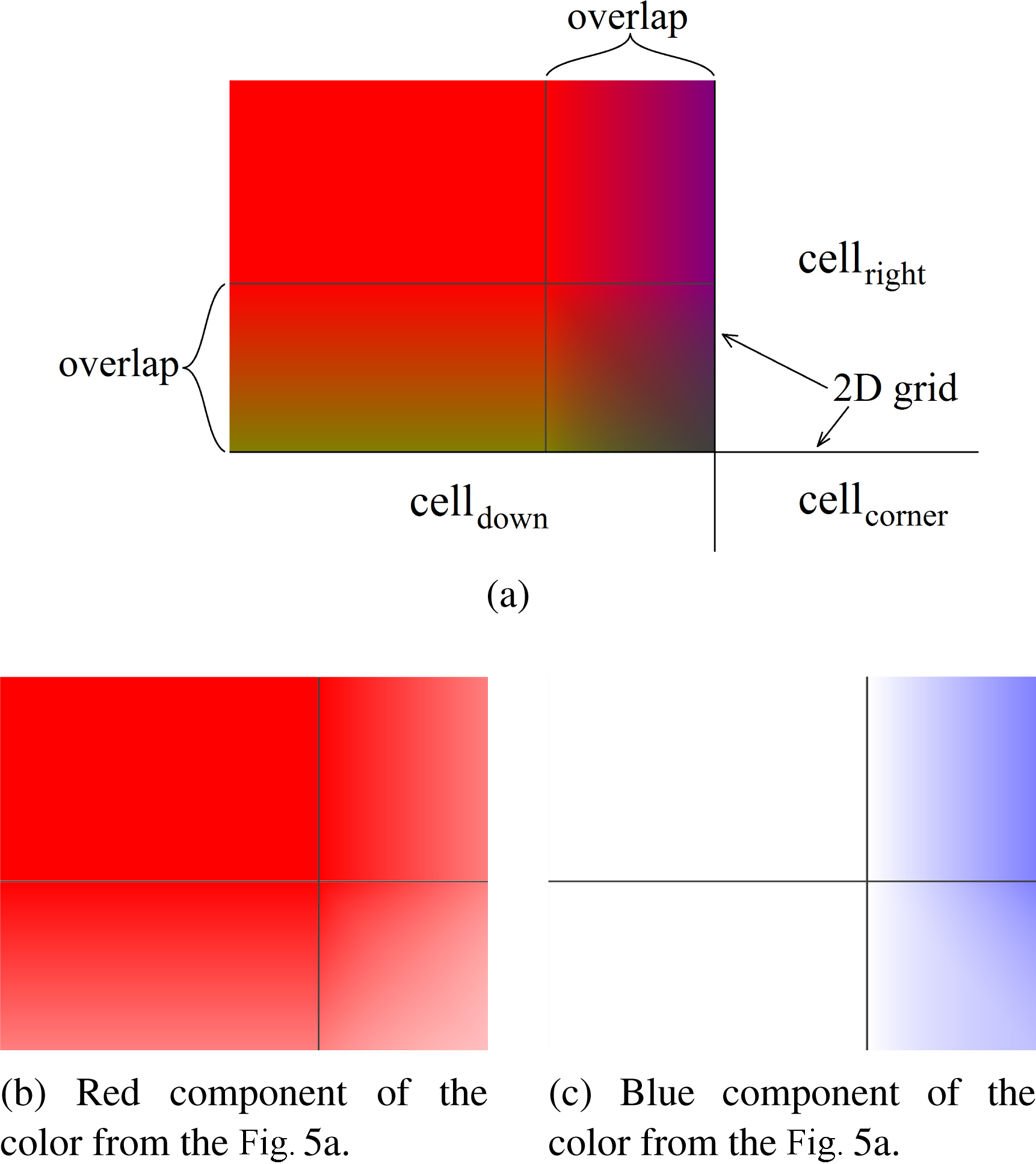$1-(\textit{red}∼{}+∼{}\textit{green}$ $+∼{}\textit{blue})$ .

The final coefficients $\alpha_{i}$ are computed using Eq. (9) as

$\alpha_{i}=\frac{\alpha{{}_{i}}{{}^{\prime}}}{\sum\limits_{j=1}^{2^{k}}\alpha{% {}_{j}}{{}^{\prime}}},$ (11)

where $k$ is the dimension, i.e. $k=2$ for $2\frac{1}{2}D$ or $k=3$ for $3\frac{1}{2}D$ input data. The visual representation of coefficients is shown in Fig. 5.

Knowing all the coefficients $\alpha_{i}$ and all function values from the RBF interpolations of cells, we can compute the final value of the proposed radial basis function interpolation algorithm for large scattered data interpolation .

$f(\bm{x})=\sum\limits_{i=1}^{2^{k}}{\alpha_{i}\left({\sum\limits_{j=1}^{M_{i}}% {\lambda_{j}\varphi\left(\left\|\bm{x}-\bm{x}_{j}^{(i)}\right\|\right)}}\right% )},$ (12)

where $k$ is the dimension, i.e. $k=2$ or $k=3$ , $M_{i}$ is the number of points in the $i$ -th cell, $\alpha_{i}$ is the coefficient from Eq. (11) and $\bm{x}_{j}^{(i)}$ are interpolation points in a cell.

During the blending phase we perform the interpolation between the interpolations of cells. The result of the blending phase is thus again the interpolation of all input points, as the resulting function passes through all input points.

Figure 6.

Visualization of a grid.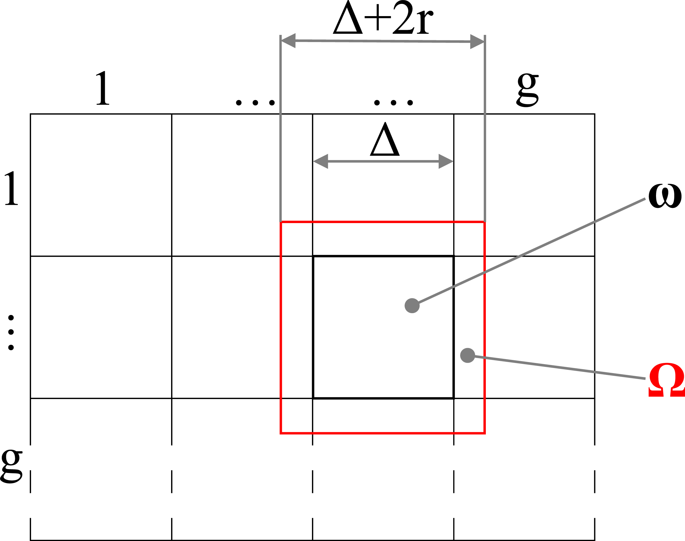

3.4 Speed-up of the proposed approach (interpolation)

The proposed approach uses space subdivision to speed-up the calculation of radial basis function interpolation and to reduce the needed memory as well. In the following, we will use the notation shown in Fig. 6.

The value $g$ is equal to the number of divisions in each dimension, $k$ is the dimension, $\Delta$ is the size of one domain, $r$ is the size of the overlap for each cell and is equal to the radius of the RBF.

The number of points $n$ in the area $\omega$ can be estimated in the case of uniform distribution as

$n=\frac{N}{g^{k}},$ (13)

where $N$ is the total number of points for the interpolation and $g$ is equal to the number of divisions in each dimension. Every domain $\omega$ is enlarged by the overlap $r$ , see Fig. 3, at every side of the domain; thus the enlargement of the domain is equal to

$\xi=\frac{\Delta+2r}{\Delta}=1+\frac{2r}{\Delta}.$ (14)

The average number of points in the enlarged cell $\Omega$ is equal to

$m=\frac{N}{g^{k}}{\xi}^{k}.$ (15)

When computing the RBF interpolation, we need to solve a system of linear equations (LSE). Let us assume that solving an LSE of size $N\times N$ has the time complexity $O(N^{3})$ . The time complexity of our proposed interpolation for one enlarged cell $\omega$ , i.e. the cell $\Omega$ , is

$O\left(\left(\frac{N}{g^{k}}\xi^{k}\right)^{3}\right).$ (16)

Therefore, the expected speed-up of the proposed algorithm compared to the standard one is

$\displaystyle\nu=\frac{O\left(N^{3}\right)}{O\left(g^{k}\left(\frac{N}{g^{k}}% \xi^{k}\right)^{3}\right)}=O\left(\frac{N^{3}}{g^{k}\left(\frac{N}{g^{k}}\xi^{% k}\right)^{3}}\right)$ $\displaystyle=O\left({\left(\frac{g^{2}}{\xi^{3}}\right)}^{k}\right),$ (17)

where $\nu\gg 1$ for the most grid resolutions, as can be seen in Fig. 7, which was generated for $\Delta=1$ and the overlap $r=0.2$ , i.e. $20\\$ overlap at each side of every domain. It should be noted, that the axis for $\nu$ is in logarithmic scaling.

Figure 7.

Expected speed-up of the proposed algorithm according to Eq. (3.4) for different numbers 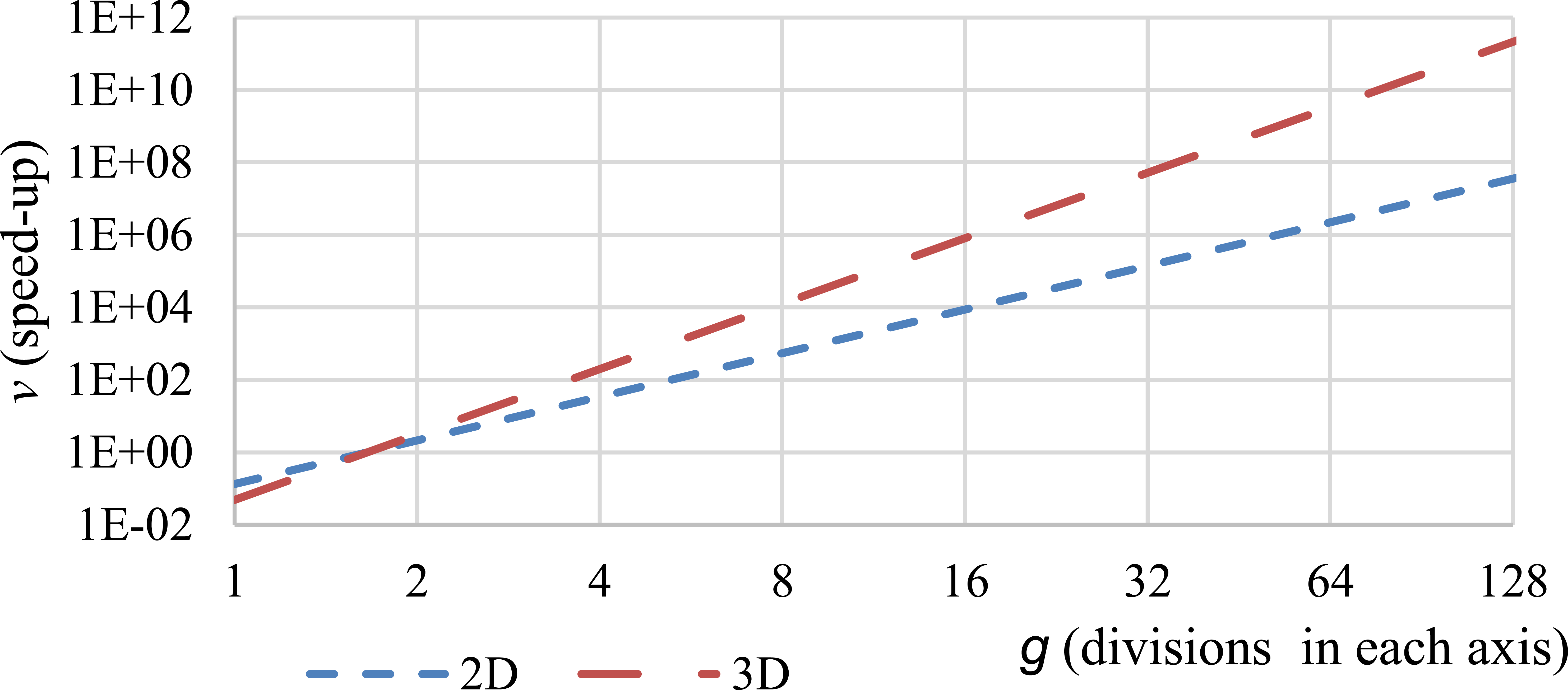$g$ , i.e. resolution of the grid, for $\Delta=1$ and the overlap $r=0.2$ .

The time complexity of our proposed approach for the RBF interpolation is

$O\left(g^{k}\left(\frac{N}{g^{k}}\xi^{k}\right)^{3}\right)=O\left(\frac{N}{n}% \left(n\xi^{k}\right)^{3}\right),$ (18)

where $n$ and $\xi$ can be constants. Then the only variable in Eq. (18) is $N$ . Thus, the time complexity of the proposed approach is $O(N)$ , but only in cases when the data points are uniformly distributed. Otherwise the worst time complexity of the proposed approach is $O(N^{3})$ .

3.5 Speed-up of the proposed approach (function evaluation)

The proposed approach does not speed-up only the RBF interpolation calculation, but it also speed-up the evaluation of the interpolation function as well. The time complexity of the function evaluation for the standard RBF is

$O(N).$ (19)

The time complexity of the function evaluation for our proposed approach for the RBF interpolation is

$O\left(2^{k}\frac{N}{g^{k}}\xi^{k}\right).$ (20)

Using Eqs (19) and (20), we can compute the speed-up of our proposed algorithm when computing one function value of the RBF interpolation:

$\displaystyle\eta=\frac{O\left(N\right)}{O\left(2^{k}\frac{N}{g^{k}}\xi^{k}% \right)}=O\left(\frac{N}{2^{k}\frac{N}{g^{k}}\xi^{k}}\right)$ $\displaystyle=O\left(\left(\frac{g}{2\xi}\right)^{k}\right).$ (21)

For most grid resolutions the speed-up $\eta\gg 1$ , as can be seen in Fig. 8, which was generated for $\Delta=1$ and the overlap $r=0.2$ , i.e. $20\\$ overlap at each side of every domain. It should be noted that the axis for $\eta$ is in logarithmic scaling.

Figure 8.

Expected speed-up of function evaluation using the proposed algorithm according to Eq. (3.5) for different numbers 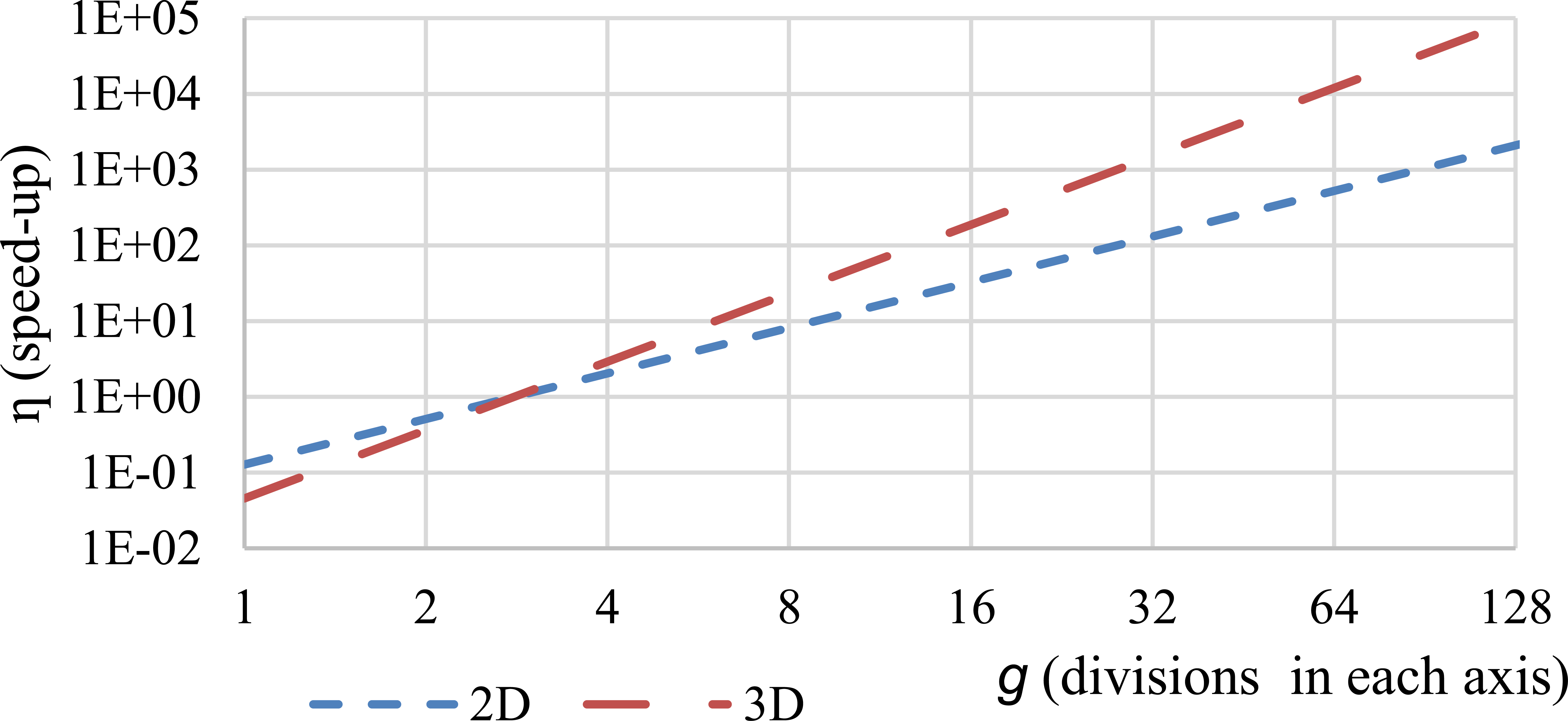$g$ , i.e. resolution of the grid, for $\Delta=1$ and the overlap $r=0.2$ .

4. Results

In this section we show the results of our proposed approach. This approach for RBF interpolation is especially convenient for large data set interpolation. However, in the first sub-section we test it for the case of its simplicity only with small synthetically generated data sets to show some basic results of the proposed method for RBF interpolation.

In the second sub-section we tested our approach with real data sets. The second example is a data set containing more than $6\times 10^{6}$ points, which is much more than the standard RBF interpolation is able to handle and compute on an ordinary computer.

Any of the CSRBFs in Eq. (2) can be used for the proposed RBF interpolation. However, in the tests we present results for one basis function, namely

$\varphi_{5}(r)=(1-\epsilon r)^{4}_{+}(4\epsilon r+1).$ (22)

We tested the proposed approach also with global radial basis functions, specifically with thin plate spline (TPS) and Gauss function. The results for global RBFs are very similar to those when using CSRBFs.

The implementation of the RBF interpolation was performed in MATLAB and tested on a PC with the following configuration:

•

CPU: Intel ${}^{\@setsize{\scriptsize}{8pt}{\viipt}{\@viipt}\textregistered}$ Core™ i7-920 (4 $\times$ 2.67 GHz $+$ hyper-threading),

•

memory: 22 GB RAM,

•

operation system: Microsoft Windows 8 64 bit.

Figure 9.

$10^{4}$ input points were used to test the proposed RBF interpolation.

4.1

2\frac{1}{2}D

synthetic data

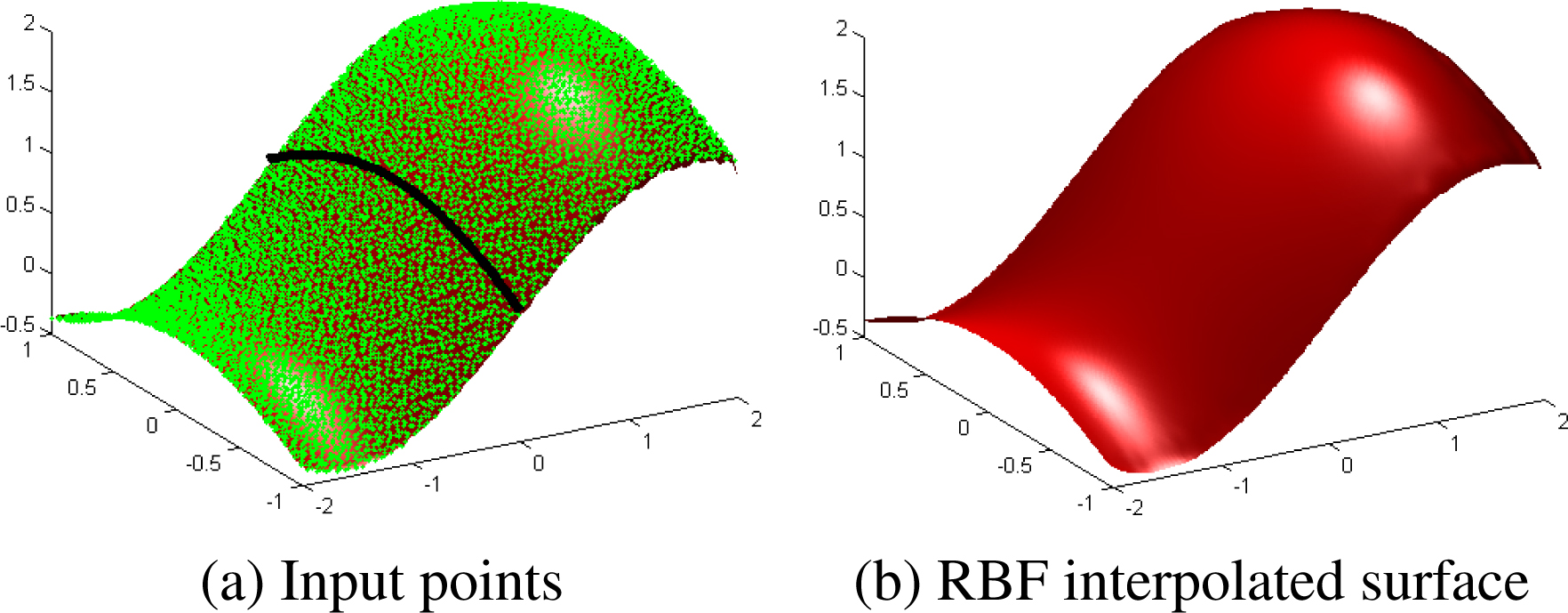
We first tested the proposed RBF interpolation on a synthetic data set of points using the function

$f(x,y)=\sin(x)+\cos(y).$ (23)

We sampled the function at $10^{4}$ random positions with a Halton distribution (A.1 in [26]) where $x\in\left[-2;2\right]$ and $y\in\left[-1;1\right]$ , see Fig. 9a. We used a grid of the size $2\times 1$ and $\epsilon=5$ and $10\\$ of overlapping. The result of the proposed interpolation can be seen in Fig. 9b. The result is continuous.

We measured the difference of function values of the two RBF interpolations of two cells on their common border before the blending phase, see Fig. 9a. We should note that for this test, we did not blend these two RBF interpolations. The absolute difference between those two cells along the border is visualized in Fig. 10.

We measured the difference of function values between each cell RBF interpolation and the original function Eq. (23) on the common border before the blending phase. The difference between each cell and the original function is visualized in Fig. 11. We should note that for this test, we did not blend these two interpolations in any way.

Figure 10.

Absolute difference in function values along the common border between the RBF interpolations of two cells without the blending phase, i.e. without the linear interpolation between cells.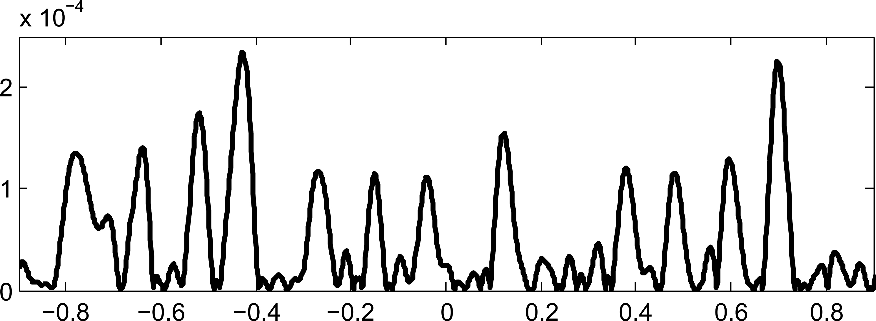

Figure 11.

Difference of function values along the common border between the interpolation of each cell without the blending phase, i.e. without the linear interpolation between cells, and the original function Eq. (23).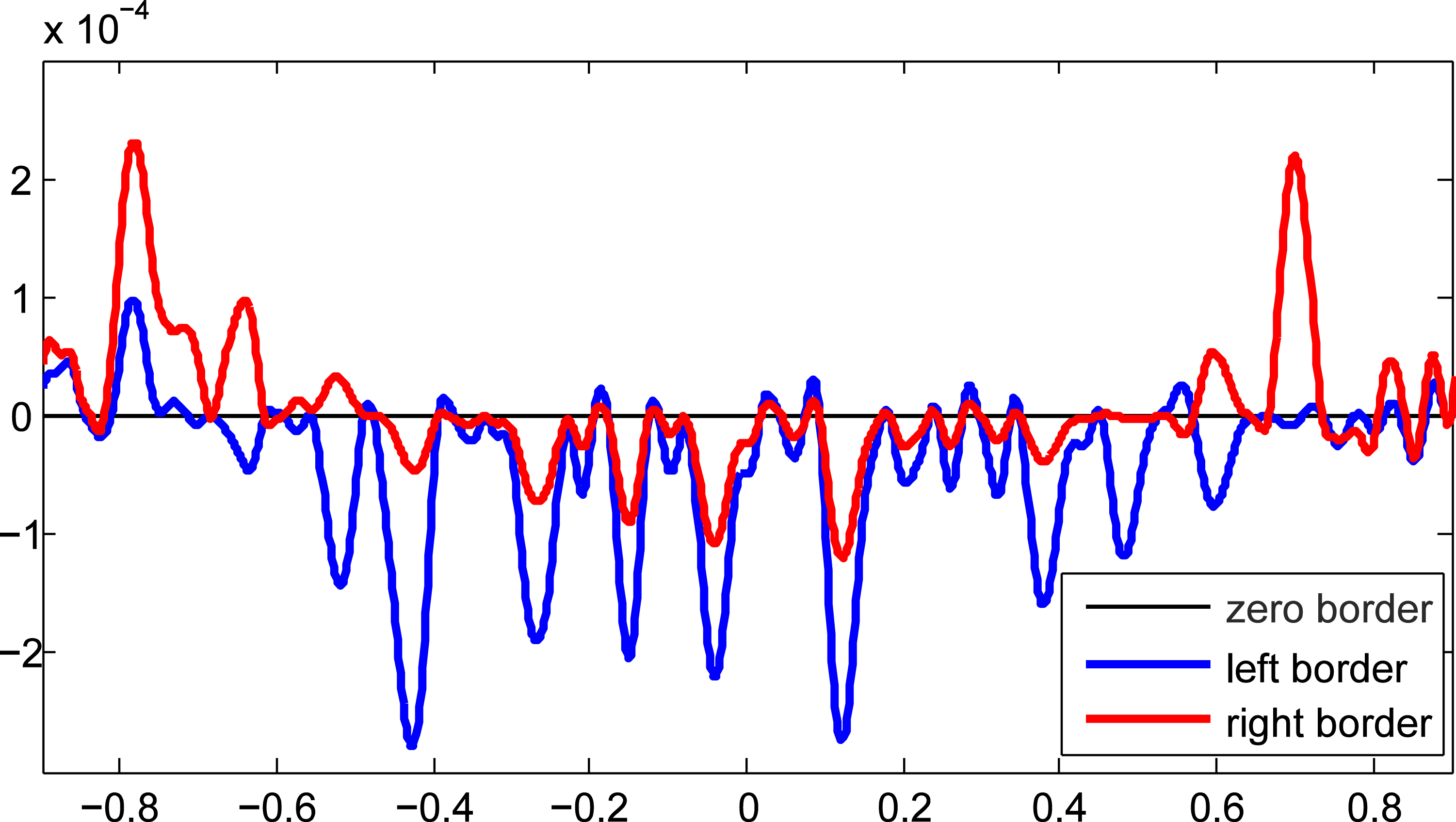

Figure 12.

Difference in function values between the proposed RBF interpolation and the original function Eq. (23).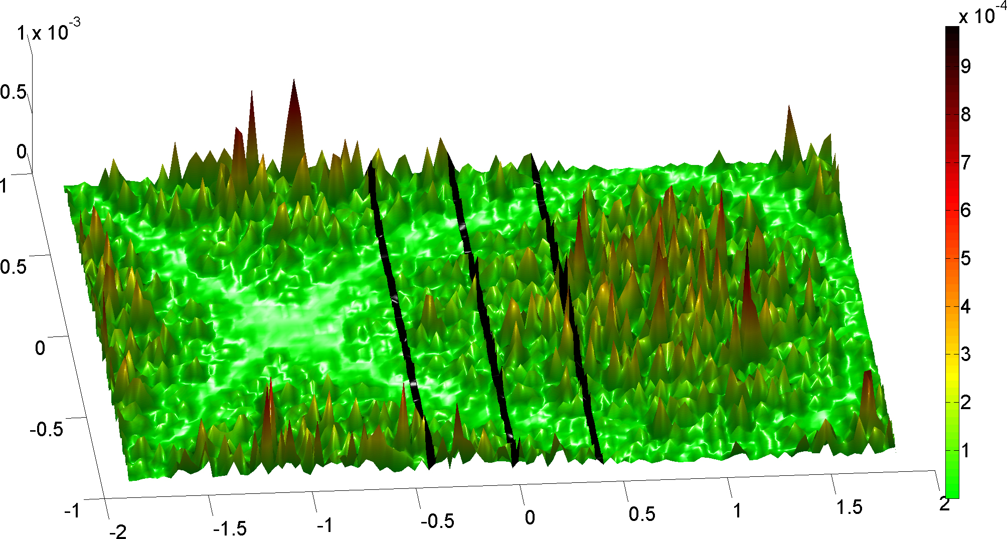

Two cells are interpolated using RBF interpolation independently and then blend together. We measured the interpolation error between blended cells and the original function Eq. (23). The results are visualized in Fig. 12. The proposed interpolation is continuous, without any disparity between domains.

We measured the interpolation error between the proposed RBF interpolation and the original function Eq. (23) on the common border. The error is visualized in Fig. 13. It can be seen that the error has a behavior similar to that represented in Fig. 12.

Figure 13.

Difference in function value between the proposed RBF interpolation with blending phase and the original function Eq. (23).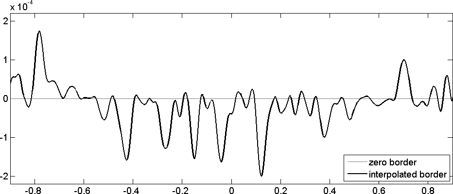

Figure 14.

Absolute difference in function values along the common border between interpolations of the two cells for different sizes of overlapping parts (for $100\\$ $\textit{error}=0$ ).

The same measurement as in Fig. 10 was done for a different percentage of cells overlapping, see Fig. 14. It can be seen that the error decreases and for $100\\$ overlapping this error is $0$ , as both the RBF interpolations use all points for the interpolation of their cell. It means that the proposed RBF interpolation is continuous, i.e. waterproof.

However, we need also to measure the quality of this RBF interpolation. For this purpose we compare our proposed method using the space subdivision with the standard RBF interpolation method (2.2 in [26]) using $2\times 10^{4}$ randomly sampled points with the uniform distribution of the function [26]:

$\displaystyle f(x,y)=3(1-x)^{2}e^{(-x^{2}-(y+1)^{2})}$ $\displaystyle-10\left(\frac{x}{5}-x^{3}-y^{5}\right)e^{(-x^{2}-y^{2})}$ $\displaystyle-\frac{1}{3}e^{(-(x+1)^{2}-y^{2})},$ (24)

where $x\in\left[-3;3\right]$ and $y\in\left[-3;3\right]$ .

We used a grid of size $4∼{}\times∼{}4$ and the shape parameter with the size $20\\$ of the domain edge length. The result of this interpolation is presented in Fig. 15. The standard RBF interpolation used the same points, the same basis function and the same shape parameter for interpolation.

To evaluate the quality of the interpolation we generated $1.5\times 10^{5}$ randomly sampled points with Halton distribution where $x\in\left[-3;3\right]$ and $y\in\left[-3;3\right]$ . Then we computed function values of both the interpolations and evaluate the absolute error of each interpolation. For each point $P_{i}=\left[x_{i},y_{i}\right]^{T}$ we compute absoluteerror

$\textit{Err}_{i}=\left\|\textit{RBF}(P_{i})-f(x_{i},y_{i})\right\|_{2},$ (25)

where $\textit{RBF}(P_{i})$ is the interpolated value at point $P_{i}$ using standard RBF interpolation on the whole dataset and RBF interpolation of the proposed approach, $f(x_{i},y_{i})$ is the function value of Eq. (4.1). The Fig. 16 presents distribution histograms of the interpolation errors.

Table 1

Average interpolation error of the proposed approach and the standard RBF interpolation. The interpolation error difference between both measured methods is only 0.03%

	Proposed approach	Standard RBF
		interpolation
Mean absolute error	$3.1371\cdot 10^{-4}$	$3.1362\cdot 10^{-4}$

Figure 15.

The result of RBF interpolation using the proposed method with space subdivision.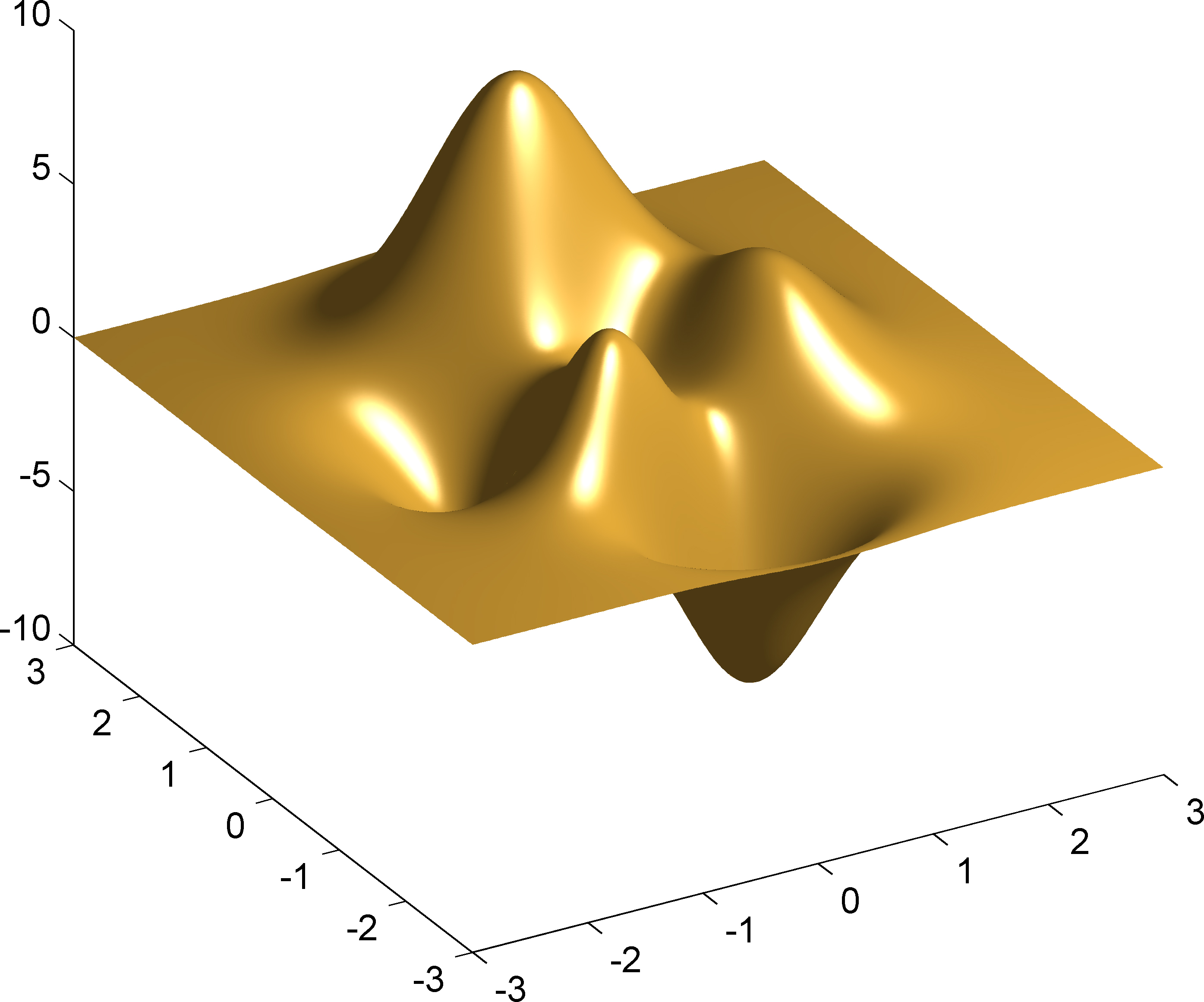

Figure 16.

Histograms of interpolation errors.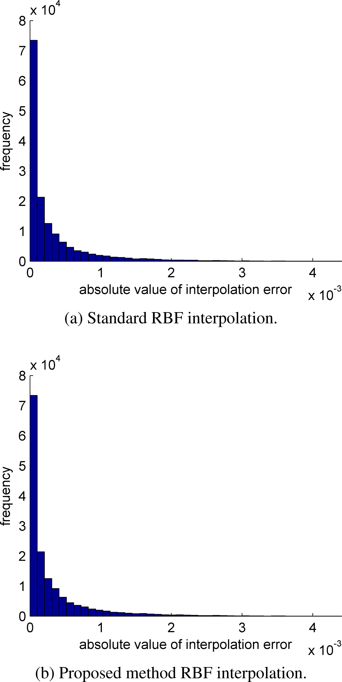

As both histograms in Fig. 16 are visually identical, we created a difference histogram between the two histograms. In Fig. 17 it can be seen that the interpolation errors distribution is almost identical. The difference in both histograms differs only slightly, see Fig. 17. Thus both interpolations have almost the same quality.

We also computed the average interpolation error for each RBF interpolation. The result is in Table 1. We can see that both average interpolation errors are almost the same, there is only a difference of $0.03\\$ . Knowing all results from quality measurements we can say that our proposed RBF interpolation has almost identical quality as the standard RBF interpolation.

Figure 17.

Difference of histograms in Fig. 16. Positive values mean that the standard RBF interpolation has more errors with the specific absolute value of interpolation error and the negative values mean the same for the proposed method for RBF interpolation.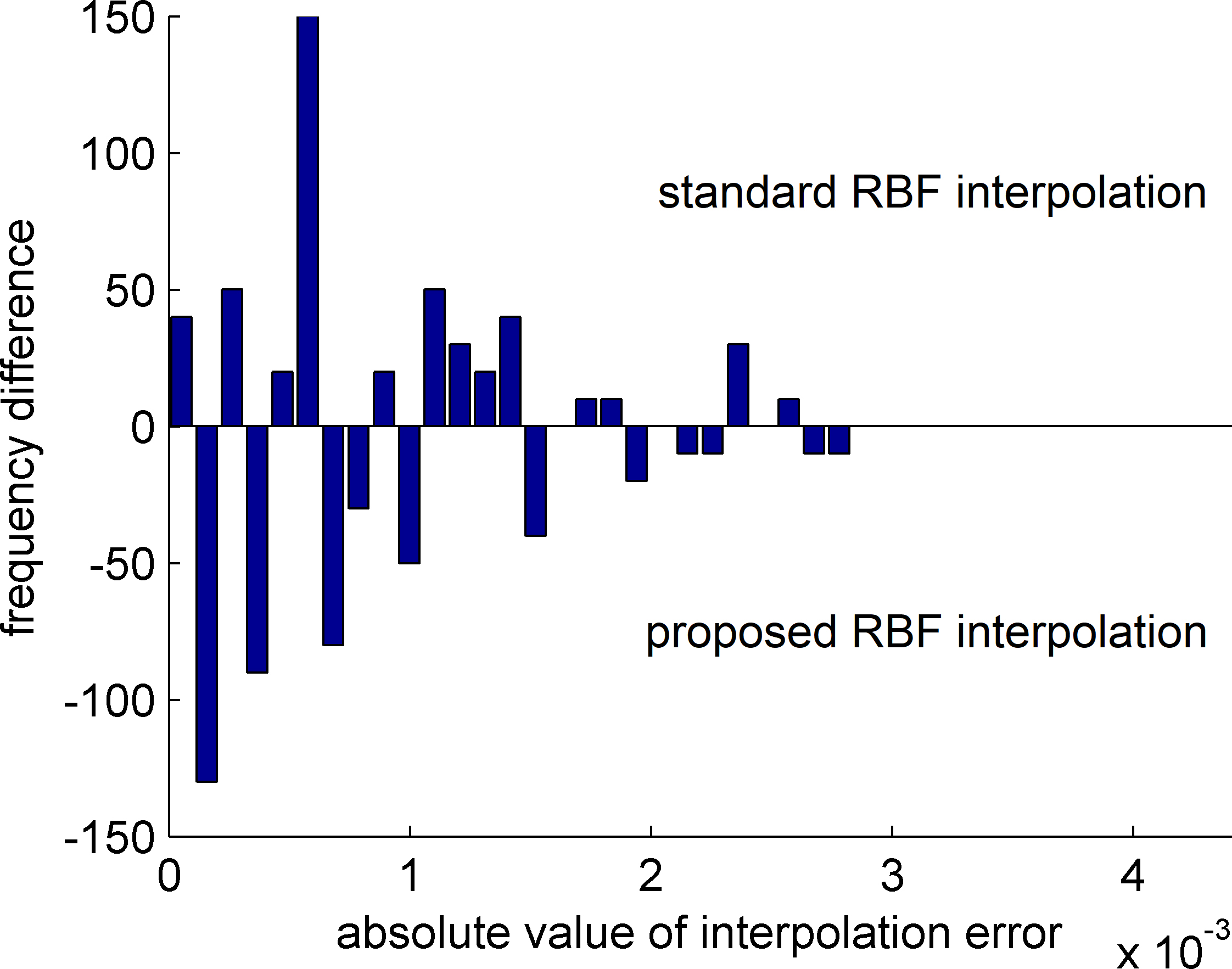

Figure 18.

Visualization of the interpolated terrain produced only as a visualization of each domain separately. The orthogonal grid used for the space subdivision with resolution of $29\times 46$ is visualized on the terrain as well.

4.2 Real data set

The proposed approach is mainly suited for large data interpolation. For this reason we chose to use a real data set. The LiDAR data of Mount Saint Helens1 in Skamania County, Washington, contains scanned height data. The data set consists of 6,743,176 $2D$ points with associated heights, i.e. $2\frac{1}{2}D$ data.

We chose to divide the input data set into a regular grid in a way such that the inside of a domain is going to be on average 5,000 points. To make square domains, we created a grid of the size $29\times 46$ , as the data range is around $2.1\cdot 10^{4}∼{}ft\times 3.3\cdot 10^{4}∼{}ft$ , i.e. $6.4\cdot 10^{3}∼{}m\times 1.0\cdot 10^{4}∼{}m$ , in $x$ and $y$ coordinates. The visualization of the created grid domains is in Fig. 18.

To perform the RBF interpolation, we needed to choose the shape parameter $\epsilon$ of the CSRBF. We tested different values of the shape parameter and selected the best shape parameter which has the size of $20\\$ of the domain edge length. Each cell will therefore contain approximately

$5{,}000\times(1+2\cdot 0.2)^{2}=9{,}800$ (26)

points. The number of points inside the cell is almost double times more than number of points inside the domain, but the final speed-up will still be very high. For clarity we can estimate the speed-up of the proposed algorithm compared to the standard one as:

$\textit{speed}\textnormal{-}up=\frac{6{,}743{,}176^{3}}{29\times 46\times 9{,}% 800^{3}}\approx 2.4\times 10^{5}.$ (27)

It can be seen that the speed-up is significant and we save a lot of calculations. The expected speed-up of the function evaluation is

$\textit{speed}\textnormal{-}up=\frac{6{,}743{,}176}{2^{2}\times 9{,}800}% \approx 172.$ (28)

This means that each RBF function computation for a given $\bm{x}$ is approximately $172$ times faster.

Moreover, the standard algorithm for RBF interpolation would require around 330 TB to save the full interpolation matrix to the memory when double precision is used.

The data set divided into cells was interpolated one cell after another. We used one RBF interpolated cell to reconstruct the terrain inside one domain of the grid without blending step. The result can be seen together with the grid of domains in Fig. 18.

Table 2

Parallel speed-up of the proposed method compared to the serial version of this method

Number of threads	1	2	4
Speed-up	1	1.791	3.172

Figure 19.

Visualization of the final result of the proposed method for large scattered data interpolation with the RBF and space subdivision.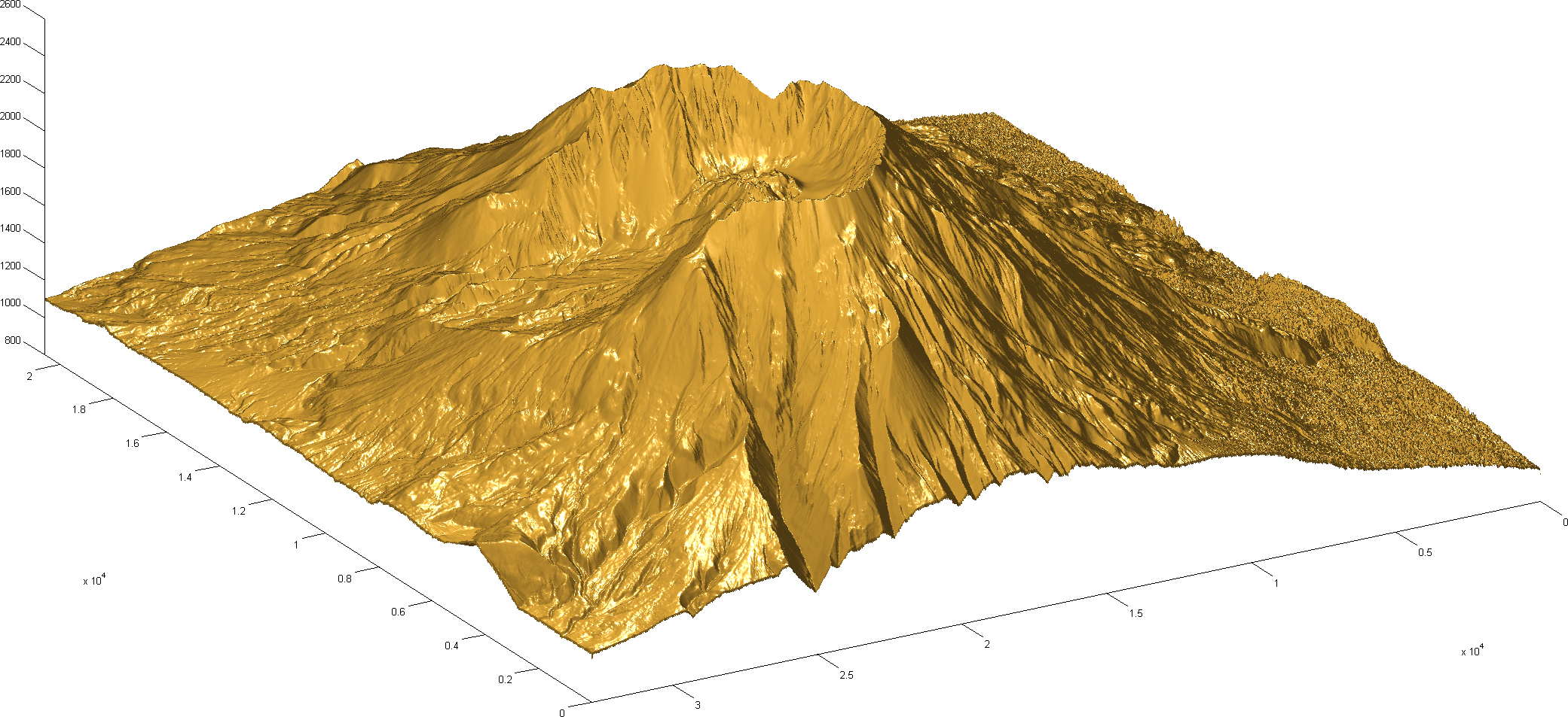

Figure 19 presents the result of the proposed RBF interpolation method. We used Eq. (12) to compute interpolation of the height values of the terrain for the visualization. This terrain does not have any discontinuity because of the proposed blending procedure.

The proposed algorithm can be easily parallelized as the RBF interpolation of each cell of the grid can be done separately and thus in parallel. We measured the running time of the interpolation when using $1$ or $2$ or $4$ threads. The resulting speed-up in MATLAB is in the Table 2. It can be seen that the speed-up is high because the threads do not have to wait for any synchronization and are independent of each other.

Figure 20.

Visualization of the interpolated terrain produced only as a visualization of each domain separately. The orthogonal grid used for the space subdivision with resolution of 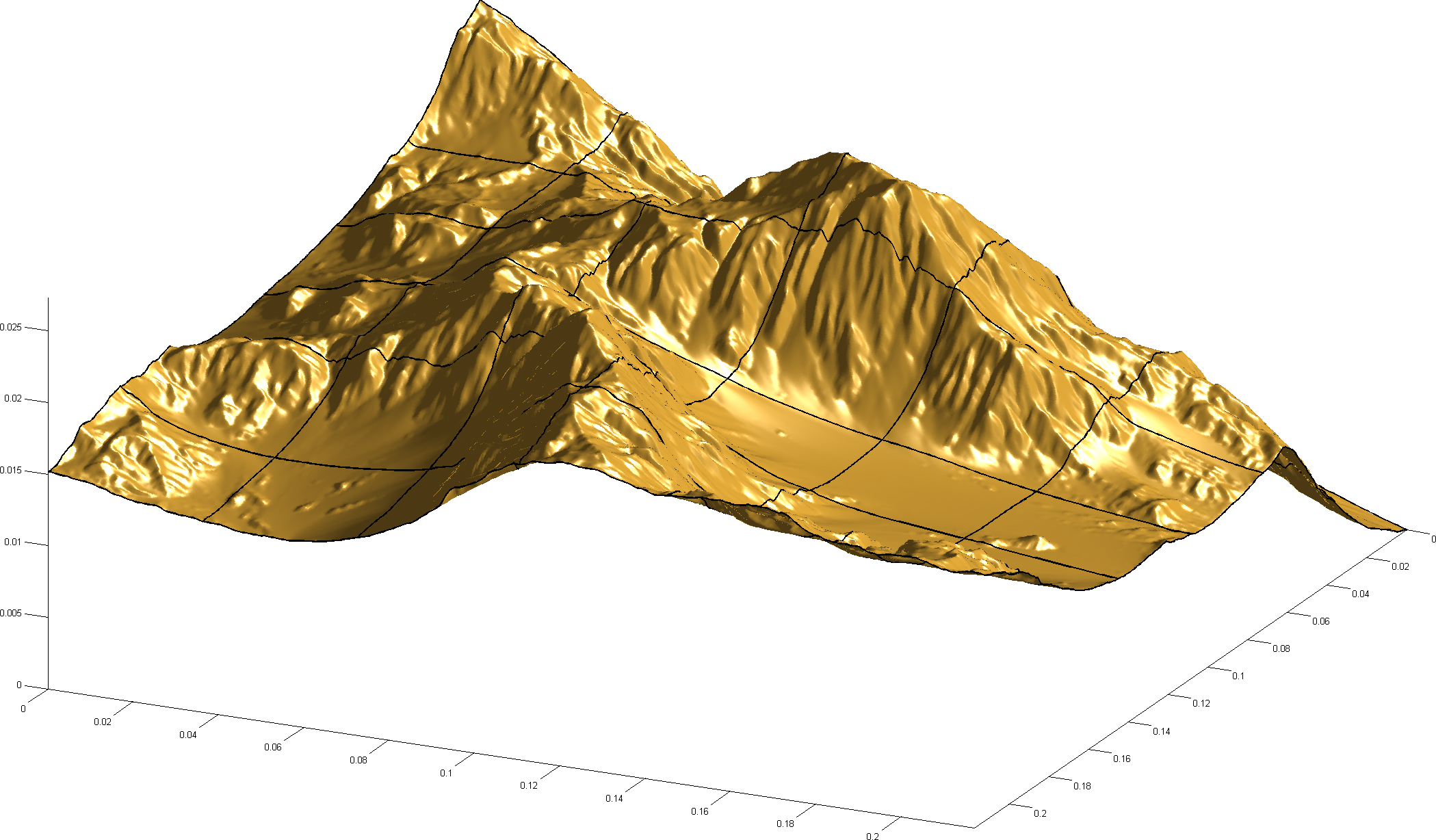$6\times 6$ is visualized on the terrain as well.

We tested our proposed approach with another data set too. We chose a model of the terrain2 which contains 131,044 points with associated heights, i.e. $2\frac{1}{2}D$ data.

We divided the input data set to a regular grid so that a domain contains 3,000 points in average. We created a grid of the size $6\times 6$ , with the data range is around 0.2172 miles $\times$ 0.2172 miles in $x$ and $y$ coordinates. The visualization of the created grid of domains is in Fig. 20.

For the shape parameter, we used the size of $20\\$ of the domain edge length. Therefore, each cell contains around

$3{,}000\times(1+2\cdot 0.2)^{2}=5{,}880$ (29)

points. It is almost double times more, but the final speed-up will still be very high. We can estimate the speed-up of the proposed algorithm compared to the standard one:

$\textit{speed}\textnormal{-}up=\frac{131{,}044^{3}}{6\times 6\times 5{,}880^{3% }}\approx 3\times 10^{2}.$ (30)

It can be seen that the speed-up is significant and will save us a lot of calculations. The speed-up of interpolating function evaluation is

$\textit{speed}\textnormal{-}up=\frac{131{,}044}{2^{2}\times 5{,}880}\approx 5.6.$ (31)

Moreover, the standard algorithm for the RBF interpolation needs around 128 GB to save the full interpolation matrix to the memory when double precision is used.

The data set divided into cells was interpolated one cell after another. We did a visualization of this RBF interpolation without doing any blending procedure. We used one RBF interpolated cell to reconstruct the terrain inside each domain of the grid. The result can be seen in Fig. 20, together with a visualization of the grid.

Figure 21 presents the result of the proposed RBF interpolation method. We used Eq. (12) to compute the height values of the terrain for the visualization. This terrain is continuous and does not have any discontinuity because of the proposed blending procedure.

Figure 21.

Visualization of the final result of the proposed method for large scattered data interpolation with the RBF and space subdivision.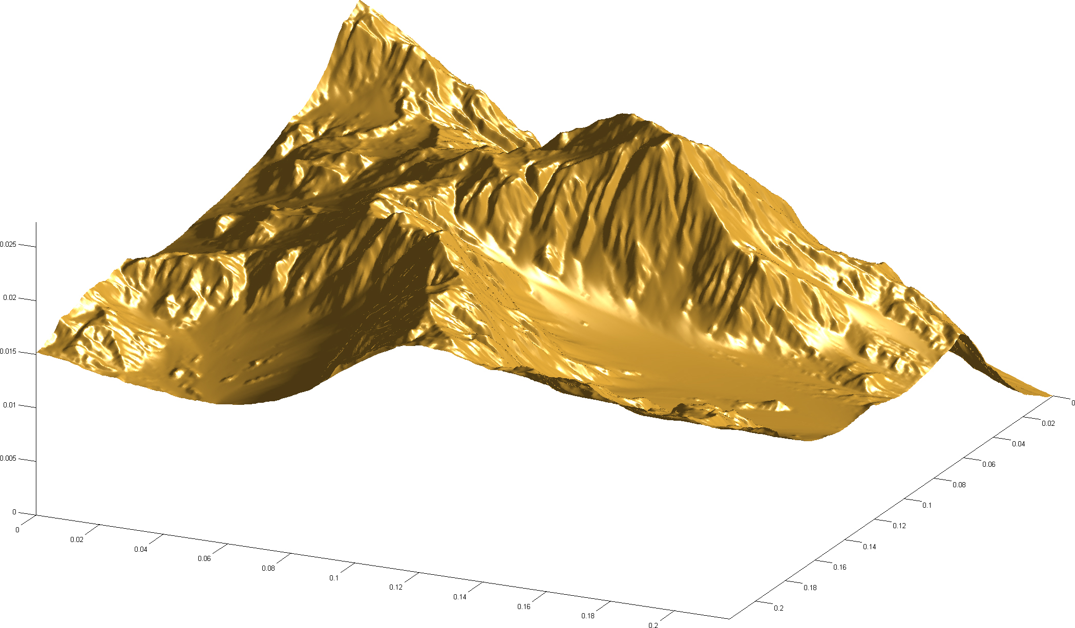

If CSRBF is used, many elements in the interpolation matrix are equal to zero, as the matrix is sparse in general. To decrease the memory requirements and be able to solve large interpolation matrices we can use a sparse matrix data structure. There are several existing sparse matrix representations. e.g. [45, 46, 37]. The main difference among existing storage formats is the sparsity pattern, or the structure of nonzero elements, for they are best suited. In our implementation, the coordinate format is used, which is briefly described in the following.

The coordinate (COO) format [47] is the simplest storage scheme. The sparse matrix is represented by three arrays: $d a t a$ , where the nonzero values are stored, $r o w$ , where the row index of each nonzero element is kept, and $c o l$ , where the column indices of the nonzero values are stored. The benefit of this format is its generality, i.e. an arbitrary sparse matrix can be represented by the COO format and the required storage is always proportional to the number of nonzero values. The disadvantage of the COO format is that both row and column indices are stored explicitly, which reduces the efficiency of memory transactions (e.g. read operations).

Moreover, note that the elements in the interpolation matrix are zero for far away points, when CSRBFs are used. Therefore, we do not need to compute the elements for all pairs of points, so the kd-tree (A.2 in [26]) is used for computing the interpolation matrix.

As the proposed approach also needs to be compared with the standard one for RBF interpolation; we used the dataset in Fig. 21 which contains 131,044 points for interpolation. For the shape parameter for RBF interpolation we used the size of $1/30$ of the data range. We measured the running times of our algorithm running in sequential version for different grid resolutions and computed the speed-up compared to the standard algorithm for RBF interpolation, see Table 3. Both methods are using sparse matrix with COO format and kd-tree structure. We also measured the memory requirements and the results are in Table 4.

Table 3

Speed-up of the proposed approach for large scattered data interpoloation compared to the standard RBF interpolation. Both methods are using sparse matrix with COO format and kd-tree structure

Grid resolution	4 $\times$ 4	6 $\times$ 6	8 $\times$ 8	10 $\times$ 10	12 $\times$ 12
Speed-up	1.69	1.83	2.06	2.28	2.57

According to the results in Table 3, the proposed algorithm is faster than the standard one and the speed-up is increasing with increasing of the grid resolution; both methods used the COO sparse matrix structure. We could not compute the speed-up when using the full matrix data structure as we were unable to fit such large data into the available memory for the standard algorithm.

Table 4

Memory requirements for our proposed method and for the standard RBF interpolation method. The proposed method was tested with full matrix data structure and also using sparse matrix with COO format together with kd-tree structure. The standard algorithm for RBF interpolation uses sparse matrix with COO format together with kd-tree structure

	Proposed method		Standard method
Grid size	kd-tree and	Full matrix	kd-tree and
	sparse matrix		sparse matrix
4 $\times$ 4	590 MB	6,900 MB
6 $\times$ 6	290 MB	2,300 MB
8 $\times$ 8	180 MB	1,000 MB	8,800 MB
10 $\times$ 10	125 MB	500 MB
12 $\times$ 12	95 MB	400 MB

According to the results in Table 4, the proposed approach has much lower memory requirements than the standard one. Therefore our approach enables to compute the RBF interpolation for very large datasets even on computers with standard memory size.

5. Conclusion

We presented a new approach for radial basis function interpolation of scattered data. It computes the interpolation on partly overlapping cells and then blends these interpolations together to create the final interpolation of the whole data set. This approach is especially efficient for large scattered data interpolation, as it reduces the memory required. It significantly speeds up computation of the interpolated value. The proposed approach is suitable for parallelization and it was tested on synthetic and large real data sets. It proved its robustness and high performance.

In future the proposed approach will be used for vector fields interpolation of large data sets based on [48, 49] and considering also vector field characteristics. We plan to modify the proposed method for $3D$ scattered data interpolation and approximation. In the case of $3D$ , point data will be split into overlapping cubes according to the grid. The joining phase, i.e. blending, will be almost the same as when blending $2D$ cells.

Footnotes

http://www.liblas.org/samples/.

http://www.badking.com.au/site/shop/environment/mountain-terrain/.

Acknowledgments

The authors would like to thank their colleagues at the University of West Bohemia, Plzen, for their discussions and suggestions, especially to Zuzana Majdisova, and anonymous reviewers for their valuable comments and hints provided. The research was supported by projects Czech Science Foundation (GACR) No. 17-05534S and SGS 2016-013.

References

Davis

. Interpolation and approximation. Courier Corporation 1975.

O’Rourke

Mallinckrodt

, et al. Computational geometry in C. Computers in Physics 1995; 9(1): 55-55.

Yang

Wang

Zhu

Peng

. Implicit surface reconstruction with radial basis functions. International Conference on Computer Vision and Computer Graphics, Springer 2007; 5-12.

Ohtake

Belyaev

Alexa

Turk

Seidel

. Multi-level partition of unity implicits. ACM Siggraph 2005 Courses, ACM 2005; 463-470.

Ohtake

Belyaev

Seidel

. A multi-scale approach to 3D scattered data interpolation with compactly supported basis function. 2003 International Conference on Shape Modeling and Applications (SMI 2003) 2003; 153-164, 292.

Yokota

Barba

Knepley

. PetRBF-A parallel O(N) algorithm for radial basis function interpolation with Gaussians. Computer Methods in Applied Mechanics and Engineering 2010; 199(25): 1793-1804.

Saad

Schultz

. GMRES: A generalized minimal residual algorithm for solving nonsymmetric linear systems. SIAM Journal on Scientific and Statistical Computing 1986; 7(3): 856-869.

Cai

Sarkis

. A restricted additive Schwarz preconditioner for general sparse linear systems. SIAM Journal on Scientific Computing 1999; 21(2): 792-797.

Cuomo

Galletti

Giunta

Starace

. Surface reconstruction from scattered point via RBF interpolation on GPU. Computer Science and Information Systems (FedCSIS), 2013 Federated Conference on IEEE 2013; 433-440.

10.

Süßmuth

Meyer

Greiner

. Surface reconstruction based on hierarchical floating radial basis functions. Computer Graphics Forum 2010; 29(6): 1854-1864.

11.

Haase

Martin

Offner

. Towards RBF Interpolation on Heterogeneous HPC Systems. Large-Scale Scientific Computing – 10th International Conference, LSSC 2015; 2015: 182-190.

12.

Beatson

Light

Billings

. Fast Solution of the Radial Basis Function Interpolation Equations: Domain Decomposition Methods. SIAM J Scientific Computing 2001; 22(5): 1717-1740.

13.

Farrell

Pestana

. Block preconditioners for linear systems arising from multiscale collocation with compactly supported RBFs. Numerical Lin Alg with Applic 2015; 22(4): 731-747.

14.

Ling

Kansa

. Preconditioning for radial basis functions with domain decomposition methods. Mathematical and Computer Modelling 2004; 40(13): 1413-1427.

15.

Majdisova

Skala

. A radial basis function approximation for large datasets. Proceedings of SIGRAD 2016; (127): 9-14.

16.

Smolik

Skala

Nedved

. A Comparative Study of LOWESS and RBF Approximations for Visualization. Computational Science and Its Applications – ICCSA 2016 – 16th International Conference, Part II 2016; 405-419.

17.

Mallet

. Discrete smooth interpolation. ACM Transactions on Graphics (TOG) 1989; 8(2): 121-144.

18.

Bui

Nguyen

Nguyen-Dang

. A moving Kriging interpolation-based meshless method for numerical simulation of Kirchhoff plate problems. International Journal for Numerical Methods in Engineering 2009; 77(10): 1371-1395.

19.

Royer

Wang

Zhang

. Factorial kriging for multiscale modelling. Journal of the Southern African Institute of Mining and Metallurgy 2014; 114(8): 651-659.

20.

Knopf

Sangole

. Interpolating scattered data using 2D self-organizing feature maps. Graphical Models 2004; 66(1): 50-69.

21.

Marinov

Kobbelt

. Optimization methods for scattered data approximation with subdivision surfaces. Graphical Models 2005; 67(5): 452-473.

22.

Katz

Rohlf

. Function-point cluster analysis. Systematic Biology 1973; 22(3): 295-301.

23.

Lounsbery

DeRose

Warren

. Multiresolution analysis for surfaces of arbitrary topological type. ACM Transactions on Graphics (TOG) 1997; 16(1): 34-73.

24.

Eck

DeRose

Duchamp

Hoppe

Lounsbery

Stuetzle

. Multiresolution analysis of arbitrary meshes. Proceedings of the 22nd Annual Conference on Computer Graphics and Interactive Techniques ACM 1995; 173-182.

25.

Pan

Skala

. A two-level approach to implicit surface modeling with compactly supported radial basis functions. Engineering with Computers 2011; 27(3): 299-307.

26.

Fasshauer

. Meshfree approximation methods with MATLAB. vol. 6. World Scientific; 2007.

27.

Skala

. Meshless interpolations for computer graphics, visualization and games. Eurographics 2015 – Tutorials 2015.

28.

Larsson

Fornberg

. A numerical study of some radial basis function based solution methods for elliptic PDEs. Computers & Mathematics with Applications 2003; 46(5): 891-902.

29.

Zhang

Song

Liu

. Meshless methods based on collocation with radial basis functions. Computational Mechanics 2000; 26(4): 333-343.

30.

Uhlir

Skala

. Reconstruction of damaged images using radial basis functions. Signal Processing Conference, 2005 13th European, IEEE 2005; 1-4.

31.

Karim

Adeli

. Radial basis function neural network for work zone capacity and queue estimation. Journal of Transportation Engineering 2003; 129(5): 494-503.

32.

Ghosh-Dastidar

Adeli

Dadmehr

. Principal component analysis-enhanced cosine radial basis function neural network for robust epilepsy and seizure detection. IEEE Transactions on Biomedical Engineering 2008; 55(2): 512-518.

33.

Yingwei

Sundararajan

Saratchandran

. Performance evaluation of a sequential minimal radial basis function (RBF) neural network learning algorithm. IEEE Transactions on Neural Networks 1998; 9(2): 308-318.

34.

Adeli

Karim

. Fuzzy-wavelet RBFNN model for freeway incident detection. Journal of Transportation Engineering 2000; 126(6): 464-471.

35.

Karim

Adeli

. Comparison of fuzzy-wavelet radial basis function neural network freeway incident detection model with California algorithm. Journal of Transportation Engineering 2002; 128(1): 21-30.

36.

Hsu

Lin

Yeh

. Supervisory adaptive dynamic RBF-based neural-fuzzy control system design for unknown nonlinear systems. Applied Soft Computing 2013; 13(4): 1620-1626.

37.

Majdisova

Skala

. Big geo data surface approximation using radial basis functions: A comparative study. Computers & Geosciences 2017; 109: 51-58.

38.

Prakash

Kulkarni

Sripati

. Using RBF Neural Networks and Kullback-Leibler distance to classify channel models in Free Space Optics. Optical Engineering (ICOE), 2012 International Conference on IEEE 2012; 1-6.

39.

Schagen

. Interpolation in two dimensions – a new technique. IMA Journal of Applied Mathematics 1979; 23(1): 53-59.

40.

Fornberg

Piret

. On choosing a radial basis function and a shape parameter when solving a convective PDE on a sphere. J Comput Physics 2008; 227(5): 2758-2780.

41.

Majdisova

Skala

. Radial basis function approximations: Comparison and applications. Applied Mathematical Modelling 2017; 51: 728-743.

42.

Skala

. RBF interpolation with CSRBF of large data sets. Procedia Computer Science 2017; 108: 2433-2437.

43.

Wendland

. Computational aspects of radial basis function approximation. Studies in Computational Mathematics 2006; 12: 231-256.

44.

Hardy

. Multiquadric equations of topography and other irregular surfaces. Journal of Geophysical Research 1971; 76(8): 1905-1915.

45.

Bell

Garland

. Implementing sparse matrix-vector multiplication on throughput-oriented processors. Proceedings of the Conference on High Performance Computing Networking, Storage and Analysis, ACM 2009; 18: 1-11.

46.

Simecek

. Sparse matrix computations using the quadtree storage format. Symbolic and Numeric Algorithms for Scientific Computing (SYNASC), 2009 11th International Symposium on IEEE 2009; 168-173.

47.

Gilbert

Moler

Schreiber

. Sparse matrices in MATLAB: Design and implementation. SIAM Journal on Matrix Analysis and Applications 1992; 13(1): 333-356.

48.

Smolik

Skala

. Vector Field Interpolation with Radial Basis Functions. Proceedings of SIGRAD 2016, Linköping University Electronic Press 2016; (127): 15-21.

49.

Smolik

Skala

. Classification of Critical Points Using a Second Order Derivative. Procedia Computer Science 2017; 108: 2373-2377.