A scalable approach based on deep learning for big data time series forecasting

Abstract

This paper presents a method based on deep learning to deal with big data times series forecasting. The deep feed forward neural network provided by the H2O big data analysis framework has been used along with the Apache Spark platform for distributed computing. Since H2O does not allow the conduction of multi-step regression, a general-purpose methodology that can be used for prediction horizons with arbitrary length is proposed here, being the prediction horizon, $h$ , the number of future values to be predicted. The solution consists in splitting the problem into $h$ forecasting subproblems, being $h$ the number of samples to be simultaneously predicted. Thus, the best prediction model for each subproblem can be obtained, making easier its parallelization and adaptation to the big data context. Moreover, a grid search is carried out to obtain the optimal hyperparameters of the deep learning-based approach. Results from a real-world dataset composed of electricity consumption in Spain, with a ten-minute frequency sampling rate, from 2007 to 2016 are reported. In particular, the accuracy and runtimes versus computing resources and size of the dataset are analyzed. Finally, the performance and the scalability of the proposed method is compared to other recently published techniques, showing to be a suitable method to process big data time series.

Keywords

Deep learning time series forecasting big data

1. Introduction

Increasing attention is being paid to the issue of time series forecasting nowadays [1], mainly due to its interdisciplinary nature. Almost all scientific disciplines consist of data sampled over time, which makes their forecasting a task of utmost significance and complexity. Participants in electricity markets (both demand and prices) are particularly interested in making accurate predictions [2], since their obtention is critical for many areas in order to increase benefits, such as planning, inventory management, or even in evaluating capacity needs.

When addressing big data problems, computational issues are usually encountered. Therefore, efficient algorithms must be developed to extract knowledge from massive data. These algorithms are developed using parallel and distributed computing techniques, which take advantage of the concurrency of multiple processors to execute processes at the same time [3, 4, 5]. Additionally, many artificial intelligence techniques have been inspired by the functioning of neural systems [6] and are currently reporting remarkable results in this research field [7, 8].

Deep learning is an emerging branch of machine learning that extends artificial neural networks [9]. One of the main drawbacks that classical artificial neural networks exhibit is that, with many layers, its training typically becomes too complex [10]. In this sense, deep learning consists of a set of learning algorithms to train artificial neural networks with a large number of hidden layers. Deep learning models are also sensitive to initialization and much attention must be paid at this stage [11].

For all the aforementioned, a preliminary deep learning-based approach to predict big data time series was published by the authors in [12]. By contrast, in this work, we now introduce a novel algorithm to forecast big data time series, based on deep learning architectures [13, 14]. In this new deep learning a new methodology to automatize the hyperparameters adjustment has been included. The sensitivity of the number of past values involved in the topology of the network is also analyzed. The accuracy of the proposed methodology is compared to other machine learning methods for big data time series applied to the same dataset. A thorough scalability analysis is also included, showing that the new approach is scalable, by varying the time series length and the number of executions threads, and more scalable than than most of the methods it has been compared to.

The algorithm has been developed for prediction horizons of arbitrary length, being suitable for the short, mid, and long-term forecasting. To achieve this goal, the proposed approach creates as many independent forecasting problems as samples are desired to be simultaneously forecasted. Later, each subproblem is individually addressed by computing different time slots within the historical data. Deep learning models have been embedded in the process and are responsible for making predictions. It is worth noting that the deep learning implementation used is that of the well-known H2O library [15], which is open source and has been conceived for distributed environments.

One of the most relevant features of this method lies in its inherent suitability to be launched in parallel environments, which turns this tool ready to be applied to big data. Moreover, Apache Spark has been used to load data in memory, significantly speeding up the whole process and thus decreasing the computation time.

The performance of the approach has been assessed in real-world datasets. Electricity consumption in Spain has been used as case study, and data from 2007 to 2016 in the usual 70%–30% training-test sets structure have been analyzed. Satisfactory results are reported in terms of both accuracy and processing time, outperforming those obtained by a linear regression, a decision tree and two ensemble techniques based on trees as Gradient-Boosted Trees, and Random Forest. A scalability analysis has also been conducted in order to show that the proposed method is fully suitable for big data.

In summary, the main contributions of this work are:

1)
We propose a new approach based on deep learning for electricity consumption forecasting. Due to the high computational cost of training a neural network, we develop the algorithm using an efficient distributed computing strategy, so that it can process very large time series.
2)
We develop a distributed grid search to determine the optimal parameters involved in the deep learning training. Such parameters have been found to be the number of layers and number of neurons, which eventually have a great impact on the performance of the algorithm.
3)
We conduct a wide experimentation using real electricity data, measured every 10 minutes for ten years, from the Spanish electricity market. We evaluate the prediction accuracy of the proposed algorithm and compare it with four state-of-the-art big data forecasting approaches, such as decision tree, gradient-boosted tree, random forest and linear regression [16]. The deep learning was the most accurate model achieving a MRE of 1.68%, which is a very promising result for the prediction of big electricity time series.
4)
We carry out a scalability study with the purpose of showing the suitability of the deep learning for processing large electricity time series. A detailed analysis of computing times for different time series lengths and number of threads is provided. Moreover, the scalability of the deep learning is also compared to the aforementioned state-of-the-art algorithms.

The remainder of the paper is structured as follows. Relevant related works are reviewed and discussed in Section 2. The proposed methodology is introduced in Section 3. Results are reported and discussed in Section 4. A comparative analysis to other well established forecasting strategies is shown in Section 5. Finally, the conclusions drawn are summarized in Section 6.
2. Related work

This section reviews relevant works in the context of big data, time series forecasting and deep learning. It also pays attention to works particularly devoted to forecast electricity demand.

Large datasets needs high performance hardware to be processed. Distributed computing can be used to leverage the existing hardware [17]. In this sense, Castillo et al. [18] introduced a novel approach, in which a SVM model was distributed. The authors emphasize that threads shared some data with each other during the training phase to enhance the learning process. Adeli and Hung described a concurrent gradient learning algorithm to train feed-forward neural networks applied to image recognition in [19]. In this research, the authors studied the behavior in terms of network speed by using large networks and vectorization. The use of graphics processing units (GPUs) has increased in recent years, due to the high performance – in terms of processing – they offer. Fang et al. [20] made a benchmark of a GPU memory system to quantify the capability of parallel accessing and broadcasting. The authors in [21] studied the performance of MPI parallel processing libraries on GPU clusters. In order to maximize the amount of data ingested by the training algorithm, the authors in [22] proposed a framework that uses parallel computing over GPU to train and combine a set of deep learning models. As another alternative, the authors in [23] have implemented the back-propagation learning algorithm on an FPGA board by performing several configurations and checking the runtime with other C and Matlab code implementations. This experimentation has shown that FPGA implementation is more efficient. To take advantage of the power of distributed computing, frameworks such as DistBelief [24], Minerva [25], ChainerMN [26] or TensorFlow [27], among others, are often used for deep learning problems. Erickson et al. summarized some of these distributed frameworks in [28].

The scalability of association rules techniques combined with evolutionary computation has also been addressed. The authors in [29] claimed to have developed a method particularly suitable to be applied to large datasets. Reported results are quite satisfactory and its use is encouraged for future works. More recently, a generic MapReduce framework to discover quantitative association rules in big data problems has also been proposed [30].

Recently, some studies have appeared discussing the performance associated with deep learning in the context of forecasting. In 2013, the temperature forecasting issue was analyzed in [31]. The authors paid particular attention to the hyperparameters of deep learning architectures and provided some clues on how to systematically adjust them.

Event driven stock market was also forecasted by means of a novel approach in 2015 [32]. Firstly, a deep convolutional neural network was used and, secondly, both short and long-term stock price fluctuations were modeled. Results were assessed on S&P 500 stock historical data, showing remarkable performance.

Dalto et al. [33] thoroughly reviewed the selection of variables in order to decrease computational time. As a result of their work, they were able to develop a deep learning based forecasting approach with better accuracy than that of compared standard artificial neural networks.

An interesting deep learning architecture, this time particularly designed for air quality prediction, was presented in [34]. Specially remarkable were the spa-tio-temporal correlations analyzed by means of a stacked autoencoder model for feature extraction that the authors used. The experimentation carried out and the comparisons made were useful to show how promising the approach is.

Later in 2016, another feature data based method was introduced in [35]. The application field was transportation forecast under data-driven perspective. Nam-ely, a deep learning model to forecast bus ridership at the stop and stop-to-stop levels was there adopted.

Deep learning methods have also been used in the field of health. A remarkable approach can be found in [36], in which the authors introduced a new deep learning approach based on voting schemes, with application to accurate early diagnose of Alzheimer cases. Morabito et al. presented a novel feature extraction method from time-frequency representation in EGG signals to differentiate the status of patients with Creutzfeldt-Jakob disease [37]. Acharya et al. also used CNN based deep learning applied to EEG signals to aide in the diagnosis of epilepsy in [38]. The authors in [39] explore a neural network based on adaptive differential evolution to determine the functional state of the human operator.

Another field of application for deep learning is civil infrastructure and construction. Some of these works are based on feature extraction to identify damage locations into buildings structures or pavements using convolutional neural networks [40, 41, 42]. In the same area, other deep learning architectures, such as Restricted Boltzmann Machine (RBM), have been also used [43, 44].

Image processing has proven to be one of the most fruitful fields of deep learning applications. Koziarski and Cyganek present in [45] a method for reducing the noise level in images using convolutional networks. The authors in [46] prove the effectiveness of applying a trained RBF polynomial network by fuzzy clustering and a trained forward propagation network with the backward propagation algorithm to extract the coastline position based on video images.

On the other hand, many authors combine the use of deep learning with metaheuristics. For instance, a deep learning metaheuristic model for time series forecasting using GPU was proposed in [47]. In the same way, Rafiei et al. proposed a novel machine learning model combining a genetic algorithm and a RBM in order to forecast the sale prices of houses [48].

Finally, some works related to electricity demand forecasting are also discussed in this section. In 2014, a hybrid method was presented with aim of forecasting time series [49]. In particular, the authors combined Hinton and Salakhutdinov’s networks with gradient descend and back propagation, as well as integrating some other preprocessing techniques.

Hu [50] proposed a novel neural network GM based model to forecast electricity consumption. Turkish Ministry of Energy and Natural Resources and the Asia Pacific Economic Cooperation energy database data were used with the purpose of evaluating the quality of the approach.

Marvuglia and Messineo [51] described a recurrent-neural-network-based model to forecast a time series with one hour as prediction horizon to evaluate the influence of the air-conditioning equipments.

Talavera-Llames et al. [52] proposed a forecasting algorithm, under the Apache Spark platform [53]. Data from the Spanish market were used to test the approach. Experimentation was conducted towards the successful application to big data time series. Preliminary reported results are of particular interest.

Also with data from the Spanish market, Pérez-Chacón et al. extracted demand profiles by means of scalable k-means algorithm [54]. The authors claimed the usefulness of using this information as input into a subsequent stage in the forecasting process. Big data time series were also used and profiles showed remarkable differences between working days and festivities and among seasons.

Large variations in consumption were analyzed in the work introduced in [55]. The authors deeply studied the influence that data size and temporal granularity may exhibit in such a context. The performance of the approach was assessed with data from Canada by means of different configurations of artificial neural networks and support vector regression, reporting promising results.

Mocanu et al. [56] proposed two new stochastic models based on artificial neural network to predict time series.

Conclusively, some surveys have been published collecting the latest works in which deep learning approaches have been developed, as seen in [57, 58, 59], where more than 100 studies are classified depending on a specific taxonomy such as the deep learning model used or the type of tasks that are dealt with. However, to the authors’ knowledge, none of them was developed to forecast very large time series. In summary, the study of the related work reveals that deep learning is already being used for big data, but mainly focused on applications related to image, video or audio. This is the first work that addresses deep learning for big data time series forecasting.

3. Methodology

The theoretical background in which this work is included is introduced in Section 3.1. Later, Section 3.2 introduces the proposed methodology itself.

3.1 Theoretical background

The research is included in the field of supervised learning, i.e. the instances composing the dataset are already labeled. Specifically, it is a regression task where a numeric value, called class, is intended to be forecasted. However, temporal order must be kept since data are sampled over time. To infer a model, from a part of the labeled data well-known as training set, is required to make a prediction. This model can be obtained by means of many techniques, such as linear regression, regression trees, nearest neighbors, neural networks or support vector machines. Deep learning is here proposed to forecast in a big data environment.

Many network architectures for deep learning are available depending on the characteristics of the target problem. Each architecture is designed to be applied to a particular problem, and therefore, each one works in a different way. Some of these architectures can be recurrent networks, convolutional networks, Hopfield networks, Kohonen networks or feed forward networks. A deep feed forward architecture is applied to forecast long time series in this work.

Feed forward neural networks are the most common network architectures for solving forecasting problems. The main characteristic of this type of network is that each neuron is a basic element of processing. This network is defined by the weights, which represent the interactions between each pair of neurons. Both weights and network topology are computed in the training phase.

Figure 1.

Multivariable forecasting problem.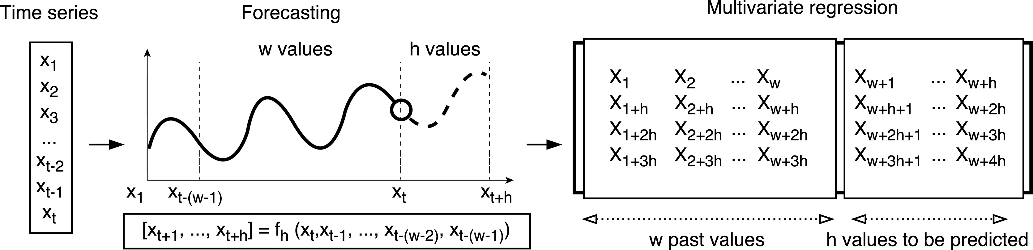

H2O is an open source platform to compute machine learning techniques into a single node or a cluster of machines in a distributed way, being scalable for big data projects. In particular, H2O is designed for distributed computing. It allows to build machine learning models on big data under a MapReduce processing paradigm. Thus, H2O automatically works in a distributed way by means of specific data structure called H2OFrame. Hence, once a dataset is loaded in a H2OFrame variable, the dataset is distributed in different chunks across all the nodes. Each partition of the H2OFrame is kept in memory, thus each node computes its part of the H2OFrame. Any operation over a H2OFrame is executed in parallel in each partition. Therefore, our approach is based on a modern distributed computation that consists in partitioning data and distributing them through different nodes in a cluster. H2O can also be integrated with Apache Spark to store data in memory instead of in hard disk. This framework includes a deep feed forward neuronal network, which has been used to forecast big data time series. The executions of this algorithm can be parameterized by a high number of parameters (known as hyperparameters) that will depend on the characteristics of the problem to be solved.

Figure 2.

Transformation from multivariate to univariate problem.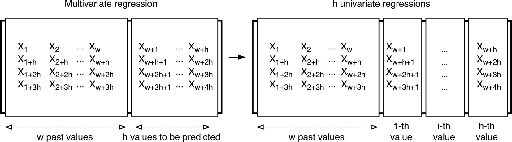

The most important parameters used in this study are described below:

•

Hidden. All possible numbers of hidden layers and numbers of neurons per layer are provided through this parameter.

•

L1. This parameter deals with the regularization to avoid overfitting, thus improving the generalization.

•

Epsilon and Rho. These parameters are related to the learning rate and they are used to avoid to achieve a local optima. Default values are 1E-8 and 0.99, respectively.

•

Activation. The activation function is used to model the type of relationship between inputs and outputs of the network. It has been set to the hyperbolic tangent.

•

Distribution. This parameter represents the loss function to be minimized.

•

Stop metric. It is the metric to be used for early stopping. The mean square error (MSE) was selected.

•

Stopping tolerance. This parameter stops the tra-ining of the deep network if an improvement of the established value is not achieved. Its default value is 1E-3.

•

Stopping round. If a moving average composed of the MSE of stopping_round models does not improve according to a given tolerance, then the deep learning algorithm stops. Its value by default is 5.

H2O allows the creation of a grid that generates all possible combinations according to the selected hyperparameters. Thus, it is possible to test several values of these parameters and generate a model for each combination. These models are sorted in ascending order according to the error, that is, from the best model to the worst model. A full description on how H2O works, in addition to all the parameters involved in the deep learning algorithm, can be found in [60].

3.2 Description of the methodology

This section describes the methodology proposed to forecast time series using the deep learning approach from H2O framework, under R programming language. The main goal of this study is to predict $h$ next values (hereinafter called prediction horizon) of a time series, expressed as $[x_{1},\ldots,x_{t}]$ , from $w$ previous values (hereinafter called historical data window). This process is also called multi-step regression, since more than one value has to be forecasted. A multi-step regression problem is illustrated in Fig. 1.

Figure 3.

Scheme of the proposed methodology.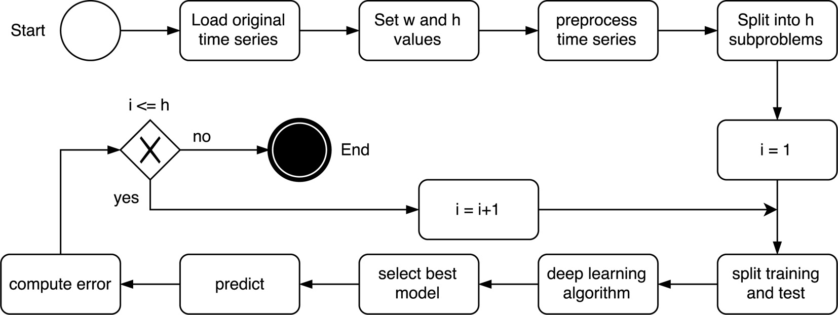

Formally, this problem can be formulated as it is presented in Eq. (3.2), where the goal is to find the model $f$ , after application of the deep learning method:

$\displaystyle[x_{t+1},x_{t+2},\ldots,x_{t+h}]=f(x_{t},x_{t-1},\ldots,x_{t-(w-1% )})$

Unfortunately, the deep learning algorithm included in the H20 framework does not support multi-step forecasting. Therefore, a new methodology has to be developed to achieve this goal. A possible way consists in splitting the main problem into $h$ forecasting subproblems, as shown in Fig. 2.

This new methodology can be formulated by using $h$ models, one for each forecasting subproblem, as shown in Eq. (2):

$\displaystyle x_{t+1}=f_{1}(x_{t},x_{t-1},\ldots,x_{t-(w-1)})$ (2) $\displaystyle x_{t+2}=f_{2}(x_{t},x_{t-1},\ldots,x_{t-(w-1)})$ (3) $\displaystyle x_{t+3}=f_{3}(x_{t},x_{t-1},\ldots,x_{t-(w-1)})$ (4) $\displaystyle\ldots$ (5) $\displaystyle x_{t+(h-1)}=f_{(h-1)}(x_{t},x_{t-1},\ldots,x_{t-(w-1)})$ (6) $\displaystyle x_{t+h}=f_{h}(x_{t},x_{t-1},\ldots,x_{t-(w-1)})$ (7)

On the one hand, the relations between consecutive values of the time series are missed in this methodology, as the future value is not predicted using the $w$ previous consecutive values. However, if the predictions of previous values were used to forecast, a greater error would be obtained, giving rise to a wrong prediction.

On the other hand, the obtention of $h$ independent models entails a higher computational cost than building just one model to predict all $h$ values. The deep learning method used in this work has an extra computational cost due to multiple models are computed, by combining different parameters in a grid search. However, since these models are independent, they can be easily parallelized.

A general scheme of the proposed methodology is illustrated in Fig. 3.

Figure 4.

Preprocessing of the original dataset.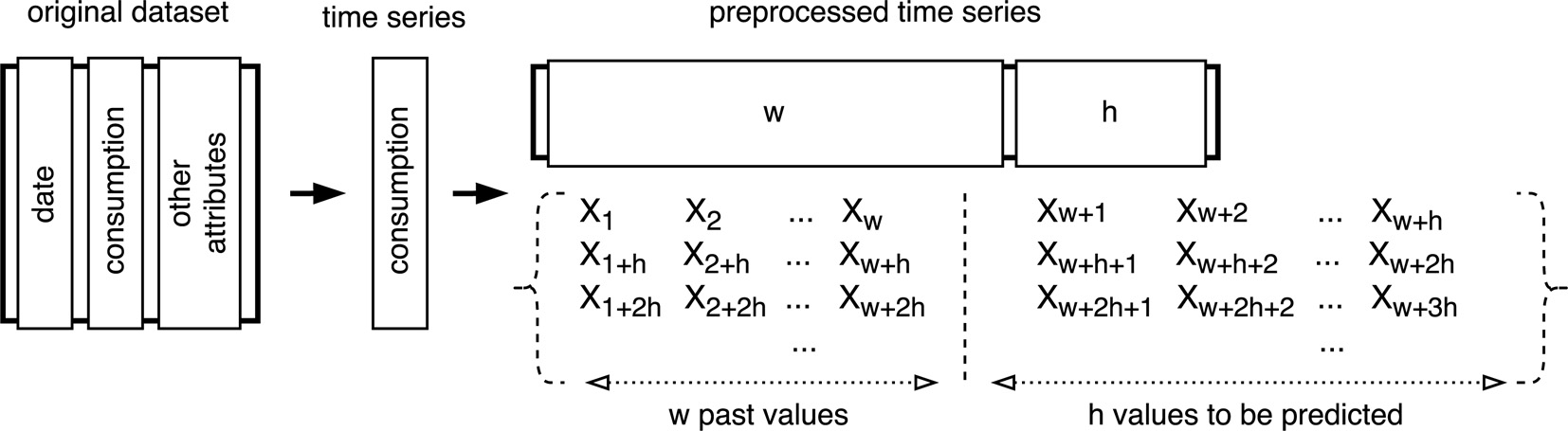

4. Results

This section presents the results obtained after applying the previously mentioned methodology to forecast the time series to be described in Section 4.1. Section 4.2 describes the experimental setup designed in order to obtain the optimal hyperparameters. After that, an analysis of the results is presented in Section 4.3. Finally, Section 4.4 shows the scalability of the proposed deep learning method, providing the computational time of the algorithm for time series of different length, and for different computing resources.

The hardware used in order to obtain the results reported here has been an Intel Core i7-5820K at 3.3 GHz with 15 MB of cache, 12 cores and 16 GB of RAM memory, working under an Ubuntu 16.04 operating system. The H2O framework was used to apply deep learning by using R language. This framework has available a feed-forward architecture and allows to configure a cluster to launch distributed executions.

4.1 Dataset description

The time series considered in this study is related to the electricity consumption in Spain from January 2007 to June 2016. It is a time series of 9 years and 6 months with a high sampling frequency (10 minutes), resulting in 497832 measures in total into a 33 MB file.

This time series needs to be preprocessed to build a dataset of $w+h$ attributes, being $w$ the number of past values used to forecast the $h$ next values as it is shown in Fig. 4. It can be noted that the number of instances of the final dataset can vary depending on $w$ and $h$ values. It is important to highlight that the $w+h$ value could not be multiple of the time series length. In that case, a row of the matrix has a number of columns lower than $w+h$ , being automatically removed.

The dataset was split into 70% for the training set and 30% for the test set, and in addition, a 30% from the training set has also been selected for the validation set in order to obtain the optimal parameters. The training set covers the period from January 1, 2007 at 00:00 to August 20, 2013 at 02:40. Therefore, the test set comprises the period from August 20, 2013 at 02:50 to June 21, 2016 at 23:40.

4.2 Design of experiments

The experimentation carried out is composed of two phases. First, the optimal parameters of the deep neural network will be calculated. Second, a scalability analysis will be performed using the optimal parameters found in the previous stage.

Table 1
MRE depending on the historical data window

w	Neurons per layer and subproblem	MRE
24	[20 50 90 100 30 100 70 100 90 20 70 50 60 100 80 70 60 70 70 100 80 100 60 90]	3.7648
48	[50 60 100 40 80 20 90 30 90 90 100 70 100 100 70 80 50 40 20 80 100 100 100 70]	2.8904
72	[30 50 70 80 100 100 60 40 40 60 40 60 90 70 40 80 50 20 50 20 80 60 70 80]	2.7259
96	[100 80 40 70 60 90 40 60 40 70 20 30 70 100 60 100 60 70 50 40 90 80 50 60]	2.5588
120	[30 30 90 70 20 70 70 80 30 80 80 70 60 70 60 80 80 40 40 30 70 90 100 100]	2.4180
144	[50 80 50 70 60 80 30 80 50 70 60 40 100 40 90 90 90 40 70 40 80 70 90 90]	1.8722
168	[30 80 90 60 60 100 40 80 30 80 50 100 40 80 90 40 70 70 70 60 90 70 100 100]	1.8439

The different settings applied to make the experiments are as follows:

The $w$ number of historical data has been set to 24, 48, 72, 96, 120, 144 and 168, corresponding to 4, 8, 12, 16, 20, 24 and 28 hours, respectively. After training and calculating the validation error for each value of $w$ , the value providing the smallest error is selected for the rest of experiments. A value of 168 was finally obtained.

The $h$ prediction horizon is set to 24, which represents a block of 4 hours to be predicted.

The number of hidden layers for applying the deep learning algorithm has been set from 1 to 5 layers and a number of neurons per layer varying from 10 to 100 by steps of 10.

The $l a m b d a$ regularization parameter is set to 0, 0.1, 0.01, 0.001 and 0.0001 values.

Gaussian and Poisson distribution functions have been tested.

Initial weights were provided by the UniformAdaptative distribution, which is an optimized initialization with regards to the size of the network. In the H2O architecture, it is possible to use normal or uniform distributions in addition to the UniformAdaptative. However, the UniformAdaptative distribution is considered the most adequate as 24 sub-problems with different network sizes are solved.

The remaining deep learning parameters are not specified, so they are set to default values described in the official H2O documentation [61].

Once the neural network has been trained, the optimal parameters are chosen to analyze the scalability of the proposed deep learning. Information related to the scalability study is detailed below:

The size of the time series is increased, multiplying its length by up to 2, 4, 8, 16, 32 and 64 times.

The number of local threads is set to 2, 4, 6, 8, 10 and 12 to verify how scalable is the deep learning method according to computing resources.

The deep learning method is executed on a cluster of 2 machines, using a total of 24 threads, to check its scalability on distributed computing resources.

The scalability of the deep learning is compared to other scalable methods recently published in the literature [16].

The Root Mean Squared Error (RMSE) and the mean absolute error (MAE) have been computed to evaluate the accuracy of the models in the training. On the other hand, the mean relative error (MRE) in percentage has been used to calculate the accuracy of the best deep learning model in the test set. The formulation of these errors is shown below:

$\displaystyle\textit{RMSE}=\sqrt{\frac{1}{n}\sum^{n}_{i=1}(p_{i}-a_{i})^{2}}$ (8) $\displaystyle\textit{MAE}=\frac{1}{n}\sum^{n}_{i=1}|p_{i}-a_{i}|$ (9) $\displaystyle\textit{MRE}=100\cdot\frac{1}{n}\sum^{n}_{i=1}\frac{|p_{i}-a_{i}|% }{a_{i}}$ (10)

where $n$ , $p$ and $a$ mean the number of samples, predicted values and actual values, respectively.

4.3 Analysis of results

This section discusses the results obtained by the deep learning algorithm with different hyperparameters described in Section 3.1 for the different configuration settings detailed in Section 4.2.

Table 1 shows the optimal number of neurons for each subproblem and the MRE obtained when varying the number of past values to be used to predict. The number of hidden layers in the net was set to 3, and the number of neurons per layer was varying from 10 to 100 by steps of 10. It can be concluded that 168 is the best window size.

Table 2 summarizes the errors for the validation set when varying the lambda regularization parameter value and the distribution function. These errors are computed by averaging the errors obtained for each subproblem for the validation set. It can be observed that the best values were obtained when the regularization was not considered and for Gaussian distribution function, giving rise to a mean of 587.4677 for RMSE and 440.6434 for MAE. Therefore, the lambda parameter is set to 0 and the distribution function to Gaussian from now on.

Table 2
Errors for different lambda and distribution functions

Lambda	Distribution	RMSE	MAE
0.0000	Gaussian	587.4677	440.6434
0.1000	Gaussian	1526.1480	1118.5480
0.0100	Gaussian	1177.0510	812.4854
0.0010	Gaussian	857.4803	620.0702
0.0001	Gaussian	636.4495	474.6989
0.0000	Poisson	633.8448	478.2030
0.1000	Poisson	662.4093	498.6579
0.0100	Poisson	637.8108	481.5656
0.0010	Poisson	632.1003	477.2920
0.0001	Poisson	630.3271	477.2203

Table 3 shows the optimal number of hidden layers and neurons for each subproblem along with the RMSE and MAE for the validation set. These values were internally calculated for each subproblem using a grid search available in H2O in order to compute the optimal hyperparameters. It can be seen that both RMSE and MAE increase as the final of the prediction horizon draw nearer. The reason for this is caused by the existing gap between the last sample in the historical data and the next sample to be predicted.

From Tables 1–3 it can be concluded that 130 models were trained. From the optimal configuration of all parameters previously analyzed, the final value of MRE obtained when predicting the test set is 1.6769%.

Table 3

Optimal number of neurons and hidden layers for each subproblem

SP ${}^{*}$	HL ${}^{**}$	NPL ${}^{***}$	RMSE	MAE
1	2	80	280.9748	223.3659
2	2	100	334.5473	255.9905
3	5	60	361.0928	279.0836
4	3	60	374.1559	283.3500
5	3	80	431.9821	338.0297
6	2	60	457.2543	357.9640
7	3	70	488.2656	364.8531
8	5	80	546.8644	415.1822
9	2	100	540.2944	410.5037
10	4	60	557.4836	415.8288
11	3	70	564.0067	424.5466
12	3	100	594.0841	441.9526
13	4	40	595.4264	457.0600
14	5	70	648.6574	497.0050
15	2	70	644.0350	495.1685
16	2	70	667.3852	500.1515
17	4	50	674.7404	508.7588
18	4	80	669.1147	496.9713
19	4	90	698.5957	528.3096
20	4	50	708.2841	520.3575
21	4	90	778.9108	583.7202
22	2	80	799.7980	569.1762
23	4	90	825.2674	591.3633
24	5	100	858.0038	616.7493

${}^{*}$ Subproblem, ${}^{**}$ Number of hidden layers, ${}^{***}$ Number of neurons per layer.

Figures 5 and 6 present the evolution of actual and forecasted demand corresponding to the best and worst day, respectively, of the test set in terms of prediction accuracy. Note that a day is represented by 144 measures. These days correspond to August 5, 2014 at 02:50 as the best predicted day, and December 26, 2015 at 02:50 as the worst predicted day. It is noteworthy that the worst day is an unusual day, namely, the next day to the Christmas Day. In Fig. 5, it can be seen that the evolution of the prediction during a day is not smooth. This is due to one model is generated for each value to be predicted instead of a single neural network to predict all values of the prediction horizon.

On the other hand, Fig. 7 shows the predicted and actual daily consumption corresponding to the months of April and May in the year 2016. It can be appreciated that the deep learning provides an underestimation at peak times.

Figure 5.

Best daily forecast in the test set.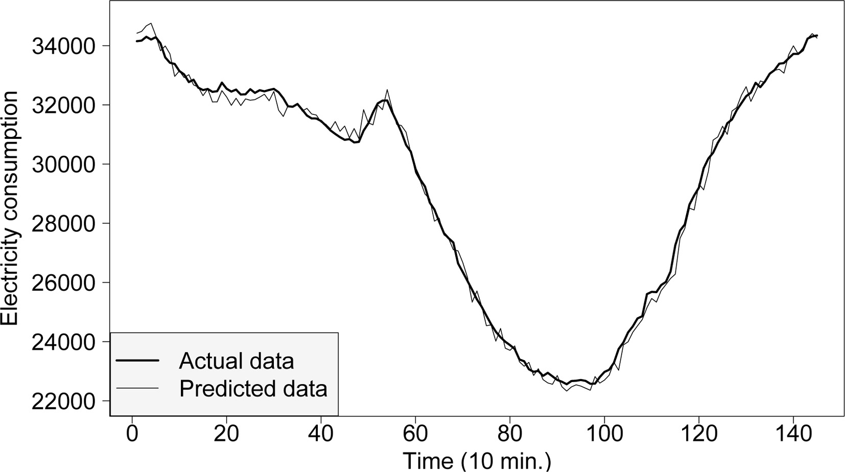

Figure 6.

Worst daily forecast in the test set.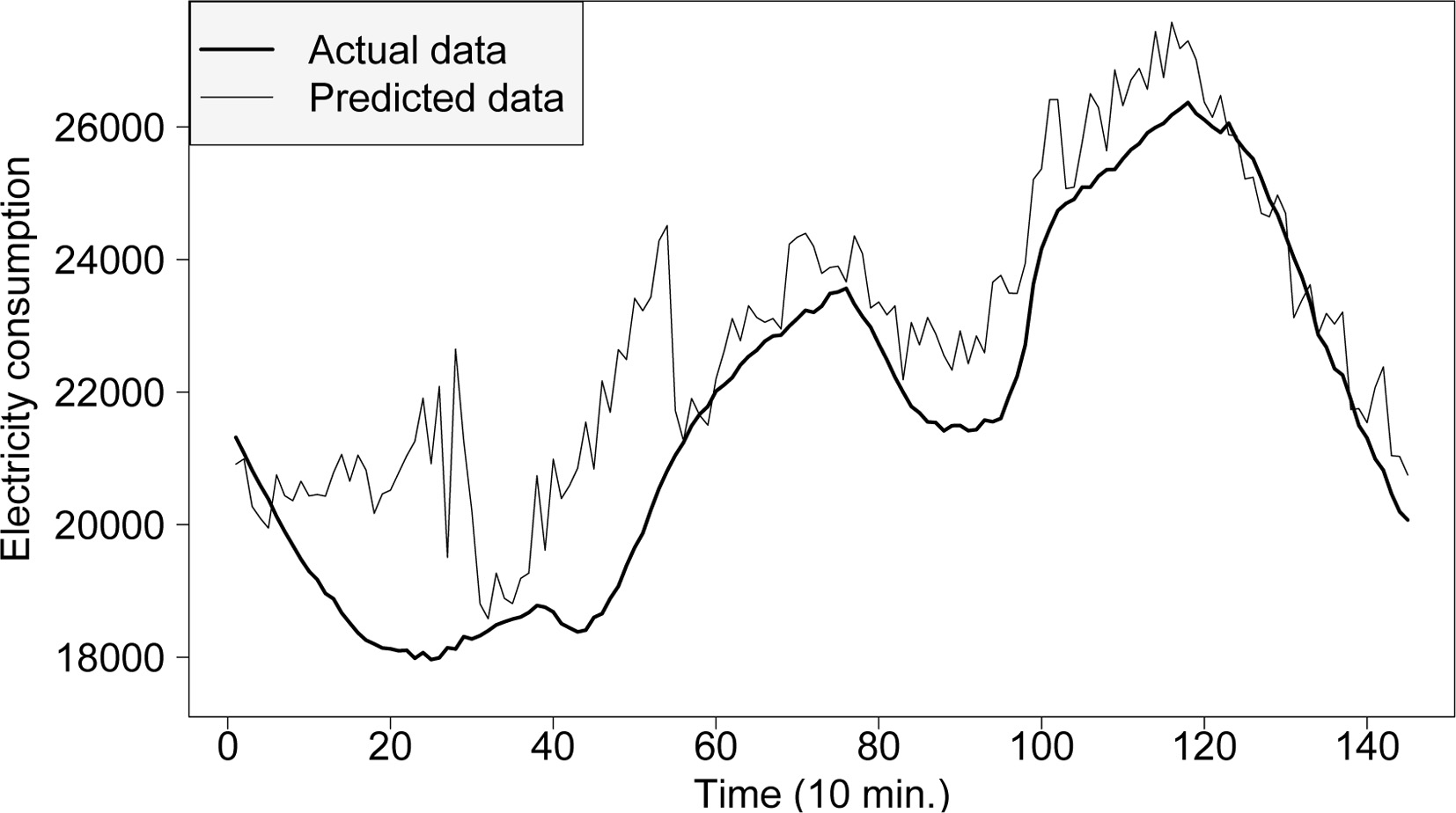

Figure 7.

Daily average of the time series in April and May 2016.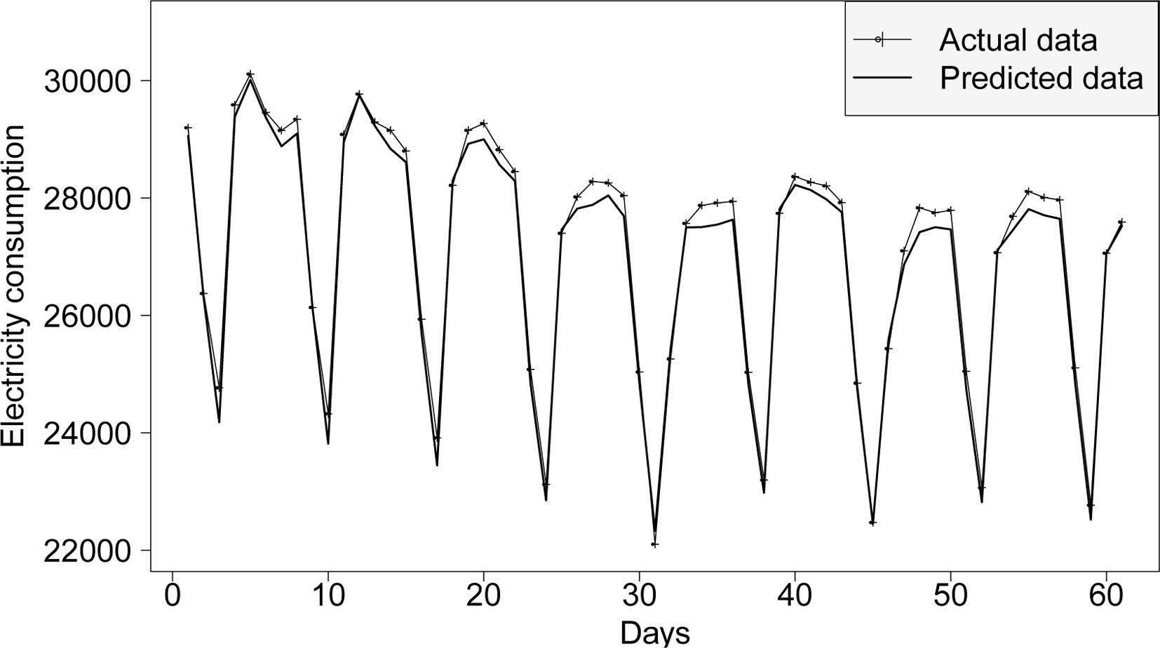

4.4 Scalability

This section presents a study of scalability of the deep neural network proposed to predict very long time series. For that purpose, the deep learning algorithm has been executed for different lengths of the time series and number of execution threads.

Table 4 shows the computing times of the deep neural network for its training phase when varying the number of threads in a single machine from 2 to 12 by steps of 2, and the length of the series increases depending on a multiplicative factor. Thus, x2 stands for a factor of 2, and so forth. In particular, runtimes have been obtained with time series of two, four, eight, sixteen, thirty and two, and sixty and four times the length of the original time series. Figure 8 graphically summarizes the results collected from Table 4. It is noticeable that the deep learning model here proposed for big data time series is scalable as the runtimes increase in a linear way when increasing the size of the dataset. Moreover, it can be seen that the optimal resources for the different sizes of the time series used in this experiment are 6 threads as similar runtimes are provided when using a larger number of threads.

Table 4
Computing times for different lengths and threads

Multiplier	File size	Threads	Training time (sec)
x1	23.9 MB	2	595
		4	327
		6	244
		8	237
		10	232
		12	229
x2	47.8 MB	2	1195
		4	639
		6	464
		8	449
		10	420
		12	384
x4	95.5 MB	2	2389
		4	1284
		6	915
		8	872
		10	802
		12	782
x8	191.1 MB	2	4823
		4	2961
		6	1837
		8	1725
		10	1590
		12	1524
x16	382.2 MB	2	9276
		4	5394
		6	3763
		8	3579
		10	3356
		12	3235
x32	764.4 MB	2	18244
		4	10719
		6	7438
		8	7034
		10	6540
		12	6333
x64	1.5 GB	2	35802
		4	20911
		6	14489
		8	13929
		10	13071
		12	12673

Figure 9a and b present how the runtime in the training phase decreases as the number of threads in a single machine increases. This phenomenon happens independently of the dataset size, but some important issues can be concluded. For instance, the number of threads for a short time series (for instance x1) is not too relevant as the training computing time by using 6, 8, 10 or 12 threads does not show a great improvement. However, the reduction of runtimes is much more remarkable with very long time series (for instance x64) as it can be seen in Fig. 9.

Figure 8.

Computing times versus length of the time series.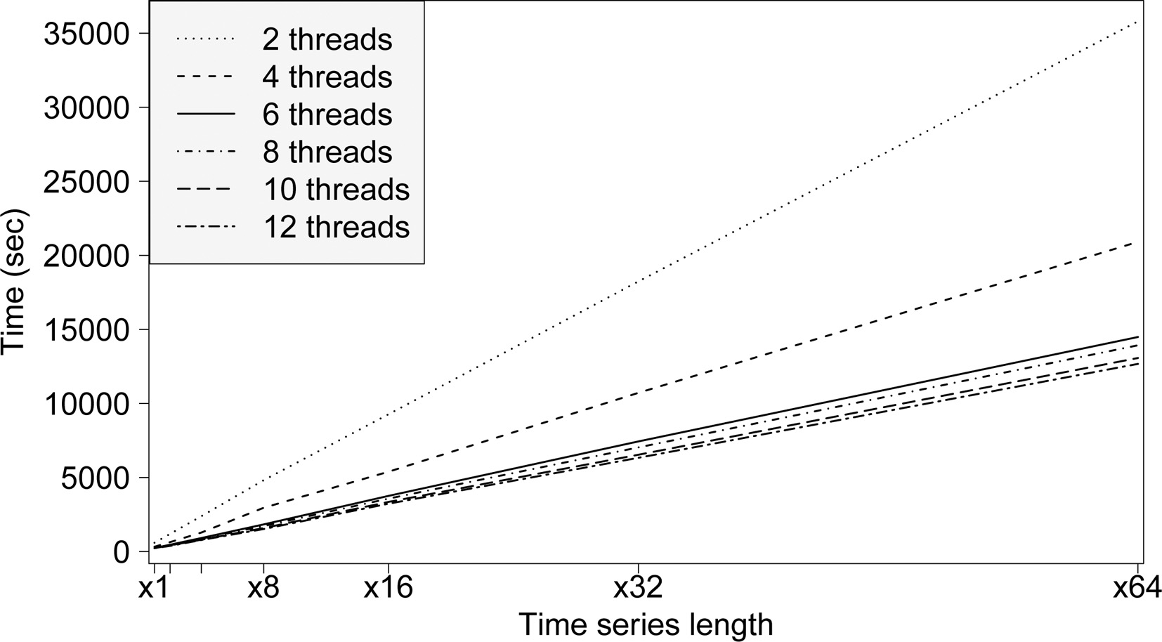

Figure 9.

Computing times depending on the number of threads.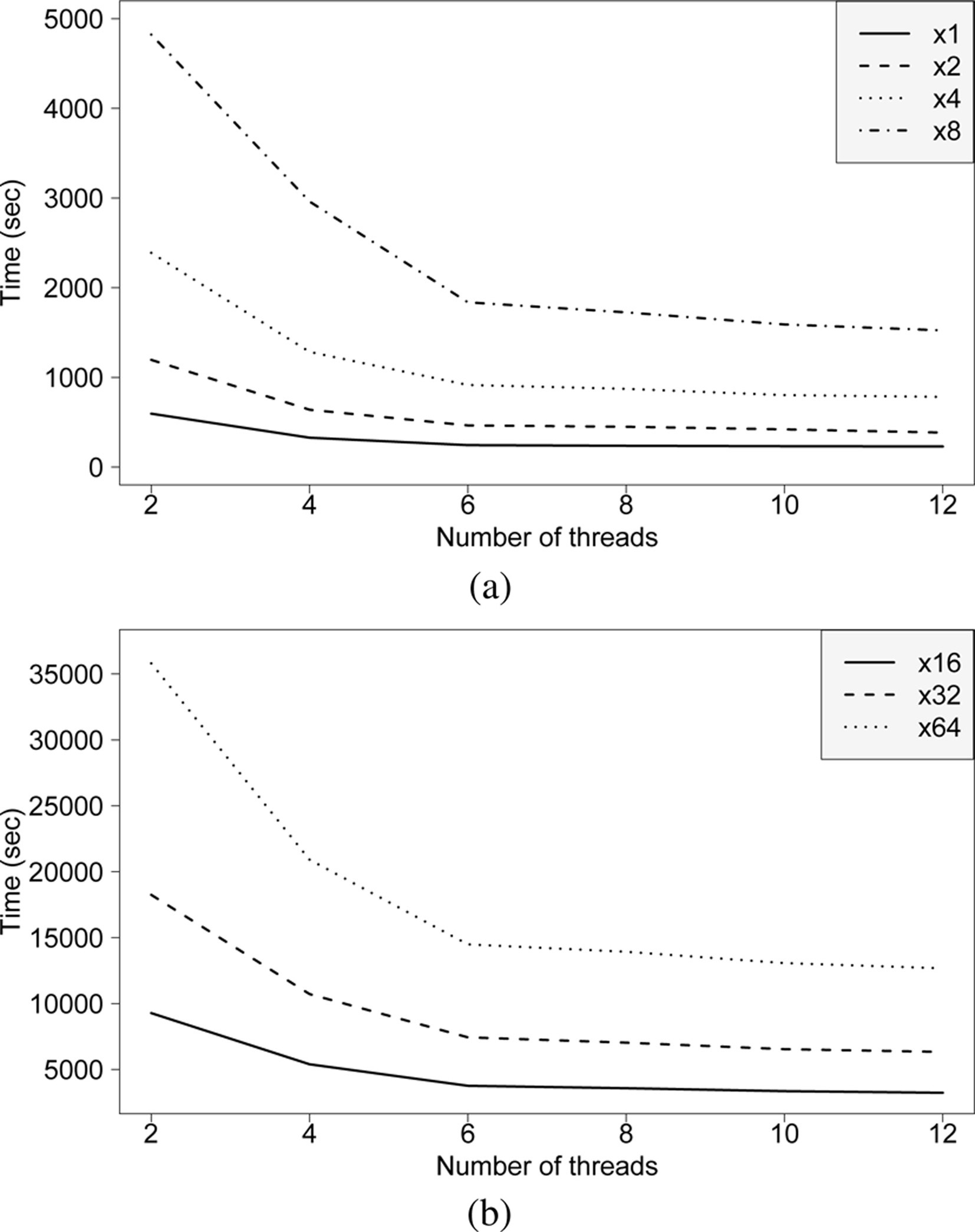

5. Comparative analysis

The proposed deep learning based methodology has been compared to the methods reported in [16], namely, a linear regression (LR), a decision tree (DT) and two ensemble techniques based on trees as Gradient-Boosted Trees (GBT) and Random Forest (RF). The parameters of these methods used in this work were the optimal parameters obtained by a grid search in [16]. Tree-based methods are very common in machine learning, both for classification and for regression, as they are easy to interpret, support continuous and discrete attributes, do not require attribute scaling and are able to model nonlinear relationships between attributes. A brief description of these methods used for the comparison is made below.

LR minimizes the mean square error of the training set by using the well-known stochastic gradient descent method and is usually selected as a reference model.

DT is obtained through a recursive binary partition of the feature space. At each iteration, the attribute chosen to divide the tree is the one that maximizes the information gain. The recursive construction of the tree stops when there are not enough attributes in the child nodes or the maximum depth is reached.

Table 5
Comparison of accuracy and runtimes

Method	MRE (%)	Time (s)
Deep learning	1.6769	153
Linear regression	7.3395	553
Decision tree	2.8783	81
Gradient-boosted trees	2.7190	417
Random forest	2.2005	277

Table 6

MRE for each sub-problem

Sub-problem	DT	GBT	RF	DL
1	1.13	1.11	1.08	0.77
2	1.32	1.30	1.17	1.13
3	1.59	1.54	1.33	1.15
4	1.87	1.82	1.52	1.18
5	2.09	2.02	1.66	1.35
6	2.41	2.32	1.90	1.36
7	2.64	2.54	2.17	1.50
8	2.77	2.66	2-22	1.71
9	2.95	2.86	2.35	1.88
10	3.04	2.88	2.47	1.76
11	3.13	3.00	2.45	1.66
12	3.41	3.23	2.57	2.07
13	3.61	3.32	2.86	1.83
14	3.95	3.60	2.88	1.81
15	3.90	3.58	2.94	2.11
16	3.92	3.59	2.94	1.93
17	3.88	3.52	3.04	2.50
18	4.05	3.79	3.11	2.09
19	3.89	3.65	3.13	2.17
20	3.85	3.63	3.15	2.14
21	3.97	3.85	3.17	2.43
22	3.93	3.76	3.19	2.56
23	4.03	3.84	3.17	2.42
24	4.03	3.83	3.15	2.77

Table 7

Training time for each subproblem in DL method

Sub-problem	Seconds	Sub-problem	Seconds
1	10.86	13	4.33
2	6.36	14	6.42
3	6.36	15	5.31
4	5.36	16	5.35
5	6.34	17	5.34
6	4.36	18	6.34
7	5.31	19	8.37
8	7.32	20	5.34
9	6.35	21	7.47
10	5.35	22	6.32
11	5.39	23	7.38
12	7.35	24	8.32

Ensembles methods are learning algorithms that create a set of basic models to compose the final model. GBT and RF offer very good results for many real applications, showing a high performance in regression tasks and improving the results obtained by a single regression. Both training processes to generate the model are different for each algorithm. In particular, GBT [62] is a set of decision trees trained iteratively. Thus, in each iteration, the algorithm uses the ensemble of trees of the previous iteration to correct the mistakes made in the prediction, thereby improving the accuracy in the following ensemble of trees. On the other hand, RF [63] generates a set of decision trees in parallel. Combining them, the probability of obtaining an overfitted model is reduced. Also, a different training set is used in each tree in order to introduce randomness. In addition, the nodes of each decision tree consider different subsets of attributes. To predict a new instance, RF makes an estimation with the average of the predictions obtained with each tree.

Table 8

Runtimes (expressed in seconds) for different time series lengths

Method	x1	x2	x4	x8	x16	x32	x64
Deep learning	153	218	361	649	1209	2346	4601
Linear regression	553	846	1483	2710	5162	10057	19871
Decision tree	81	120	201	353	653	1329	2644
Gradient-boosted trees	417	581	968	1720	3336	6490	13141
Random forest	277	440	783	1525	3128	6416	12518

Figure 10.

Scalability of the deep learning and all methods used for comparison.

The results obtained of the application of these methods to the time series described in the Section 4.1 were compared in [16], using an Apache Spark cluster with one master and two slaves with Intel Core i7-5820K @ 3.30 GHz processors and 16 GB of memory for each machine. A comparison between the accuracy and runtimes (in seconds) for the deep feed-forward neural network method proposed here by using the cluster described above and the results from [16] is shown in Table 5, where methods are ordered by prediction error for the test set. The deep learning achieves a MRE of 1.6769% for the test set, meaning an improvement of 0.52% compared to RF –the method with the best accuracy from [16]–, 1.20% compared to only one decision tree, and a 5.66% in comparison with the linear regression. These improvements in relation to errors are of significant importance to avoid misalignments in the planning of energy production that would cause large losses.

The errors and computing times desagregated for each subproblem in order to evaluate the performance of each model separately are presented in Tables 6 and 7. It can be appreciated only learning times for Deep Learning are showed in Table 7. This is due to similar computing times for each subproblem are obtained in DT, LR and RF cases, corresponding to times shown in Table 5 divided by 24. However in Deep learning case, each subproblem is solved with a different number of neurons and layers, and therefore, computing times for each are different.

Table 8 and Fig. 10 show a comparison of the training execution times – expressed in seconds – for different time series lengths in order to compare the scalability of the deep learning, LR, DT, GBT and RF. As can be seen in Table 8, the behavior of all methods is the same, keeping a linear scalability factor according to the time series length. Figure 10 represents graphically how training times increase according to the length of the time series. Both tree-ensemble methods improve execution times regarding the linear regression, but definitely deep learning and DT are at a different level, being DT the most scalable method of the comparison, followed closely by the deep learning method.

6. Conclusions

A deep feed forward neural network applied to time series forecasting has been proposed in this work to deal with big data. The Apache Spark distributed computing platform has been used to execute the algorithm in a cluster of machines. The H2O framework has been used for big data analysis, providing the deep learning method here proposed. Reported results have shown that the deep learning configuration setting is important to obtain a good accuracy. A preliminary study of several parameters has been made, obtaining a mean relative error less than a 2%. The scalability of the method has been assessed depending on the time series length and the number of execution threads, showing a linear scalability and a high performance for distributed computing. Finally, the methodology has been compared to other recently published techniques in terms of accuracy and scalability. The deep learning one turned out to be one of the most adequate methods to process big data time series along with decision trees, in terms of scalability, and the best method in terms of accuracy.

Footnotes

Acknowledgment

The authors would like to thank the Spanish Ministry of Economy and Competitiveness and Junta de Andalucía for the support under projects TIN2014- 55894-C2-R, TIN2017-88209-C2-1-R, and P12-TIC-1728, respectively.

References

Rossell

Alomar

Morro

Oliver

Canals

. High-density liquid-state machine circuitry for time-series forecasting. International Journal of Neural Systems. 2016; 26(5): 1-12.

Martínez-Álvarez

Troncoso

Asencio-Cortés

Riquelme

. A survey on data mining techniques applied to energy time series forecasting. Energies. 2015; 8: 1-32.

Adeli

Kumar

. Distributed computer-aided engineering: for analysis, design, and Visualization. 1st ed. Boca Raton, FL, USA: CRC Press, Inc.; 1998.

Adeli

. Parallel processing in computational mechanics. New York, NY, USA: Marcel Dekker, Inc., 1992.

Adeli

Cheng

. Concurrent genetic algorithms for optimization of large structures. 1994 07; 7: 276-296.

Deleforge

Forbes

Horaud

. Acoustic space learning for sound-source separation and localization on binaural manifolds. International Journal of Neural Systems. 2015; 25(1): 1440003.

Donnarumma

Prevete

Chersi

Pezzulo

. A programmer-interpreter neural network architecture for prefrontal cognitive control. International Journal of Neural Systems. 2015; 25(6): 1-16.

Hirschauer

Adeli

Buford

. Computer-aided diagnosis of parkinson’s disease using an enhanced probabilistic neural network. Journal of Medical Systems. 2015; 39(179): 1-12.

Zeinalia

Story

. Competitive probabilistic neural network. Integrated Computer-Aided Engineering. 2017; 24(2): 105-118.

10.

Livingstone

Manallack

Tetko

. Data modelling with neural networks: advantages and limitations. Journal of Computer-Aided Molecular Design. 1997; 11: 135-142.

11.

Sutskever

Martens

Dahl

Hinton

. On the importance of initialization and momentum in deep learning. Proceedings of the International Conference on Machine Learning (ICML), 2013; 1139-1147.

12.

Torres

Fernández

Troncoso

Martínez-Álvarez

. Deep learning-based approach for time series forecasting with application to electricity load. Proceedings of the International Work-Conference on the Interplay Between Natural and Artificial Computation (IWINAC), 2017; 203-212.

13.

Goodfellow

Bengio

Courville

. Deep learning. MIT Press, 2016.

14.

Schmidhuber

. Deep learning in neural networks: An overview. Neural Networks. 2015; 61: 85-117.

15.

Candel

LeDell

Parmar

Arora

. Deep learning with H2O. H2O.ai, Inc.; 2017.

16.

Galicia

Torres

Martínez-Álvarez

Troncoso

. Scalable forecasting techniques applied to big electricity time series. Proceedings of the 14th International Work-Conference on Artificial Neural Networks (IWANN), 2017; 165-175.

17.

Adeli

. Supercomputing in engineering analysis. New York, NY, USA: Marcel Dekker, Inc., 1992.

18.

Castillo

Peteiro-Barral

Berdis

Fontenla-Romero

. Distributed one-class support vector machine. International Journal of Neural Systems. 2015; 25(7): 1550029.

19.

Adeli

Hung

. A concurrent adaptive conjugate gradient learning algorithm on mimd shared-memory machines. The International Journal of Supercomputing Applications. 1993; 7(2): 155-166.

20.

Fang

Zhang

Zhou

Liao

Wang

. Benchmarking the GPU memory at the warp level. Parallel Computing. 2018; 71: 23-41.

21.

Bureddy

Wang

Venkatesh

Potluri

Panda

. OMB-GPU: A micro-benchmark suite for evaluating MPI libraries on GPU clusters. Proceedings of the 19th European MPI Users’ Group Meeting (EuroMPI2012). Berlin, Heidelberg: Springer Berlin Heidelberg; 2012; 110-120.

22.

Jacobs

Dryden

Pearce

Essen

. Towards scalable parallel training of deep neural networks. Proceedings of the Machine Learning on HPC Environments (MLHPC). New York, NY, USA: ACM, 2017; 5:1-5:9.

23.

Ortega-Zamorano

Jerez

Gómez

Franco

. Layer multiplexing FPGA implementation for deep back-propagation Learning. Integrated Computer-Aided Engineering. 2017; 24(2): 171-185.

24.

Dean

, et al. Large scale distributed deep networks. Proceedings of the 25th International Conference on Neural Information Processing Systems (NIPS). USA: Curran Associates Inc.; 2012; 1223-1231.

25.

Reagen

Whatmough

Adolf

Rama

Lee

, et al. Minerva: Enabling low-power, highly-accurate deep neural network accelerators. 2016; 44: 267-278.

26.

Tokui

Oono

Hido

Clayton

. Chainer: A next-generation open source framework for deep learning. Proceedings of Workshop on Machine Learning Systems (LearningSys) in the 29th Annual Conference on Neural Information Processing Systems (NIPS); 2015.

27.

Abadi

, et al. TensorFlow: Large-Scale Machine Learning on Heterogeneous Systems; 2015. Software available from tensorflow.org.

28.

Erickso

Korfiatis

Akkus

Kline

Philbrick

. Toolkits and libraries for deep learning. Journal of Digital Imaging. 2017; 30(4): 400-405.

29.

Martínez-Ballesteros

Bacardit

Troncoso

Riquelme

. Enhancing the scalability of a genetic algorithm to discover quantitative association rules in large-scale datasets. Integrated Computer-Aided Engineering. 2015; 22(1): 21-39.

30.

Martín

Martínez-Ballesteros

García-Gil

Alcalá-Fdez

Riquelme

Herrera

. MRQAR: A generic mapreduce framework to discover quantitative association rules in big data problems. Knowledge-Based Systems. 2018; 153: 176-192.

31.

Romeu

Zamora-Martínez

Botella-Rocamora

Pardo

. Time-series forecasting of indoor temperature using pre-trained deep neural networks. Proceedings of the 23rd International Conference on Artificial Neural Networks (ICANN); 2013; 451-458.

32.

Ding

Zhang

Liu

Duan

. Deep learning for event-driven stock prediction. Proceedings of the International Joint Conference on Artificial Intelligence, 2015; 2327-2334.

33.

Dalto

Matusko

Vasak

. Deep neural networks for ultra-short-term wind forecasting. Proceedings of the IEEE International Conference on Industrial Technology (ICIT), 2015; 1657-1663.

34.

Peng

Shao

Chi

. Deep learning architecture for air quality predictions. Environmental Science and Pollution Research International. 2016; 23: 22408-22417.

35.

Baek

Sohn

. Deep-learning architectures to forecast bus ridership at the stop and stop-to-stop levels for dense and crowded bus networks. Applied Artificial Intelligence. 2016; 30(9): 861-885.

36.

Ortiz

Munilla

Górriz

Ramírez

. Ensembles of deep learning architectures for the early diagnosis of the alzheimer’s disease. International Journal of Neural Systems. 2016; 26(7): 1650025.

37.

Morabito

, et al. Deep learning representation from electroencephalography of early-stage creutzfeldt-jakob disease and features for differentiation from rapidly progressive dementia. International Journal of Neural Systems. 2017; 27(2).

38.

Acharya

Hagiwara

Tan

Adeli

. Deep convolutional neural network for the automated detection and diagnosis of seizure using EEG signals. Computers in Biology and Medicine. 2017; in press.

39.

Wang

Zhang

. An adaptive neural network approach for operator functional state prediction using psychophysiological data. Integrated Computer-Aided Engineering. 2016; 21(1): 81-97.

40.

Lin

Nie

. Structural damage detection with automatic feature-extraction through deep learning. Computer Aided Civil and Infrastructure Engineering. 2017; 32: 1025-1046.

41.

Zhang

Wang

Yang

Dai

, et al. Automated pixel-level pavement crack detection on 3D asphalt surfaces using a deep-learning network: Pixel-level pavement crack detection on 3D asphalt surfaces. Computer-Aided Civil and Infrastructure Engineering. 2017 08; 32.

42.

Cha

Choi

Büyüköztürk

. Deep learning-based crack damage detection using convolutional neural networks. Computer-Aided Civil Infrastructure Engineering. 2017 May; 32(5): 361-378.

43.

Hossein

Adeli

. A novel machine learning based algorithm to detect damage in highrise building structures. The Structural Design of Tall and Special Buildings. 26(18): e1400. E1400 TAL-17-0022.R1.

44.

Rafiei

Adeli

. A novel unsupervised deep learning model for global and local health condition assessment of structures. Engineering Structures. 2018; 156: 598-607.

45.

Koziarski

Cyganek

. Image recognition with deep neural networks in presence of noise – Dealing with and taking advantage of distortions. Integrated Computer-Aided Engineering. 2017; 24(4): 337-349.

46.

Rigos

Tsekouras

Vousdoukas

Chatzipavlis

Velegrakis

. Chebyshev polynomial radial basis function neural network for automated shoreline extraction from coastal imagery. Integrated Computer-Aided Engineering. 2016; 23(2): 141-160.

47.

Coelho

da S Luz

Ochi

Guimars

Rios

. A GPU deep learning metaheuristic based model for time series forecasting. Applied Energy. 2017; 201: 412-418.

48.

Rafiei

Adeli

. A novel machine learning model for estimation of sale prices of real estate units. Journal of Construction Engineering and Management. 2016; 142(2): 04015066.

49.

Kuremoto

Kimura

Kobayashi

Obayashi

. Time series forecasting using a deep belief network with restricted Boltzmann machines. Neurocomputing. 2014; 137: 47-56.

50.

. Electricity consumption prediction using a neural-network-based grey forecasting approach. Journal of the Operational Research Society. 2016; 68(10): 1259-1264.

51.

Marvuglia

Messineo

. Using recurrent artificial neural networks to forecast household electricity consumption. Energy Procedia. 2012; 14: 45-55.

52.

Talavera-Llames

Pérez-Chacón

Martínez-Ballesteros

Troncoso

Martínez-Álvarez

. A nearest neighbours-based algorithm for big time series data forecasting. Proceedings of the 11th International ConferenceHybrid Artificial Intelligent Systems (HAIS); 2016; 174-185.

53.

Zaharia

Chowdhury

Franklin

Shenker

Stoica

. Spark: cluster computing withworking sets. Proceedings of the International Conference on Hot Topics in Cloud Computing (ICWS), 2010; 1-10.

54.

Pérez-Chacón

Talavera-Llames

Troncoso

Martínez-Álvarez

. Finding electric energy consumption patterns in big time series data. Proceedings of the International Conference on Distributed Computing and Artificial Intelligence (DCAI), 2016; 231-238.

55.

Grolinger

L’Heureux

Capretz

MAM

Seewald

. Energy forecasting for event venues: Big data and prediction accuracy. Energy and Buildings. 2016; 112: 222-233.

56.

Mocanu

Nguyen

Gibescu

Kling

. Deep learning for estimating building energy consumption. Sustainable Energy, Grids and Networks. 2016; 6: 91-99.

57.

Zhang

Yang

Chen

. A survey on deep learning for big data. Information Fusion. 2018; 42: 146-157.

58.

Brunetti

Buongiorno

Trotta

Bevilacqua

. Computer vision and deep learning techniques for pedestrian detection and tracking: A survey. Neurocomputing. 2018; 300: 17-33.

59.

Litjens

Kooi

Bejnordi

Setio

AAA

Ciompi

Ghafoorian

, et al. A survey on deep learning in medical image analysis. Medical Image Analysis. 2017; 42: 60-88.

60.

Cook

. Practical machine learning with H2O: powerful, scalable techniques for deep learning and AI. O’Reilly Media, 2016.

61.

Arora

Candel

Lanford

LeDell

Parmar

. Deep Learning with H2O. 2015.

62.

Mason

Baxter

Bartlett

Frean

. Boosting algorithms as gradient descent. Proceedings of the Neural Information Processing Systems Conference (NIPS), 1999; 512-518.

63.

Breiman

. Random forests. Machine Learning. 2001; 45(1): 5-32.

A scalable approach based on deep learning for big data time series forecasting

Abstract

Keywords

1. Introduction

3. Methodology

3.1 Theoretical background

4.1 Dataset description

4.2 Design of experiments

Table 1 MRE depending on the historical data window

Table 2 Errors for different lambda and distribution functions

Table 4 Computing times for different lengths and threads

Table 5 Comparison of accuracy and runtimes

Footnotes

Acknowledgment

References

Table 1
MRE depending on the historical data window

Table 2
Errors for different lambda and distribution functions

Table 4
Computing times for different lengths and threads

Table 5
Comparison of accuracy and runtimes