Determining geostrophic wind direction in a rainfall forecast expert system

Abstract

This paper provides a novel method to design a Rainfall Forecasting System based on Neural Networks and a long-term data registry. The System proposed is based on the observations of expert meteorologists after 40 years of research developing local forecast methodologies to predict rainfall events in the Meteorological Observatory of Valladolid, Spain. The Geostrophic Wind, a theoretical value resulting of the balance between the Pressure Gradient Force and the Coriolis Force, is the key parameter which feeds the aforementioned System. The paper focuses on the Geostrophic Wind calculation. We propose a novel method to estimate its direction and magnitude on a local scale, by processing a set of pressure and temperature observations surrounding a central location. This study continues previous research, providing complementary criteria for numerical weather prediction systems based on time-series forecasting and neural networks.

Keywords

Rainfall forecast neural network wavelets multispectral analysis

1. Introduction

Nowadays a significant effort is being made in meteorological research to provide better, more accurate weather forecasts. Weather predictions are provided by Ensemble Prediction Systems (EPS). An ensemble is a collection of weather forecasts, i.e. a set of numerical weather prediction (NWP) systems. Ensembles run the models various times from slightly different, initial conditions. Often the model is also slightly perturbed, and some ensembles use more than one model within said ensemble (multi-model EPS), or the same model with different combinations of physical parameterization schemes (multi-physics EPS), [1]. Some of the most important European reference centers are HIRLAM, ECMWF and the UK MET Office. The European Centre for Medium-Range Weather Forecasts (ECMWF) is supported by 34 states; it is specialized in medium-range forecasts (up to two weeks in advance). HIRLAM (High Resolution Limited Area Model) is a research consortium of European meteorological institutes, which provide a numerical short-range weather forecast, based on a hydrostatic model. The main handicap of medium and long-term forecasts is the uncertainty, either in the measurements or in the model definition, makes the temporal simulation diverge from the real evolution [2, 3, 4].

Since Richardson performed the first NWP setting the equations of a particle in the atmosphere in 1922, prediction systems have evolved remarkably, but have an inherent limitation due to the chaotic nature of the weather itself. With regard to this matter, the need to evolve current forecasting systems to overcome these limitations has been stated [5]. The use of Artificial Neural Networks (ANN) in weather forecasting was first proposed in [6] and during recent years, several authors have made varying approximations to this subject. In [7] an accurate summary of Rainfall prediction, using ANNs, is clearly explained. On the other hand, there are some examples of Expert Systems for weather forecasting [8]. In [9] an interesting summary of Expert system forecasting accuracy is presented; [10] can be an example of representative Expert Systems architecture. Regarding weather time series estimation, [11] presents a time series analysis study on wind estimation and in [12] autoregressive Neural Networks has been applied. Nowadays, the use of Neural systems based on wavelets and multi-scale analysis is becoming more and more popular [13, 14, 15]. This paper continues a study which was started in 2008 [16, 17]. The said study proposes a framework for a local rainfall forecast based on weather time series analysis and neural networks [18], to complement current ensemble predictions. It expands on previous studies which focused on implementing the Rainfall Forecast design to a real time working system. Frequently, data acquisition and filtering is the real endeavor of this type of study since data is not always as clean or available as provided in off-line records.

This paper focuses on the Geostrophic Winds (GW) determination, as it is the most important input to this overall Rainfall prediction system. The GW is defined under hydrostatic equilibrium, without acceleration and friction; therefore its trajectory can only be rectilinear. It is actually a theoretical wind with very restrictive conditions. The GW cannot be directly measured. The GW computation is mainly influenced by reduction of the pressure to mean sea level, systematic biases and random noise in the barometer data, etc. In [19, 20] it is claimed that sometimes in certain places, surface GW cannot be accurately modeled by mean sea level reduction; this is well explained in [21]. An exhaustive study is carried out on the GW in the Gulf of Mexico, in which the seasonal variation of the differences between real and geostrophic wind is characterized with great precision, presented in [22].

The challenge of the study is to obtain the GW in real time from observable and easy-access data. It requires pressure and temperature data, which can be obtained by national meteorological agencies, or can be directly obtained through a meteorological station. Also, the system must be able to deal with the calculation limitations previously mentioned.

The study consists of five parts:

•
Abstract.
•
Section 1: Introduction to the paper.
•
Section 2: Summary of the Rainfall Forecast Model and explanation of the need to obtain the GW direction.
•
Section 3: Proposal of how to obtain the GW.
•
Section 4: A fourth part implementing a GW estimator and evaluating it.
•
Section 5: A conclusion summarizing the key points of the research.

2. Local rainfall forecast design

2.1 Local rainfall forecast model

Over a period of several years in the Meteorological observatory of Valladolid, Spain, expert meteorologists have been observing the repetition of rainfall patterns. To characterize such rainfall events, as an aid to the ensemble prediction, a selected set of data was registered twice a day. The rainfall events produced in Valladolid, surface winds, height winds, pressure, Geopotential and 500–1000 hPa thickness were recorded in a time series for over a decade. A first data analysis showed the high dependence of rainfall events and precipitation amount, with the combination of surface and high altitude winds.

Secondly, it was found that the pressure wave’s evolution might predict frontal and rainfall situations. This set of data trends has been used as an aid to such predictions. The aim of the system is to automate the process and, in a given time frame, being able to predict the trend of data by using historical data and a Neural Networks stage. The system retrieves the pressure and geostrophic wind data from the Spanish Meteorological Agency, which in turn are filtered to make a forecast of such variable trends with the historical database. The data is filtered using a multi-resolution Wavelet filter in order to perform a decomposition of the time series. The filter is designed to simplify and extract the useful information with two objectives:

•
Obtain simple data where rainfall information is contained.
•
Obtain simple time series easy to forecast.

Regarding Wavelet theory and applications, see [23, 24, 25]. The stages of the system, as shown in Fig. 1, are:

•
Capture stage, retrieving input observations.
•
Filtering stage, preparing data.
•
Historical database.
•
Time series forecaster to predict the trend.
•
Classification stage that uses the forecast to estimate rainfall probability with different time horizons.

2.2 Vertical profile of the atmosphere observation time series

As mentioned previously, two sets of variables were selected. The first related to the height between certain pressure levels:

Figure 1.

Local rainfall system architecture.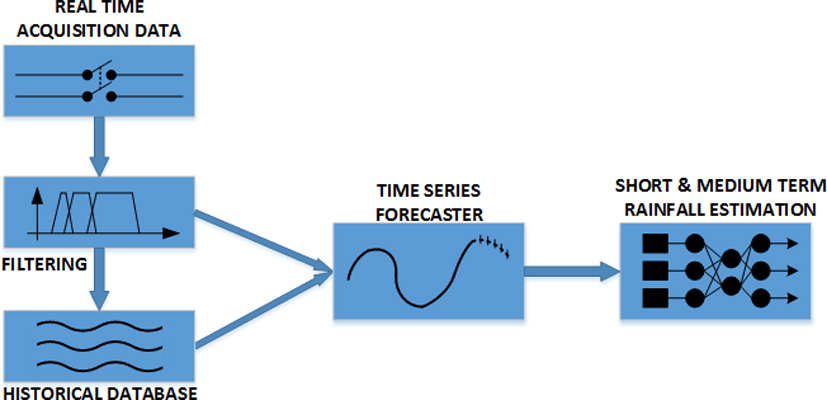

•

Pressure waves, measured in hectopascals, hPa.

•

Geopotential height at 500 hPa, measured in meters.

•

Thickness of the pressure layer from 500–1000 hPa, measured in meters.

Plotting these variables during a certain time frame produces a set of time series, which can be seen as the trend of the vertical profile of the atmosphere. The trend of data shows warm and cold fronts passing through, and other atmospheric situations. These are directly related to rainfall events.

2.3 Geostrophic wind direction observations

To complete the input dataset, the direction of the geostrophic winds (GW) at sea level and at 500 hPa has been registered.

The GW is the resulting wind in the atmosphere under horizontal and hydrostatic movement without any acceleration or friction [26]. GW is the first approximation of the real wind in the atmosphere above the troposphere layer. The GW direction can be obtained from the synoptic charts since they are parallel to isobars; furthermore the magnitude of GW can be obtained from the equilibrium of forces formulation.

Figure 2.

Rainfall occurrence histogram vs Geostrophic Wind combinations. X-axis shows the possible direction of Geostrophic Wind at surface (Wind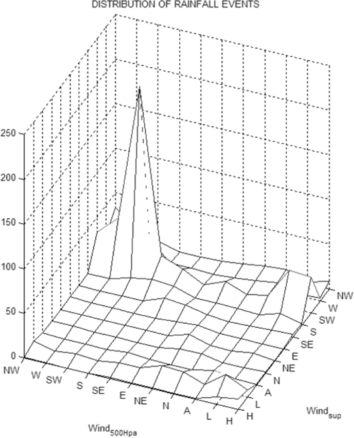 ${}_{\rm sup}$ ), Y axis shows the direction of the Geostrophic Wind at 500 hPa (Wind ${}_{\rm 500Hpa}$ ).

Figure 3.

Rainfall discrete probability density obtained from the GW directions calculated from 1999 to 2006 at Valladolid (Spain). Given the Geostrophic Wind at surface (Wind ${}_{\rm sup}$ ) and the Geostrophic Wind at 500 hPa (Wind500 ${}_{\rm Hpa}$ ), the rainfall probability can be obtained from this plot.

The possible geostrophic wind directions are: North (N), North East (NE), East (E), South East (SE), South (S), South West (SW), West (W), North West (NW), Horse (H), Anticyclone (A) and Cyclones (L). By obtaining rainfall events and intensity histograms, it can be seen that there are some privileged combinations in the direction of winds, both in surface and height, which present a higher probability of precipitation. Figure 2 shows the histogram of the rainfall occurrence depending on the combination of the direction of the geostrophic wind in surface and height.

For each GW couple (surface GW direction and height GW direction), dividing the number of rainy days by the total number of days, provides a discrete probability density function, as shown in Fig. 3.

Figure 4.

Rainfall Probability due Geostrophic Winds and rainfall events in Valladolid during the first 100 days of 1999. The X axis represents time in 12-hour intervals.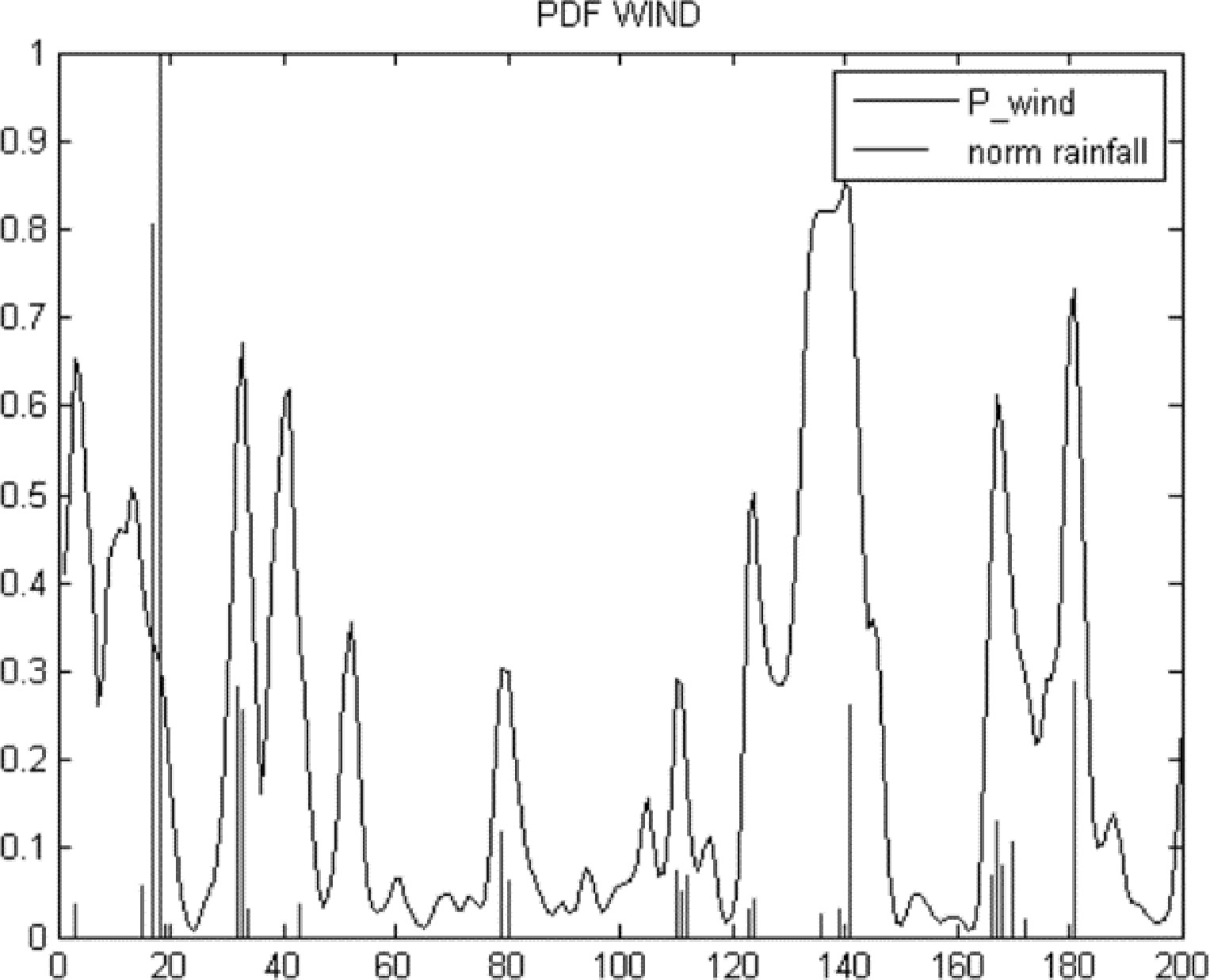

As geostrophic winds (GW) have been registered every 12 hours, this provided a time series that estimates rainfall probability, named P_wind. Figure 4 shows this time series for the beginning of the year 1999. It represents both P_wind and rainfall events which occurred. P_wind peaks enclose rainfall clusters.

Not only does the histogram information clearly show the dependence of GW in rainfall events, but it is also stated that in the feature selection stage – described in [17], – that there is the need for real time GW determination to develop the rainfall forecast system.

3. Geostrophic winds determination

This section summarizes how the Geostrophic Wind directions have been obtained.

3.1 Geostrophic wind description

Even though the concept of GW has been introduced in Section 2.3, a suitable explanation is given to developing this point. The GW is the horizontal equilibrium wind (Vg), blowing parallel to isobars, calculated from the hydrostatic balance between the horizontal pressure gradient force and the Coriolis force. Being in equilibrium, there are no accelerations; therefore the wind moves at a constant speed in a straight line. Equation (1) is the vector formula for the GW:

$\displaystyle V_{g}=\frac{1}{\rho f}\vec{k}\times\mathrm{\nabla}p$ (1)

Being:

•

$f$ , Coriolis Force.

•

$\rho$ , air density [kg/m ${}^{3}$ ].

•

$\vec{k}$ , vertical unity vector.

•

$\mathrm{\nabla}p$ the horizontal gradient of the pressure.

In the POWER project summary [27], it is explained how the GW wind direction and power are obtained using spatial interpolation; on the other hand, in [28] a mean filtering of time series to remove the bias of station measurements has been proposed. The GW calculation is automatically performed by supercomputer centers. The focus in this paper is different: to provide a real time local GW measurement at a particular point. The second challenge is how to assess the obtained measurements.

This paper proposes GW processing in a local area optimizing the gradient estimation (“zone gradients”). Both [29, 30] present state of the art summaries about real wind estimation methods. In [30]some regional solutions in wind estimation are explained.

3.2 Geostrophic winds manual determination in the original dataset

As previously stated, GW has been manually estimated to create the original offline dataset. Every day, twice a day, for more than a decade, the direction of wind was recorded by observing the isobar map provided by the Spanish Meteorological Agency. Note: a GW is named due to the direction in which the wind is blowing. Given a map, the GW origin is obtained parallel to isobars; high pressures are on the right side (in the Northern Hemisphere). Figure 5 shows an isobar map over Spain and the estimated GW direction drawn over it.

3.3 Surface grid surrounding valladolid (Spain)

In order to determine the GW direction, a grid of locations surrounding Valladolid was defined. Figure 6 shows the selected grid of observatories to retrieve pressure.

Table 1
MSL reduced pressures at the stations as obtained in the example of Fig. 5. Each cell of the table represents the MSL in a location of the grid

1019.21	1021.64	1019.20
1020.62	1020.13	1021.33
1022.38	1022.70	1021.56

Figure 5.

Surface synoptic map of Spain taken from NOAA the 21st of October 2017. GW comes from the West. The arrow shows the direction parallel to the isobars; high pressures are on the right-hand side.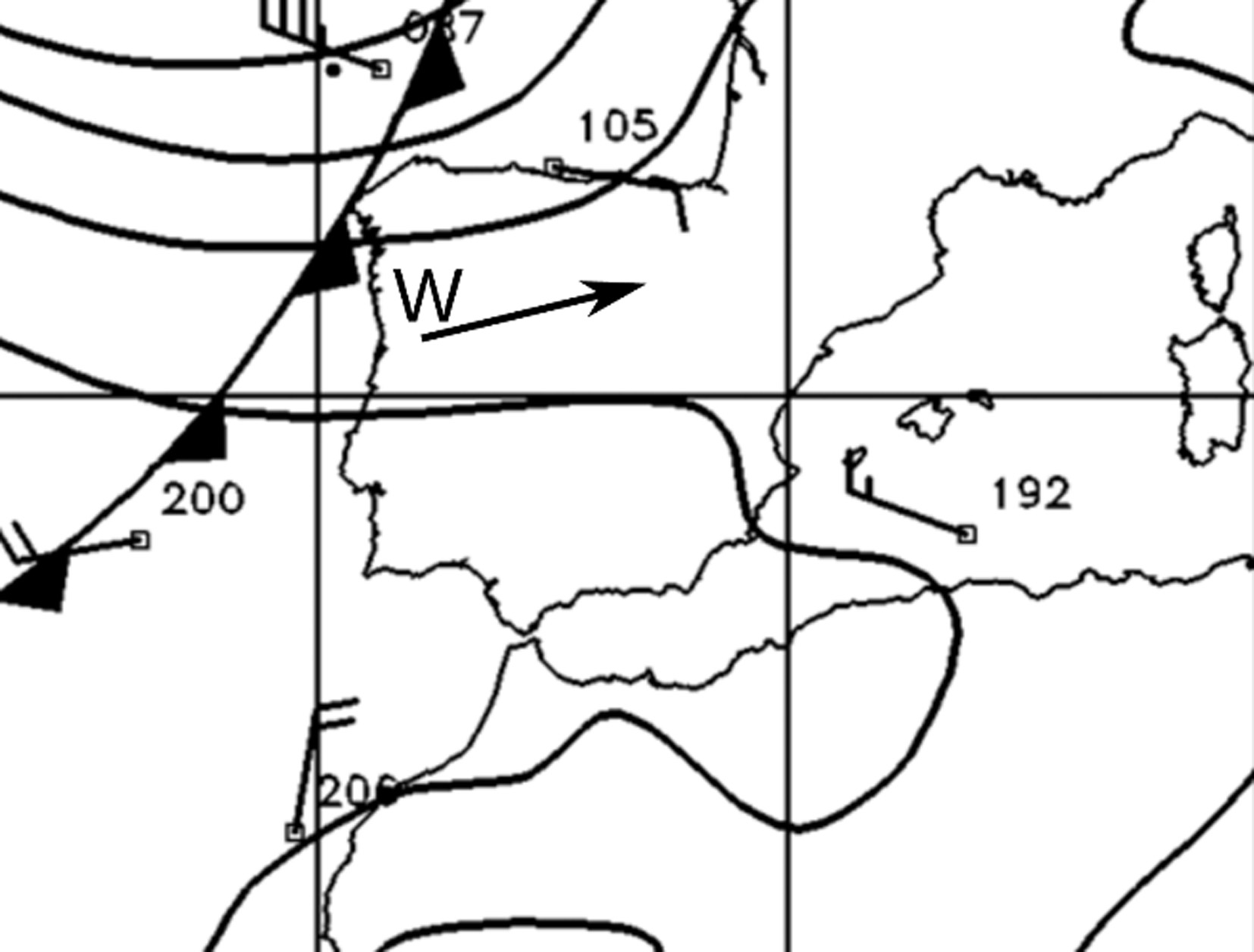

The stations are named as follows in clockwise order:

•

N, Carrión de los Condes.

•

NE, Burgos.

•

E, Aranda de Duero.

•

SE, Guadalajara.

•

S, Talavera.

•

SW, Salamanca.

•

W, Zamora.

•

NW, Ponferrada.

As observed, the NW observatory is further away than the others; since the observatories were selected at similar heights, once the model worked the location was maintained.

3.4 Mean sea level pressure reduction

To compare pressure of different stations it is necessary to reduce the pressure to mean sea level. This subject has been long studied. One of the most useful approximations is the Hypsometric reduction, in Eq. (4) [31]. Being:

•
$P$ , mean sea level reduced pressure.
•
$P_{0}$ , observed pressure.
•
$T$ , temperature.
•
$g$ , constant of gravity $=$ 9.81 m/s ${}^{2}$ .
•
$h$ , height in meters.
•
$\gamma={dT}/{dh}$ , constant temperature variation with height, in K/m.
•
$R_{d}$ , specific gas constant of dry air, in J/K Kg.

$\displaystyle P\left(P_{0},t,h\right)=P_{0}\left(1+\frac{\gamma h}{T-\gamma h}% \right)^{\frac{-g}{{\gamma R}_{d}}}$ (2)

Figure 6.
Grid of pressure stations surrounding Valladolid selected to obtain the data. Each circle represents a location; lines depict the connection to Valladolid, at the center.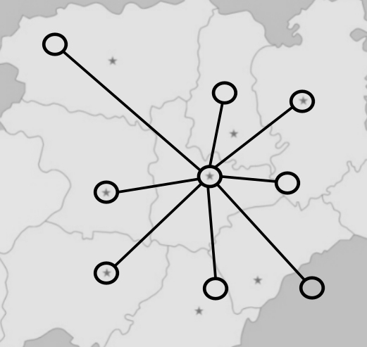

Figure 7.
Observed (left) and Reduced to Sea level (right) pressure over the grid surrounding Valladolid shown in Fig. 6. The observed pressure is reduced to MSL using the hypsometric formula.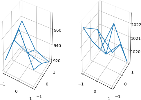

The reduced pressures in the grid of stations for the example in Fig. 5 are shown in Table 1.

Figure 7 shows the observed (left) and reduced (right) pressures of the example in Fig. 5. The bias and noise of the stations produced inaccurate GW calculations (as explained in bibliography). In order to remove the pressure bias of each station, the average of the pressure time series in such stations was subtracted, as suggested in [28]. This process did not produce satisfactory results.
3.5 Grid pressure average gradients

From the data processed by reducing the pressure, some conclusions were obtained:

•
The values of reduced pressure were close to those observed in the maps.
•
The GW direction, directly obtained by the gradient, gave non-accurate values.
•
The preliminary pressure surfaces presented irregular aspect (right section of Fig. 7) but outlines the GW direction.

To improve GW measurements, a spatial average of all gradients along the wind direction in the stations grid was performed. Note, from the definition of GW, high pressures are placed on the right-hand side of the isobars. In addition, the GW must be rectilinear. This is a simple concept, the “Zone Gradient” (ZG), an average of all the contributions at the point justified, as the wind must be rectilinear. To understand how to compute the zone gradient at each point there are two graphical examples.

Figure 8.
(Left) Pressure distribution when the GW blows from the west. (Right) Pressure distribution when the GW blows from the northwest.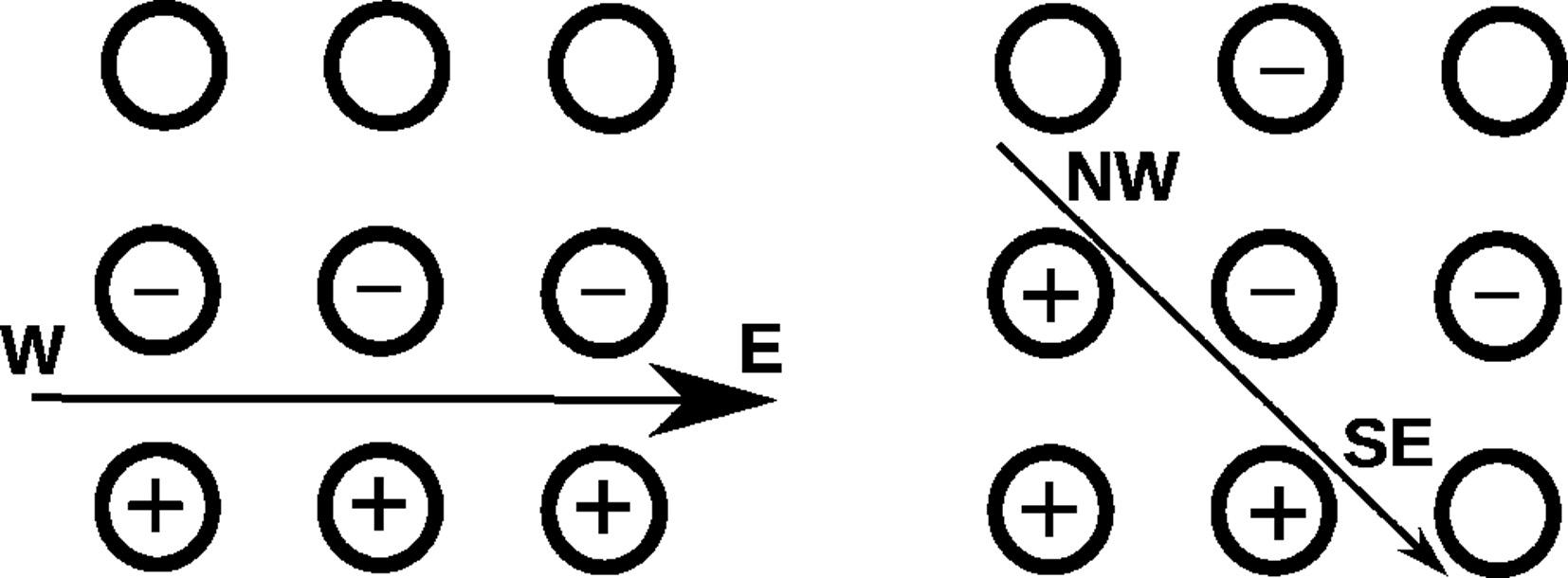

3.5.1 Zone gradient west component point

The wind blowing from the west leaves the high pressures in the south; this is represented in the left-hand diagram in Fig. 8. The ZG of the west is the average of three gradients:

•
From Salamanca to Zamora.
•
From Talavera to Valladolid.
•
From Guadalajara to Aranda.

3.5.2 Zone gradient north-west component point

The wind blowing from the northwest leaves the high pressures as represented on the right-hand side of Fig. 8. The ZG of the west is the average of three gradients:

•
From Zamora to Carrion.
•
From Salamanca to Valladolid.
•
From Talavera to Aranda.

Figure 9.
(Left) Preliminary GW surface, 21/10/2017. Each point of the surface have been obtained computing an average of gradients. (Right) Resulting plane after fit. This figure actually represents a pressure surface with the wind coming from the west.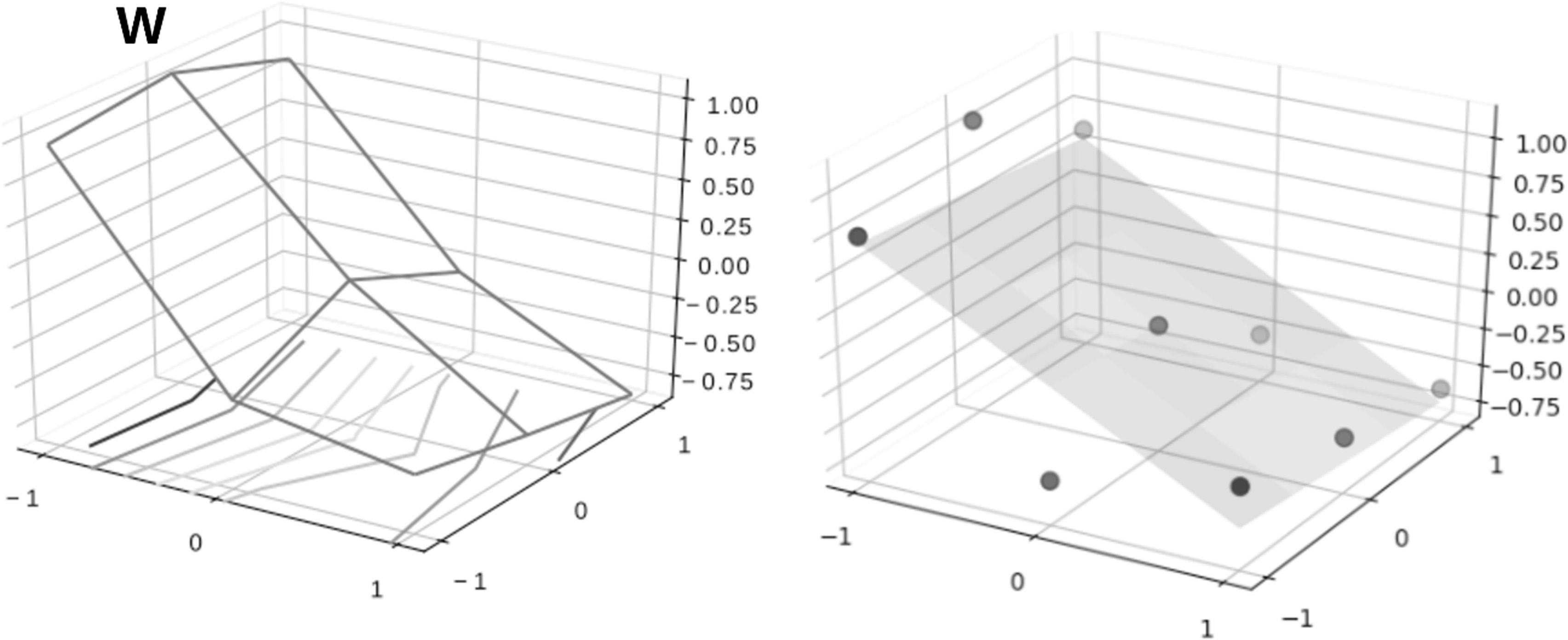

Figure 10.
GW Estimator Architecture. The weights W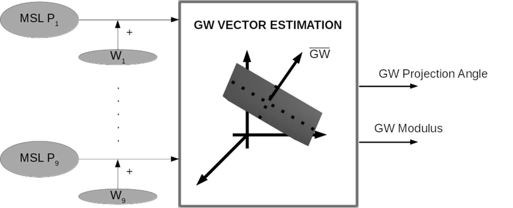 ${}_{i}$ correct the bias of the system optimizing the GW estimation. The weights are obtained minimizing the Mean Square Error of a set of observations. In this study, the data retrieved during a three-month period were used to fit the estimator.

3.5.3 Preliminary surface representation

Every ZG point obtained as explained can be represented in the (3 $\times$ 3) grid. This produces a figure which represents an estimation of the pressure surface. The left section of Fig. 9 shows the resulting surface indicating that GW blows from the west. Note this surface corresponds to Fig. 5, October 21st 2017.

3.5.4 Pressure surface fit, GW direction and module calculation

Although the preliminary surface obtained outlines GW direction, the resulting surfaces may present an irregular aspect. On the other hand, the only way to measure the classifier accuracy was to obtain an estimation of the GW direction. Obtaining the plane that best fits the grid of 9 points solves this problem; this is an approximation to the gradient surface. Obtaining the plane that is most suited, is a trivial least-squares estimation of the plane Z expressed in the following way:

$\displaystyle Z=A*X+B*Y+C$ (3)

The solution of the system consists of minimizing the error function:

$\displaystyle E\left(A,B,C\right)=\sum\nolimits_{n=1}^{n}\left(\left(Ax_{i}+By% _{i}+C\right)-z_{i}\right)$ (4)

The resulting GW estimation, $|\overline{V_{E}}|$ , would be the normal vector of the plane:

$\displaystyle\left|\overline{V_{E}}\right|=\langle A,B,-1\rangle$ (5)

The direction $\Phi$ of the GW would be the projection over the horizontal plane. This is the inverse tangent of $-B/A$ :

$\mathrm{\Phi}=\tan^{-1}\left(\frac{-B}{A}\right)$ (6)

Note the minus sign comes to keep the wind direction sense (the origin point). The angles follow the radians convention:

Figure 11.

Sometimes it is not possible to estimate a GW direction from a map. This map shows a Low-pressure cyclone in the south of Spain and the isobars are open. There is no GW or cannot be guessed correctly.

Figure 12.

Left figure shows the error in the training samples after optimization. Right figure shows the Histogram of the error obtained. Error is expressed in degrees. This figures shows how the estimator works with the training data.

Figure 13.

Error in verification samples (left) and resulting error histogram in the verification (right). Error is expressed in degrees. Note, the error in the verification dataset is the error of the system. Finally a MSE of 15 degrees was obtained.

•

Positive angles, counter-clockwise, from (0, $\pi$ ) radians or (0, 180) degrees.

•

Negative angles, clockwise, from (0, $-\pi$ ) radians or (0, 180) degrees.

The right section of Fig. 9 shows the resulting plane for the studied situation in Fig. 5, the obtained angle was 4 degrees, a wind blowing from the West.

Regarding the GW magnitude it should be proportional to the modulus of normal vector surface; in other words, the scalar product of the proposed WG estimation should be proportional to the actual WG, $|\overline{V_{g}}|$ . This can be written as:

$\displaystyle\left|\overline{V_{g}}\right|=K\left|\overline{V_{E}}\right|=K% \sqrt{\overline{V_{E}}\overline{V_{E}}}$ (7)

The ${\rm K}$ constant has been determined experimentally.

4. Geostrophic winds estimator

This section explains how to effectively perform a GW estimator based on the former section development and the results evaluation. To implement the estimator, some steps have been followed:

•
Estimator design.
•
Training vectors preparation.
•
GW direction estimation fit. GW speed interpolation fit.
•
Results evaluation.

4.1 Estimator design

The system design implements a bias correction to the input Mean Sea Level pressures. The proposed architecture is represented in Fig. 10. The inputs to the system are the reduced pressures of the meteorological stations (MSL ${\rm P}_{\rm i}$ ) and the correction biases ( ${\rm W}_{\rm i}$ ). The aim is to find the optimal set of biases to minimize the Mean Square Error.

4.2 Training vectors preparation

The preparation of the training vectors consisted of measuring the angle of the GW from the synoptic maps automatically retrieved daily. The study started using the National Oceanic and Atmospheric Administration (NOAA) maps but some events evolved the process:

•
NOAA maps do not provide a scale to estimate the force of the GW.

•
In addition, on occasion the original maps cannot provide the GW direction, usually with Cyclones, Anticyclones and Barometric Horses configurations. Figure 11 shows an example of such situations.
•
To minimize error, the synoptic maps from three different sources were analysed for every sample. Using the average of all measurements as the target direction of the wind.
•
Furthermore, a significant number of days are retrieved with missing data due to lack of availability of some stations. These samples cannot be processed.

The vectors were divided into a training set ( $n=$ 70) and a verification set ( $n=$ 20). The training vectors were used to fit biases of the estimator; the verification set to check the performance.

Figure 14.
Left, MET Office winds speed scale in knots. Right, the value of the Geostrophic Winds speed is retrieved from MET Office map calculating the distance between isobars, 22/02/2018.

Figure 15.
GW speed estimation vs. measured speed in knots from training data.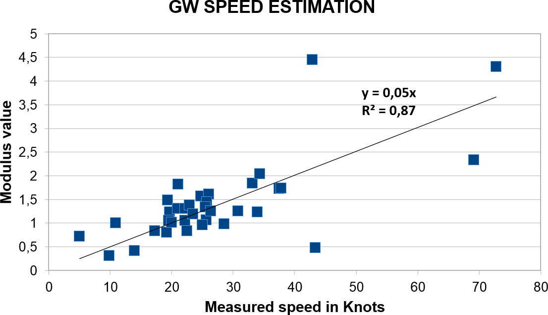

4.3 Angle estimator optimization

In order to adjust the weights of the proposed estimator, a gradient descent algorithm was implemented. It minimized the MSE of the angle estimation in the Training Dataset. After some iteration, the MSE was reduced to 11 degrees per sample. This weight adjustment was then checked with the Verification Dataset, in which a MSE of 15.07 degrees was obtained.

The estimation error in the Training Dataset is shown in the left image of Fig. 12. The right picture shows the histogram of the error. Verification results are shown in Fig. 13 (errors and histogram). The verification results present good performance yet they may be of limited accuracy; the input vectors are obtained manually and sometimes subjected to interpretation. This manual process is suitable as a first step but may be optimized.

4.4 Modulus estimator

As explained previously, the magnitude of the GW should be proportional to the pressure surface normal vector. To evaluate this, the magnitude of the actual GW was obtained from the UK MET Office maps. For each map the distance between isobars was measured and then translated to knots speed using the map scale. The left section of Fig. 14 shows the MET Office wind speed scale placed in the synoptic charts. Note that measuring the distances between isobars on a map is a non-repetitive task and subject to error. Such measurements must be understood as approximations. The right side of Fig. 14 shows how the speed of GW has been acquired. Plotting the estimation of the GW modulus versus the measurements of the synoptic maps produced Fig. 15. The figure provides some important data:

•
The fit follows the expected linear behaviour of Eq. (7): K $=$ 0.05.
•
The regression shows correlation but limited accuracy.
•
The coefficient of determination $R^{2}$ is 0.87.
•
The standard error $S$ is 0.62.

Note there are less samples in the GW speed estimation, since the speed was not retrieved from the beginning of the project.
4.5 Methodology summary

To apply this methodology in any location, the following steps must be adhered to:

•
Define a 3 $\times$ 3 grid of locations, equidistant and at the same elevation above sea level.
•
Obtain the MSL pressure of each station as explained.
•
Obtain the zone gradient for each coordinate of the grid.
•
Fit the resulting surface to a plane and obtain the direction and modulus of the preliminary wind estimation.
•
Create a registry of real wind direction and wind estimation. Divide into two different datasets: Training and Verification.
•
Fit the estimator to minimize the MSE in the Training Dataset.
•
Evaluate the estimator with the Verification Data-set.
•
Evaluate error distributions and confirm the estimated magnitude is proportional to actual GW.

4.6 Discussion

The GW direction estimator presents 15 degrees of MSE. This value may be improved. In addition, the WMO establishes a minimum accuracy for both speed and direction: 5 degrees for direction and 0.5 m/s or 5% [32]. Evaluation of real wind using LIDAR estimations provided accuracy in direction between 4 and 12 degrees [33]. In [34] a very interesting assessment of real wind forecast in the Baltic Sea is presented. One of the major contributors to the lack of accuracy is produced by the manual dataset preparation with non-repetitive tasks. Results are then rather accurate considering the wind is obtained from the synoptic maps. To improve accuracy, the system may retrieve the real wind, taking into account NOAA recommendations [35]. Note that real winds have geostrophic and non-geostrophic components [36]. On the other hand, speed estimation shows similar results.

Finally, the Rainfall forecast system was improved and acquires the following capabilities:

•
The ability to automatically feed the system with real-time surface GW is implemented. Until now, all entries were manually introduced.
•
The accuracy of the GW is improved and avoiding any manual processing. Now the rainfall histogram, depending on the surface GW, can be automatically computed with a higher level of accuracy.
•
The magnitude of the GW can now be introduced in the system to improve the forecast.

On the other hand, the development has the following limitations:

•
It is necessary to automatically compute the GW at 500 hPa. This point is not easy to handle with the sounding network data. This point shall be addressed in a later study.
•
It is necessary to improve the GW angle and magnitude estimation accuracy. This can be performed processing real wind data.
•
The model has analysed the data for a three-month period. Hence, the system is not able to estimate if it is necessary to introduce any seasonal correction in the estimator weights ( $W_{i}$ ).

Regarding this point, substituting the estimator by an RRNN trained with a dataset of the adequate time length is advised.
5. Conclusions

The paper proposes a system to automate the knowledge of expert meteorologists after forty years research developing local forecast methodologies which predict real rainfall events in the Meteorological observatory of Valladolid, Spain. It is an Expert System, which integrates various techniques and contributes specifically with the calculation of a key parameter in local forecast, the Geostrophic Wind. A practical and novel method to estimate its direction and magnitude, on a local scale, by processing a set of pressure and temperature observations surrounding a central location, is presented. Further implementation and application in different meteorological stations will assess its general-purpose application. At present, the system provides complementary original criteria for numerical weather prediction systems based on time series forecast and neural networks.

References

World Meteorological Organization. Guidelines on Ensemble Prediction Systems and Forecasting. 2012; 32.

Lorenz

. Section Of Planetary Sciences: The Predictability of Hydrodynamic Flow. Trans N Y Acad Sci. 1963; Feb; 25(4) Series II: 409-432. doi: 10.1111/j.2164-0947.1963.tb01464.x.

Lorenz

. Predictability – a problem partly solved. In: Predictability of Weather and Climate. Palmer

Hagedorn

, editors. Cambridge: Cambridge University Press; 2006; 40-58. doi: 10.1017/CBO9780511617652.004.

Lynch

. The emergence of numerical weather prediction: Richardson’s dream. Cambridge University Press. 2006; 290.

Rodríguez

. Predicción meteorológica y caos en espacio-tiempo. Rev Esp Física. 2008; 22(1): 66-69.

MJC

. Application of the adaline system to weather forecasting. [PhD Thesis]. Stanford University: Department of Electrical Engineering; 1964.

Dubey

. Artificial neural network models for rainfall Prediction in pondicherry. Int J Comput Appl. 2015; 120(3): 30-35. doi: 10.5120/212103910.

Little

. Weather forecasting expert system study: Final report to John F. Kennedy space center, national aeronautics and space administration. NASA. 1985; 165.

Collopy

Adya

Armstrong

. Expert systems for forecasting. In: Armstrong JS, editor. Principles of Forecasting: A Handbook for Researchers and Practitioners. Boston, MA: Springer US. 2001; 285-300. doi: 10.1007/9780-306-47630-3_14.

10.

Adeli

Mak

. Architecture of a coupled expert system for optimum design of plate girder bridges. Eng Appl Artif Intell. 1988; 1(4): 277-285. doi: 10.1016/09521976(88)90046-2.

11.

Breckling

. The analysis of directional time series: Applications to wind speed and direction. New York: Springer-Verlag. 1989; 238.

12.

Ahmed

Khalid

. Multi-step ahead wind forecasting using nonlinear autoregressive neural networks. In: Littlewood J, Howlett RJ, editors. Sustainability in Energy and Buildings2017; Proceedings of the Ninth KES International Conference. Chania, Greece; 2017. 192-204. doi: 10.1016/j.e.

13.

Ghosh-Dastidar

Adeli

. Wavelet-clustering-neural network model for freeway incident detection. Comput-Aided Civ Infrastruct Eng. 2003 Jun; 18(5): 325-338. doi: ([0-9]+)10.11.

14.

Doucoure

Agbossou

Cardenas

. Time series prediction using artificial wavelet neural network and multi-resolution analysis: Application to wind speed data. Renew Energy. 2016; 92(C): 202-211. doi: 10.1016/j.renene.2016.02.003.

15.

Jiang

Adeli

. Dynamic wavelet neural Network for nonlinear identification of highrise buildings. Comput-Aided Civ Infrastruct Eng. 2005; 20(5): 316-330. doi: 10.1111.

16.

Buendia-Buendia

Tarquis Alfonso

Buendia

Andina

. Feature extraction via multiresolution MODWT analysis in a rainfall forecast system. In: Proceedings of the 12th; World Multi-Conference on Systemics, Cybernetics and Informatics: WMSCI 2008. Orlando, Florida, EEUU; 2008. 69-73.

17.

Buendia-Buendia

Buendía Moya

Andina

. Combining multiscale filtering and neural networks for local rainfall forecast. In: International Work-Conference on the Interplay Between Natural and Artificial Computation Ferrández

Álvarez-Sánchez

de la Paz

Toledo Moreo

Adeli

, editors. IWINAC 2017; Proceedings; June 19-23, 2017, Corunna, Spain. Coruna, Spain: Springer; 2017. 481-490. doi: 10.1007/9783-319-59773-7_49.

18.

Duda

Hart

Stork

. Pattern classification. 2nd ed. Wiley; 2000. 680.

19.

Sangster

. a Method of Representing the Horizontal Pressure Force Without Reduction of Station Pressures To Sea Level. J

Meteorol

. 1960 Abril; 17(2): 166-176. doi: 10.117.

20.

Sangster

. An improved technique for computing the horizontal pressure-gradient force at the earth’s surface. Mon Weather Rev. 1987 Jul; 115(7): 1358-1369. doi: 10.1175/15.

21.

Mohr

. Problems with the mean sea level pressure field over the western united states. Mon Weather Rev. 2004 Aug; 132(8): 1952-1965. doi: 10.1175/1520-0493(2004)132.

22.

Rhodes

Wallcraft

Thompson

. Navy corrected geostrophic wind set for the gulf of mexico. Naval Ocean Research and Development Activity; 1985; 103.

23.

Addison

. The illustrated wavelet transform handbook: introductory theory and applications in science, engineering, medicine and finance. CRC Press; 2002; 446.

24.

Mallat

. A wavelet tour of signal processing. 2nd ed. Academic Press; 1999. 637.

25.

Percival

Walden

. Wavelet methods for time series analysis. Cambridge University Press; 2000; 620.

26.

World Meteorological Organization. Compendium of meteorology – for use by class I and II Meteorological Personnel: Volume I, part 1 – Dynamic meteorology. WMO; 1973; 442. (WMO).

27.

Watson

Halliday

Palutikof

Holt

Barthelmie

Coelingh

, et al. Predicting Offshore Wind Energy Resources (Power). The European Commision; 2001; 22.

28.

Zhu

Bowman

Genton

. Incorporating geostrophic wind information for improved space – time short-term wind speed forecasting. Ann Appl Stat. 2014; Sep; 8(3): 1782-1799. doi: 10.1214/14AOAS756.

29.

Okumus

Dinler

. Current status of wind energy forecasting and a hybrid method for hourly predictions. Energy Convers Manag. 2016; Sep; 123: 362-371. doi: 10.1016/j..

30.

Jung

Broadwater

. Current status and future advances for wind speed and power forecasting. Renew Sustain Energy Rev. 2014; Mar; 31: 762-777. doi: 10.1016/J..

31.

World Meteorological Organization. Pressure Reduction Formula meeting minutes; 2012. 32.

32.

World Meteorological Organization. Guide to Meteorological Instruments and Methods of Observation. Vol. WMO-No. 8; 2010. 716.

33.

Newsom

Brewer

Wilczak

Wolfe

Oncley

Lundquist

. Validating precision estimates in horizontal wind measurements from a Doppler LIDAR. Atmospheric Meas Tech. 2017 Mar 30; 10(3): 1229-1240. doi: 10.5194/amt10-1229-2017.

34.

Zastrau

Schlaak

Bruns

Elsner

Herzog

. Differences in wind forecast accuracy in the german north and baltic seas. Int J Environ Sci Dev. 2014 Dec; 5(6): 575-580. doi: 10.7763/IJESD.2014.V5.549.

35.

NOAA/NDBC. Handbook of Automated Data Quality Control Checks and Procedures; 2009; 78.

36.

Holton

. An Introduction to Dynamic Meteorology, Volume 88. 3rd; ed. Burlington, MA: Academic Press; 1992. 511.

Determining geostrophic wind direction in a rainfall forecast expert system

Abstract

Keywords

1. Introduction

2.1 Local rainfall forecast model

3.1 Geostrophic wind description

3.3 Surface grid surrounding valladolid (Spain)

Table 1 MSL reduced pressures at the stations as obtained in the example of Fig. 5. Each cell of the table represents the MSL in a location of the grid

• From Salamanca to Zamora. • From Talavera to Valladolid. • From Guadalajara to Aranda. 3.5.2 Zone gradient north-west component point

3.5.4 Pressure surface fit, GW direction and module calculation

• Estimator design. • Training vectors preparation. • GW direction estimation fit. GW speed interpolation fit. • Results evaluation. 4.1 Estimator design

4.2 Training vectors preparation

4.4 Modulus estimator

References

Table 1
MSL reduced pressures at the stations as obtained in the example of Fig. 5. Each cell of the table represents the MSL in a location of the grid

•
From Salamanca to Zamora.
•
From Talavera to Valladolid.
•
From Guadalajara to Aranda.

3.5.2 Zone gradient north-west component point

•
Estimator design.
•
Training vectors preparation.
•
GW direction estimation fit. GW speed interpolation fit.
•
Results evaluation.

4.1 Estimator design