A multiobjective metaheuristic approach for morphological filters on many-core architectures

Abstract

Mathematical Morphology (MM) is a set-theoretic technique for the analysis of geometrical structures. It provides a powerful tool for image processing, but is hampered by significant computational requirements. These requirements can be substantially reduced by decomposing complex operators into sequences of simpler operators, at the cost of degradation of the quality of the results. This decomposition also directly translates to streaming task graphs, a programming model that maps well to the kind of systolic architectures typically associated with many-core systems. There is however a trade-off between mappings that implement high-quality filters and mappings that offer high performance in many-core systems. The approach presented in this paper exploits a multi-objective evolutionary algorithm as a design-time tool to investigate trade-offs between the quality of the MM decomposition and computational performance. The evolutionary process performs an analysis of filter quality vs computational performance and generates a set of task graphs and mappings that represent different trade-offs between the two objectives. It then outputs a Pareto front of mapping solutions, allowing the designer to select an implementation that matches application-specific requirements. The performance of the tool is benchmarked on a morphological filter for the detection of features in a high-resolution PCB image.

Keywords

Multiobjective optimisation many-core systems mathematical morphology image processing

1. Introduction

Mathematical Morphology (MM) is a non-linear branch of image processing and computer vision, based on geometry and on the mathematical Theory of Order [1, 2, 3, 4]. It was originally developed by Matheron and Serra in the 1960s, and its initial applications were in biomedical and geological image analysis problems [5]. Later, it proved to be a powerful tool for computer vision tasks involving binary and grey-level images for noise suppression, skeletonization, segmentation, pattern recognition, and for the design of morphological filters, just to name a few examples [6, 7]. Finally, in the 1980s, its theory was generalized for Complete Lattices, allowing it to be applied to colour images [8, 9].

The basic operators of Mathematical Morphology are dilation and erosion, which can be combined algorithmically to form more complex operators. The decomposition of complex operators into simpler instructions provides significant advantages in terms of computational performance (usually at the cost of some loss in quality), but the process is not trivial, even for a specialist, as the selection of operators and operands to be used in this scenario is known to be NP-complete [10]. This complexity has led to the development of approaches that exploit metaheuristic algorithms for this task [11, 12, 10, 13, 14].

To handle the computational complexity, several dedicated hardware architectures have been proposed in the literature to accelerate morphological operations through instruction decomposition, generally implemented by pipelined hardware accelerators on FPGAs [15, 16, 17]. However, while many of these archit- ectures are high-performance and energy efficient [18], they exploit fine-grained parallelism at the pixel or tile level, often with limitations to MM operators [19, 20, 21] and image resolution. In addition, most do not exploit the inherent parallelism of windowed operations [22], and introduce high latencies [23]. GPUs have also proved to be highly effective tools for accelerating MM applications [24, 25], but architectural constraints again limit the exploitation of parallelism to a relatively fine grain. As a result, many of these architectures are unable to take advantage of the image-level parallelism typical of more complex algorithms involving real-world image/video processing.

To exploit coarse-grained parallelism in software, some research has addressed MM implementations on multi-core systems [26, 27], placing the emphasis on the optimisation of accesses to shared memory.

The many-core paradigm is centred on large (generally 2D) arrays of computational nodes, each containing a complete processing unit (for a general discussion of many-core systems and their programming, see for example [28], and for examples of application parallelisation, see [29, 30, 31, 32]). These architectures thus represent an attractive choice for developing complex MM applications, as they allow the implementation of pipelined (streaming) applications [33, 34] at the image level without the restrictions of hardware pipelines or GPUs and in a distributed memory scenario that mitigates shared memory contentions.

This approach, however, introduces a different set of optimisation challenges, related to the clustering and mapping of MM operators to the processing nodes, where the optimality of the solutions in terms of MM conflicts with the performance parameters of the system [33, 34]. This article is meant to investigate this trade-off and describe how multi-objective optimisation can be exploited in this scenario.

The remainder of the article is organised as follows. Section 2 presents the theoretical foundations of Mathematical Morphology and a brief overview of many-core architectures, focusing on the basic assumptions that underlie the proposed approach and outlining the multi-objective search algorithm. In Section 3, the system is detailed, while tests and results are described in Section 4. Finally, Section 5 concludes the article.

2. Fundamentals

2.1 Mathematical morphology

As mentioned, the primitive operators of Mathematical Morphology are erosion and dilation. In the context of image processing, the (binary or grayscale) images are represented as a set of coordinates of active pixels (plus, in the case of grayscale, their intensities). Sub-images (called structuring elements) act as probes, iteratively compared to the original image to provide a quantitative measure of how the sub-image fits (or does not fit) within the original image.

According to [7, 35], the characterization of fitting depends on translation (basic Euclidean-space operation). So, the translation of a set $\bm{S}$ by a point $x$ , $\bm{S}_{x}$ ( $\bm{S}$ translated along the vector $x$ ), is defined by:

$\displaystyle\bm{S}_{x}=\{s+x:s\in\bm{S}\}$ (1)

Using this notation, the erosion of a set $\bm{A}$ by a set $\bm{B}$ is then defined by:

$\displaystyle\bm{A}\ominus\bm{B}=\{x:\bm{B}_{x}\subset\bm{A}\}$ (2)

where $\subset$ denotes the subset relation, $\bm{A}$ is the input image and $\bm{B}$ the structuring element. $\bm{A}\ominus\bm{B}$ corresponds then to all points $x$ in which the translation of $\bm{B}$ by $x$ fits inside $\bm{A}$ . In the context of image filtering, erosion removes small-scale details from the input image, reducing the size of the objects within that image, according to the shape and size of the structuring element.

The dilation operation is the opposite of erosion and can thus be defined from erosion through set complementation. The dilation of $\bm{A}$ by $\bm{B}$ is defined by:

$\displaystyle\bm{A}\oplus\bm{B}=(\bm{A}^{c}\ominus\breve{\bm{B}})^{c}$ (3)

where $\bm{A}^{c}$ is the set-theoretic complement of $\bm{A}$ and $\breve{\bm{B}}$ is the rotation of $\bm{B}$ . Thus, the dilation of $\bm{A}$ by $\bm{B}$ is defined as the complement of the erosion of $\bm{A}^{c}$ by $\breve{\bm{B}}$ . In the context of image filtering, dilation expands the objects within the input image, according to the shape and size of the structuring element used.

Figure 1.

Example of cost calculation for a hypothetical filter, according to Eqs (4) and (5). The original filter is decomposed into a graph of 8 tasks (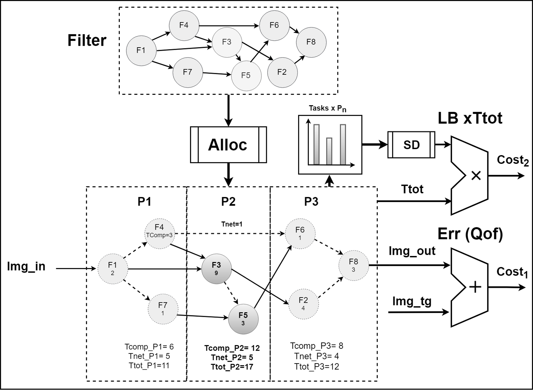Fn), each implementing one of the basic instructions, which are then mapped onto 3 processing nodes. The new filter is applied to img_in, and the resulting img_out is compared to the target image img_tg to determine $\textit{cost}_{1}$ . The computation time Ttot for the filter is determined by P2 (the solid arrows contribute to Tnet and the tasks F3 and F5 to the internal Tcomp). Ttot is then multiplied by the standard deviation SD of the processor loads, representing load balancing (LB) to compute $\textit{cost}_{2}$ . The two costs are then used in the multi-objective evolutionary process.

More complex operators, like opening and closing, among others, can be obtained by combining dilations and erosions algorithmically [35, 7]. These ideas can be extended to grey-level and colour image processing as well, using the maximum and minimum operators.

From these definitions, it can be evinced that the complexity (defined in terms of computational effort) of a MM filter has a strong dependence on the size of the structuring element $\bm{B}$ . A significant reduction in complexity can be achieved by decomposing the structuring elements into simpler components, at the cost however of loss of filter quality [9].

The first objective of the multi-objective algorithm presented in this paper (Fig. 1) will then be to decompose complex filters into simpler tasks (basic instructions) in such a way that the error introduced by the decomposition is minimised.

2.2 Many-core architectures

While numerous architectural variants have been proposed in the context of many-core systems research, the work presented in this article tries to preserve generality by limiting the assumptions made on the architecture:

•
The many-core system will consist of an arbitrary large number of processing nodes (experiments were run for 8, 16, and 32-node systems).
•
Each node has access to a “significant” amount of local memory (this, however, only impacts the size of the images that can be processed).
•
The nodes are connected by a deadlock-free Network-on-Chip (NoC) with a bandwidth sufficient to avoid congestion (again, largely a limit on image size).

Within this scenario, MM graphs (Fig. 1), can be considered as streaming applications [33, 34], where each node will receive images from upstream nodes, apply one or more MM operators, and then propagate the processed image to one or more downstream nodes, repeating this sequence operation for all images in the required set. It should be highlighted that this coarse-grained decomposition represents a departure from the vast majority of the literature that addresses MM implementations and is in fact complementary to, for example, FPGA- or GPU-based accelerators (in the sense that it does not preclude the presence of such accelerators within the many-core processing nodes).

In order for a graph of $\bm{T}$ MM tasks to be implemented on a many-core system consisting of $\bm{P}$ processing nodes (where generally but not necessarily $\bm{T}>\bm{P}$ ), tasks need to be grouped and allocated to individual nodes (Fig. 1). The quality of this mapping is fundamental for performance, in terms of computation time and resource utilization [36, 37, 38].

One component of the overall time required by each node to process each image is obviously the time (Tcomp) necessary for the computation of the MM tasks allocated to it. By removing backward dependencies, the use of streaming graphs reduces this to a linear sum of the time required for each task (which can be pre-computed, given the platform specifications).

In a realistic scenario, however, the time required for each node to receive and send data (particularly for large image sizes) cannot be ignored. Given a specific platform and a constant image size, a node’s Tnet is then a function of how many input and output images are sent or received by all the tasks mapped to it (as derived from the task graph).

In this streaming approach, the time Ttot required to process each image on $\bm{P}$ processors is then obviously bounded by the slowest processor in the pipeline:

$\displaystyle\textit{Ttot}=\textbf{Max}(\textit{Tcomp}_{i}+\textit{Tnet}_{i}:i% \in\bm{P})$ (4)

The performance of a mapping in terms of processing time is not the only measure of the quality of a mapping, since it provides no information as to how optimally the resources of the system are used. In terms of energy or in a multi-application scenario, for example, it becomes important to minimise the number of processors used to implement a filter and to equalise the computation across all nodes. In practice, this can be achieved by load balancing (LB) the computation across the processors or, in other words, by minimising the standard deviation of Ttot across all nodes.

Figure 2.
Block diagram for the iMMf-Ma architecture, and its 3 basic modules: training, testing, and mapping. The training module is used to evolve individuals (filters) according to two conflicting objectives. The Testing module is used to verify the performance of the solutions. The filter(s) selected by the user are mapped onto the many-core architecture in the mapping module.

The second objective of the multi-objective optimisation algorithm proposed in this article is to group and allocate (i.e. map) the filter tasks to processing nodes in such a way that the performance (in terms of computation time) and the use of resources (in terms of load balancing) are minimised.
2.3 Multi-objective optimisation

The quality of a filter implementation will thus depend on two metrics (Fig. 1), which correspond to the two objectives to be optimised. The $\textit{cost}_{1}$ metric (Quality of Filter or QoF) measures the ability of the filter to identify the desired features within an input image. To evaluate the $\textit{cost}_{2}$ metric (Quality of Mapping or QoM), the algorithm distributes the graph instructions among the processors, optimising Ttot and load balancing to reduce the total execution time.

In general, filters with high complexity (larger structuring elements and/or more instructions) will have the best visual quality, but will require more time for computation, implying a conflict between the two metrics.

Resolving this conflict implies defining the relative importance of the two objectives. This, however, depends on the requirements of the designer: an application that needs, for example, to meet real-time constraints would prioritise the QoM metric, whereas QoF might dominate in high-precision filters.

The algorithm described in this article targets the design-time optimisation of a given mathematical morphology application (using pattern detection as an example) on a many-core architecture with known architectural parameters (computation and communication speed, number of processing nodes, etc.). As in similar research (e.g. as in [39, 40]), a multi-objective evolutionary algorithm was used to find a Pareto front of mapping solutions, each representing a non-dominated trade-off between the two optimisation metrics, allowing the designer to select an implementation that matches application-specific requirements.

3. Mapping of morphological filters on many-core architectures (iMMf-Ma)

Figure 2 illustrates the general block diagram of the proposed iMMf-Ma system, which consists of three basic modules: training, testing and mapping.

3.1 Training module

The objective of the training module is to automatically generate, using a multi-objective algorithm [41, 42, 43, 44, 45] and training images, acyclic graphs (filters) constructed from a set of basic instructions.

The training module (Algorithm 3.1, Fig. 2) was implemented using the PlatEMO tool [46]. After initial tests with several MOEA algorithms (including NSGAII [47], NSGAIII [48], MOEAD [49], and SPEA2 [50]) revealed no statistically significant differences, NSGAII was selected. The standard algorithm was then modified to use a CGP-derived [51, 52] encoding that matched the problem with no crossover and with a point mutation that more accurately fits the encoding.

Table 1
Parameters and variables used in the algorithms

EA parameters	Description
N	Number of individuals (population size)
M	Dimension (number of objectives)
L	Number of genes in the chromosome
D	Number of alleles
MT_RT	Mutation rate
EVALUATION	Number of evaluations
App parameters	Description
N_PROC	Number of processors
MM_INSTR	Basic instructions
K_TRAIN	Number of images in the training set
K_TEST	Number of images in the test set
Variables	Description
chrm	Chromosome of one individual
pop	Population (set of chromosomes)
costs	$cost_{1},cost_{2}$
graphs	Graphs
k	Number of images in the current set
train_set	Set of training image pairs
test_set	Set of test image pairs
test	Test or training set selection
img_in	Set of input images
img_tg	Set of target images
img_out	Set of output images
cluster	Set of processors

For this module, the following parameters and inputs (Table 1) must be specified:

•

A set (train_set) containing pairs of training images (original + target), where the original is a binary or grey-scale image of any resolution and the target contains binary objects of interest present in its corresponding input;

•

A set (MM_INSTR) of morphological (dilation, erosion, etc.), arithmetic (addition, subtraction, etc.), and logic (and, or, not, etc.) basic instructions;

•

Parameters of operation of the modified NSGAII algorithm: N: population size; M: number of objectives of the multi-objective problem; L: chromosome length (number of genes); D: number of alleles in the chromosome; EVALUATION: number of generations; N_PROC: number of processors of the many-core architecture; MT_RT: mutation rate for the evolutionary strategy.

$pop\leftarrow\textbf{Initial\_Pop}(\textit{N, MM\_INSTR, D, N\_PROC})$

$aux\leftarrow 0$ Dodowhile

aux $\leqslant$ EVALUATION [costs] $\leftarrow$ Cost_Eval(pop, MM_INSTR, D, train_set, N_PROC) $[\textit{pop, pareto\_front}]\leftarrow\textbf{NSGAII}(\textit{pop, costs, N, % M, D, N\_PROC, MT\_RT})$ aux $++$

$[graphs]\leftarrow\textbf{GraphGen}(\textit{pareto\_front})$

return graphs, costs, pareto_front

iMMf-Ma Training

Figure 3.

Chromosome format: each gene identifies the MM instruction used, the graph nodes (up to two) that provide inputs for the instruction, and the processor to which the instruction is allocated within the many-core array. The genotype is coded as integers, which by means of the Decode_Chrm function are transformed into a program listing, containing instructions from Table 2, representing the current chromosome. The fourth argument of each gene (processor id) is used by the mapping module.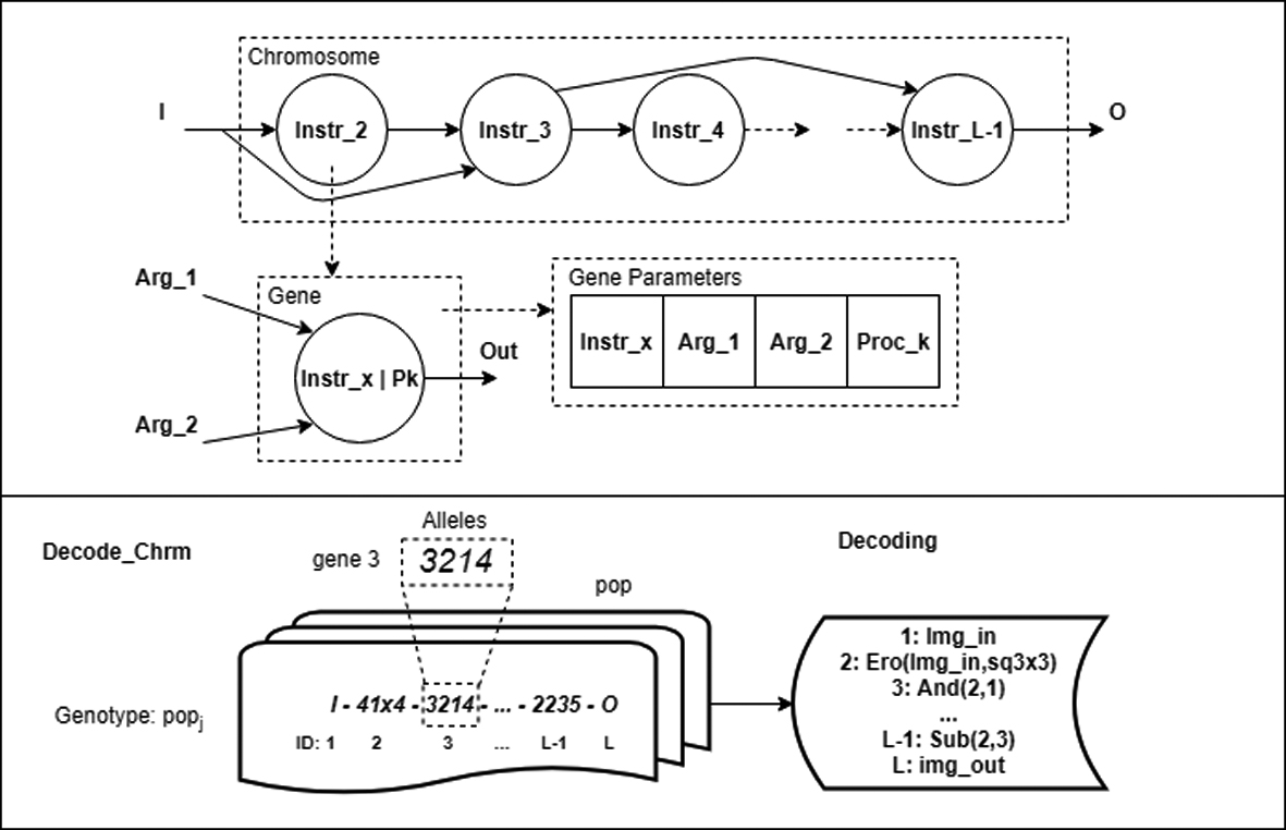

Given these, the algorithm outputs:

•

Pareto curves for the final population evolved, which can be used to select a filter satisfying user-specified requirements;

•

Application task graphs representing each individual, together with the associated filter parameters and processor allocations;

•

For visual verification purposes, the output images for the selected solution.

Table 2

MM basic instructions currently implemented in the iMMf-Ma system

ID	Instruction	Description	Complexity
1	Nop	No Operation. It allows a better flexibility for the chromosome, and of Arity 1.	1
2	Sub	Arithmetic Subtraction of Arity 2.	2
3	And	Logic And of Arity 2.	2
4	Ero_s_3	Erosion (Arity 2) by a square structuring element of size 3 $\times$ 3.	9
5	Ero_c_3	Erosion (Arity 2) by a disk shaped structuring element of size 3 $\times$ 3.	9
6	Ero_s_5	Erosion (Arity 2) by a square structuring element of size 5 $\times$ 5.	25
7	Ero_c_5	Erosion (Arity 2) by a disk shaped structuring element of size 5 $\times$ 5.	25
8	Ero_s_7	Erosion (Arity 2) by a square structuring element of size 7 $\times$ 7.	49
9	Ero_c_7	Erosion (Arity 2) by a disk shaped structuring element of size 7 $\times$ 7.	49
10	Dil_s_3	Dilation (Arity 2) by a square structuring element of size 3 $\times$ 3.	9
11	Dil_c_3	Dilation (Arity 2) by a disk shaped structuring element of size 3 $\times$ 3.	9
12	Dil_s_5	Dilation (Arity 2) by a square structuring element of size 5 $\times$ 5.	25
13	Dil_c_5	Dilation (Arity 2) by a disk shaped structuring element of size 5 $\times$ 5.	25
14	Dil_s_7	Dilation (Arity 2) by a square structuring element of size 7 $\times$ 7.	49
15	Dil_c_7	Dilation (Arity 2) by a disk shaped structuring element of size 7 $\times$ 7.	49
16	Ero_/_3	Erosion (Arity 2) by a right diagonal structuring element of size 3 $\times$ 3.	9
17	Ero__3	Erosion (Arity 2) by a left diagonal structuring element of size 3 $\times$ 3.	9
18	Ero_/_5	Erosion (Arity 2) by a right diagonal structuring element of size 5 $\times$ 5.	25
19	Ero__5	Erosion (Arity 2) by a left diagonal structuring element of size 5 $\times$ 5.	25
20	Ero_/_7	Erosion (Arity 2) by a right diagonal structuring element of size 7 $\times$ 7.	49
21	Ero__7	Erosion (Arity 2) by a left diagonal structuring element of size 7 $\times$ 7.	49
22	Dil_/_3	Dilation (Arity 2) by a right diagonal structuring element of size 3 $\times$ 3.	9
23	Dil__3	Dilation (Arity 2) by a left diagonal structuring element of size 3 $\times$ 3.	9
24	Dil_/_5	Dilation (Arity 2) by a right diagonal structuring element of size 5 $\times$ 5.	25
25	Dil__5	Dilation (Arity 2) by a left diagonal structuring element of size 5 $\times$ 5.	25
26	Dil_/_7	Dilation (Arity 2) by a right diagonal structuring element of size 7 $\times$ 7.	49
27	Dil__7	Dilation (Arity 2) by a left diagonal structuring element of size 7 $\times$ 7.	49
28	Or	Logic OR of Arity 2.	2
29	Nor	Logic NOR of Arity 2.	2
30	Add	Arithmetic Addition of Arity 2.	2

3.1.1 The evolutionary cycle

The training module relies on four main functions:

Initial_Pop: The initial population (pop) is generated randomly, based on the parameters N, MM_ INSTR, D and N_PROC. Each chromosome (Fig. 3) contains a set of genes that represent the nodes of the graph. Each gene consists of four alleles (although it is possible to use higher arity for its arguments if required): one instruction from an application specific set (Table 2), two input connections from previous nodes in the graph, and the id of the processor that will execute the instruction on the many-core architecture.

test $k\leftarrow\textbf{Size}(\textit{test\_set})$ $k\leftarrow\textbf{Size}(\textit{train\_set})$ $i\leftarrow 1$ $k$ test $\textit{img\_in}\leftarrow\textit{test\_set}_{i,1}$ ; $\textit{img\_tg}\leftarrow\textit{test\_set}_{i,2}$ $\textit{img\_in}\leftarrow\textit{train\_set}_{i,1}$ ; $\textit{img\_tg}\leftarrow\textit{train\_set}_{i,2}$ $j\leftarrow 1$ Size(pop) $\textit{chrm}_{j}\leftarrow\textbf{Decode\_Chrm}$ $(\textit{MM\_INSTR}_{pop_{j}},\textit{img\_in, D})$ $\textit{img\_out}_{i,j}\leftarrow\textbf{Eval}(chrm_{j})$ $\textit{costs}_{i,j,1}\leftarrow\textbf{Sum}(\textbf{Abs}(\textit{img\_out}_{i% ,j}-\textit{img\_tg}_{i,j}))/\textbf{Size}(\textit{img\_in})$ $\textit{Ttot}\leftarrow\textbf{Timing}(\textit{chrm}_{j},\textit{MM\_INSTR, D,% N\_PROC})$ $\textit{LB}\leftarrow\textbf{Std}(\textbf{Alloc}(\textit{chrm}_{j},\textit{N\_% PROC}))$ $\textit{costs}_{i,j,2}\leftarrow\textit{Ttot}*\textit{LB}$ return costsCost_Eval – computation of the metrics

Cost_Eval: This function (Algorithm 3.1.1) computes the metrics (see Section 2) for the current population pop. The metric formulae are detailed below in Section 3.1.2.

NSGAII: This function implements the NSGAII algorithms. Its inputs are the EA parameters, the current population pop and the metrics for each individual in the current population (costs). As output, the function returns the set of non-dominated individuals (pareto_front) among the filters in the current population (Fig. 4), together with the next generation to be evaluated (pop).

GraphGen: This function receives as input parameter the pareto_front generated by NSGAII, as mentioned above, and returns as output the corresponding graphs, which can be used to select the desired $\textit{cost}_{1}$ vs $\textit{cost}_{2}$ trade-off (Fig. 4).

3.1.2 Metrics

The metric evaluation is carried out as in Algorithm 3.1.1 through the application of a sequence of 5 functions: Decode_Chrm, Eval, Std, Alloc, and Timing.

Decode_Chrm, as its name suggests, decodes the chromosomes of the individuals in $\textit{pop}_{j}$ (genotype), of size ${D}$ , by means of a concatenation of instructions present in MM_INSTR, relative to their genes.

As an example, consider gene (graph_id: 3) of Fig. 3, with alleles “3-2-1-4”. From Table 2, the first allele 3 selects instruction AND, with the first input connected to the output of gene 2, and the second to img_in (gene 1). The instruction will be allocated to processor 4.

To evaluate the quality of the filters $\textit{chrom}_{j}$ generated by Decode_Chrm, the Eval function applies them to a set of training images and generates a set of corresponding output images ( $\textit{img\_out}_{i,j}$ ) (Fig. 3).

Figure 4.

Details of a point (Filter) of the Pareto curve generated by the NSGAII function. Costs has two columns, the first one referring to the filter error (Qof), and the second one to its complexity (total time through the pipeline (Tcomp 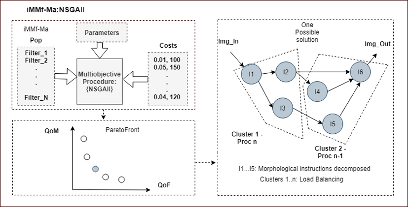$+$ Tnet) $\times$ SD of instructions distribution). Also, the clustering and allocation of instructions to processors to optimize the LB (Mapping Module) is shown. The graphs are generated by GraphGen.

The images in the $\textit{img\_out}_{i,j}$ set are then compared to the reference ones (img_tg), to produce the QoF metric $\textit{costs}_{i,j,1}$ . More specifically, this metric represents the Mean Absolute Error (MAE) between the images generated by applying each filter (graph) evolved by the tool and the target image for each image pair (original+target) in the training images set:

$\displaystyle\textit{MAE}=\frac{1}{XY}\sum_{i}^{X}\sum_{j}^{Y}|\textit{Iout}(i% ,j)-\textit{Itg}(i,j)|$ (5)

where Iout is the filtered image for one evolved filter, Itg is the target image corresponding to its img_in, and $({i},{j})$ is the pixel coordinate. ${X}$ and ${Y}$ are the dimensions of the image, used to average the error across all pixels.

By contrast, the evaluation of the QoM metric is much simpler, as it does not require the application to the filter to the image. As described in Section 2.2, given a specific target platform the processing time Tcomp for each node can be estimated by the linear sum of the complexities of each basic instruction (Table 2). The communication time Tnet can be derived from the task graph, as it corresponds to the number of input and output arcs of the tasks mapped to a specific processor (Fig. 1). This allows the algorithm, in the Timing function, to compute the first component (Ttot) of the QoM metric using Eq. (4) (it also evaluates the sequential execution time of the graph, for comparison purposes, as detailed in the Results section).

To evaluate the second component (LB) of the metric, which corresponds to load balancing, the algorithm computes the standard deviation of the processing time across all processors (Section 2.2). The two components are then multiplied together to direct the search towards more balanced individuals.

3.2 Testing module

The objective of the test module is to validate the graphs generated by the training module by applying a set of testing images.

For this, test_set, a new set of images, is used, containing different image pairs compared to the train_set training set. However, this new set contains the same image objects used in the training set, as it aims at validating the results generated from the training process. Thus, for the testing process, Algorithm 3.1.1 is also used to evaluate the metrics, and is applied to test_set rather than train_set. The graphs satisfying the requirements of the user are then passed to the mapping module to be allocated on the many-core architecture.

3.3 Mapping module

The objective of the mapping module is to cluster instructions (graph tasks) from the solution chosen by the user for implementation on the many-core architecture. This process would allow a platform-specific back-end to automatically generate the executables.

Figure 5.

Printed circuit board (PCB) image used for the experiments. The highlighted area shows the three types of patterns (square island, circle island, and track) to be extracted by the filter.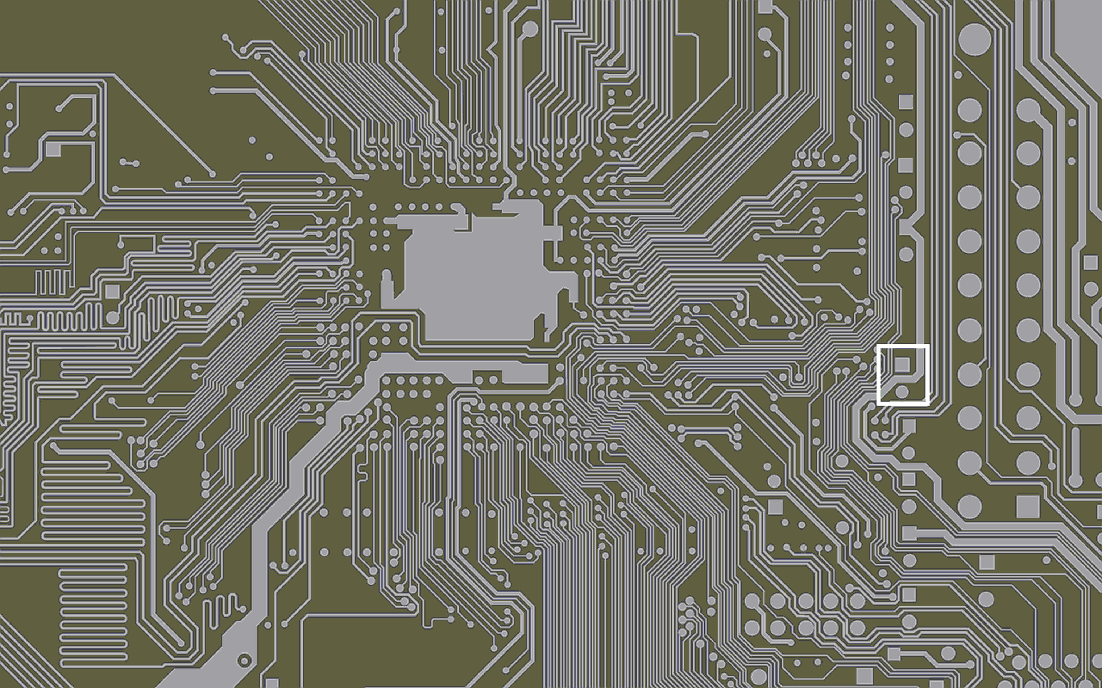

According to Fig. 3 (Section 3.1), the fourth allele of each gene (Proc_k), represents the processor to which the task will be allocated. Thus, the final objective of this module is to cluster the nodes of a given graph, generating an application mapping (Fig. 4). This process (Algorithm 3.3) receives the input parameters pop and L and returns the $\textit{cluster}_{aux,j-1}$ object, which corresponds to a set of processors of the many-core architecture containing allocated instructions from the application graph.

$i\leftarrow 1$ N_PROC $j\leftarrow 2$ $L-1$ $\textit{aux}\leftarrow\textit{chrm}_{j,4}$ $\textit{cluster}_{aux,j-1}\leftarrow j$

return cluster

Mapping module – clustering

Table 3

Experiment parameters

Parameters	Value
N	100
M	2
D	94
MT_RT	0.05
EVALUATION	10000
N_PROC	(8, 16, 32)
MM_INSTR	{1..15} from (Table 2)

Table 4

Mean and standard deviations of the filters evolved by the training module for each combination of pattern (circle island, square island and track), and numbers of processors (8, 16, and 32) over the 30 training samples. Three filters from each Pareto curve (the two extremes and one intermediate) were used in each case. Speedups are in bold in the table. As an example, the “Best Pareto” row represents, for each combination, the three points in the Pareto curve that contains the best QoF for an image pair

Processors/pattern	MAE	Ttot	Tseq	Speedup	MAE	Ttot	Tseq	Speedup	MAE	Ttot	Tseq	Speedup
	Best QoF				Intermediate				Best QoM
8/Circle Island
Avg	0.24	110.78	499.44	4.62	0.69	91.07	459.67	5.08	6.22	67.41	344.48	5.09
SD	0.24	27.55	99.24	0.79	0.60	16.26	85.13	0.71	3.79	16.90	96.94	0.60
Best Pareto	0.02	127.00	547.00	4.31	1.36	103.00	452.00	4.39	9.40	41.00	238.00	5.80
16/Circle Island
Avg	0.24	72.30	485.63	6.85	1.24	58.63	454.93	7.78	5.79	46.10	360.23	7.86
SD	0.18	15.73	92.49	1.14	1.84	12.20	103.07	1.11	2.75	10.82	93.71	1.08
Best Pareto	0.40	56.00	528.00	9.43	0.70	61.00	498.00	8.16	5.98	53.00	448.00	8.45
32/Circle Island
Avg	0.41	63.37	522.10	8.59	1.71	49.66	485.07	9.74	5.33	39.10	392.80	10.07
SD	0.34	16.82	85.98	1.93	1.98	7.12	110.03	1.63	3.14	12.12	143.11	1.92
Best Pareto	0.40	61.00	561.00	9.20	1.00	51.00	529.00	10.37	3.94	51.00	554.00	10.86
8/Square Island
Avg	7.36	121.33	528.87	4.49	7.74	96.37	482.73	5.03	9.37	89.00	468.07	5.35
SD	10.37	29.32	91.13	0.83	9.58	16.00	84.70	0.51	7.20	17.72	66.71	0.70
Best Pareto	0.02	101.00	408.00	4.04	0.09	72.00	370.00	5.14	1.51	65.00	425.00	6.54
16/Square Island
Avg	7.33	91.57	559.03	6.39	7.62	64.90	505.07	7.89	9.92	58.90	467.00	7.96
SD	10.39	22.55	64.98	1.41	9.85	9.34	56.82	1.12	7.40	8.43	83.40	1.13
Best Pareto	0.03	101.00	567.00	5.61	1.87	61.00	495.00	8.11	6.89	61.00	545.00	8.93
32/Square Island
Avg	7.33	68.87	543.90	8.18	7.85	52.77	511.57	9.69	8.84	48.43	480.60	9.81
SD	10.37	15.51	64.29	1.65	10.17	2.73	102.06	1.87	6.53	7.91	121.45	1.50
Best Pareto	0.27	52.00	519.00	9.98	0.57	51.00	551.00	10.80	5.49	52.00	595.00	11.44
8/Track
Avg	4.31	80.85	387.54	4.85	5.72	75.23	393.38	5.21	8.62	65.46	314.62	4.88
SD	4.53	17.14	91.88	0.83	4.92	15.78	97.97	0.60	11.37	21.21	91.50	0.65
Best Pareto	0.08	57.00	307.00	5.39	0.45	63.00	293.00	4.65	1.29	47.00	253.00	5.38
16/Track
Avg	2.91	67.47	412.63	6.27	2.93	56.20	378.80	6.83	4.87	46.50	337.63	7.30
SD	3.94	67.47	112.58	1.20	3.18	18.45	117.77	1.06	7.99	15.98	126.66	1.27
Best Pareto	0.08	55.00	316.00	5.75	0.86	51.00	292.00	5.73	1.29	37.00	266.00	7.19
32/Track
Avg	2.68	58.36	441.64	8.00	2.75	47.07	397.54	8.72	3.56	42.75	411.29	9.76
SD	3.72	19.67	100.31	1.84	3.16	13.42	102.97	1.73	3.60	11.12	116.23	1.91
Best Pareto	0.45	27.00	338.00	12.52	0.48	27.00	307.00	11.37	2.12	27.00	424.00	15.70

4. Experimental results

The lack of literature addressing the issue of mapping MM applications on many-core systems prevents a comparative evaluation of the tools. Performance comparisons with FPGA-based hardware accelerators (e.g. [19, 20, 21, 18]), besides being unrealistic as the images used for benchmarking in the literature are generally much smaller than the one used for the experiments in this paper, would also be largely irrelevant, since the two approaches are entirely compatible. In fact, should the many-core system nodes allow the implementation of hardware accelerators, this feature could be integrated in the proposed tool to improve Tcomp and thus shift the Pareto curve.

The results proposed in this article thus rely on implicit benchmarking: in order to evaluate the performance ( $\textit{cost}_{1}$ ) of the iMMf-Ma approach, the algorithm was applied to a real world application aimed at recognising patterns in printed circuit boards (PCB) images, which could be used to detect imperfections.

Figure 6.

Example of an iMMf-Ma system result for square island detection in an 8-processor pipeline. Each point represents a chromosome (generated filter) in the final population. The green line connects non-dominated solutions on the Pareto curve.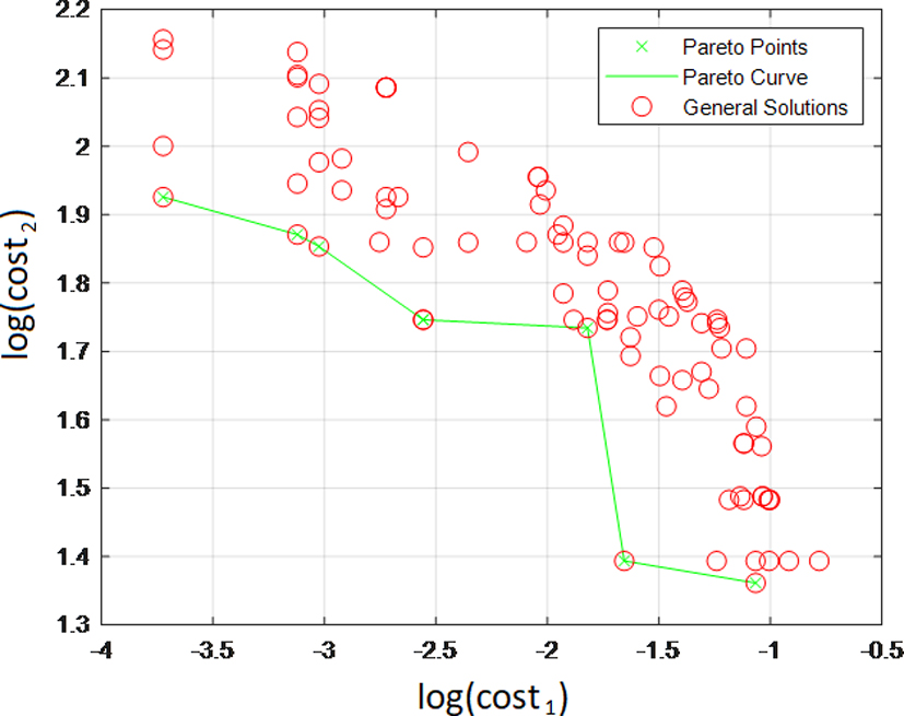

Table 5

Mean, standard deviations and selected individual (bold) obtained from the testing process for the Best QoF filters

Processors/pattern		Test_Image_1 (MAE)	Test_Image_2 (MAE)	Test_Image_2 (MAE)
8/Circle Island	Avg	2.96	5.15	3.20
	SD	1.23	2.51	1.26
	Best MAE	0.12	0.15	0.68
	Best MAE SD	0.04	0.06	0.25
16/Circle Island	Avg	3.91	4.93	6.33
	SD	1.61	1.48	2.00
	Best MAE	0.08	0.37	0.94
	Best MAE SD	0.02	0.12	0.32
32/Circle Island	Avg	4.28	5.32	5.02
	SD	1.76	2.00	1.57
	Best MAE	0.07	10.46	2.72
	Best MAE SD	0.02	3.03	0.96
8/Square Island	Avg	0.59	0.93	3.42
	SD	0.87	0.76	1.31
	Best MAE	0.02	0.06	0.96
	Best MAE SD	0.01	0.02	0.29
16/Square Island	Avg	2.97	1.68	4.38
	SD	2.58	1.00	1.97
	Best MAE	0.02	0.06	1.24
	Best MAE SD	0.01	0.02	0.86
32/Square Island	Avg	3.06	1.69	4.35
	SD	2.19	0.77	2.03
	Best MAE	0.06	0.40	1.39
	Best MAE SD	0.02	0.16	0.60
8/Track	Avg	5.64	5.58	9.03
	SD	2.95	2.63	3.69
	Best MAE	4.70	0.51	1.43
	Best MAE SD	1.81	0.16	0.16
16/Track	Avg	6.31	6.76	10.81
	SD	3.90	3.05	4.79
	Best MAE	0.63	0.24	5.43
	Best MAE SD	0.54	0.20	1.58
32/Track	Avg	7.37	5.44	7.13
	SD	3.87	2.37	2.86
	Best MAE	0.49	5.61	11.27
	Best MAE SD	0.38	1.43	4.82

The train_set and test_set sets (Section 3.1) use binary sub-images from the original monochrome image of Fig. 5, with a spatial resolution of 3277 $\times$ 2048 pixels. The objective was to detect 3 types of patterns:circle islands, square islands, and tracks, of sizes defined by the highlighted region (rectangle) in the figure.

The EA parameters used in the experiments are described in Table 3 (the parameter values were derived through a set of calibration experiments). To evaluate the scalability of the algorithms, three different sizes of many-core architectures were used in the training and testing processes: 8, 16, and 32 processors. For the current application, only instructions 1 to 15 in Table 2 were necessary, due to the geometry of the objects to be detected. Because of the nature of the problem, a limit of two inputs per node was imposed on the graph, a restriction that can be relaxed by a tool parameter.

All time metrics were computed as a function of complexity, which is proportional to the number of active pixels in the structuring elements used by the morphological operations. Thus, for the morphological operations, the convention adopted was to consider the dimensions of the structuring elements to determine Tcomp for each base operation (Table 2). The complexities of the other operations were derived through comparison to the morphological operations.

Figure 7.

Visual results obtained for the circle island testing process for 8 processors and 2 different points of the Pareto curve.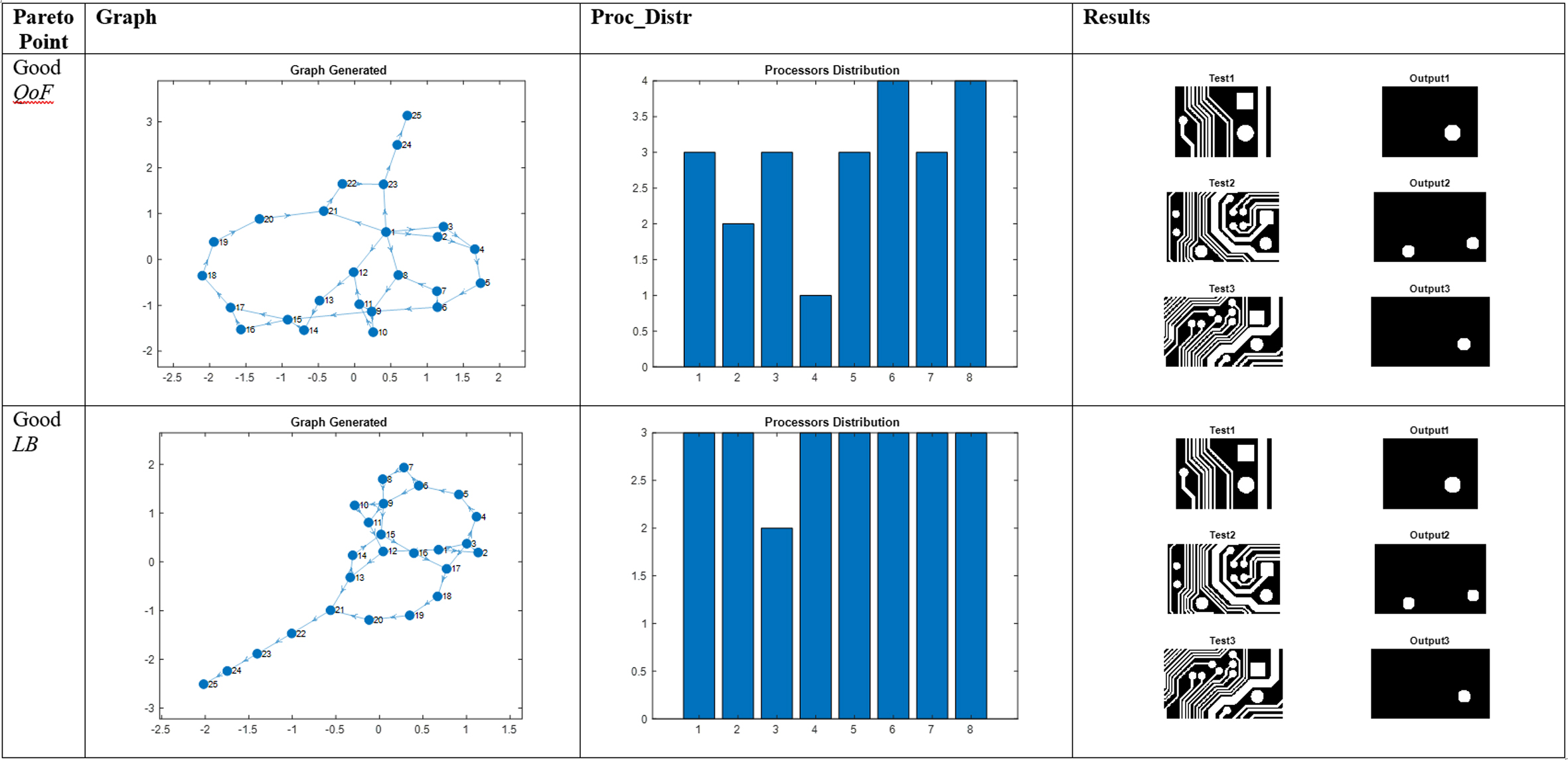

Figure 8.

Visual results obtained for the square island testing process for 8 processors and 2 different points of the Pareto curve.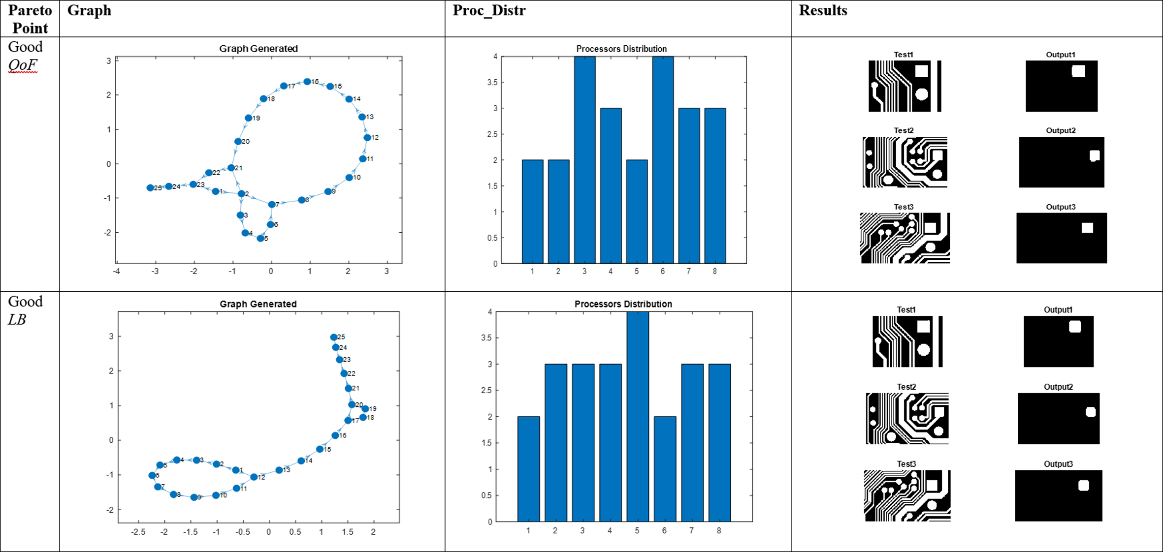

Figure 9.

Visual results obtained for the Track Testing Process for 8 processors and 2 different points of the Pareto curve.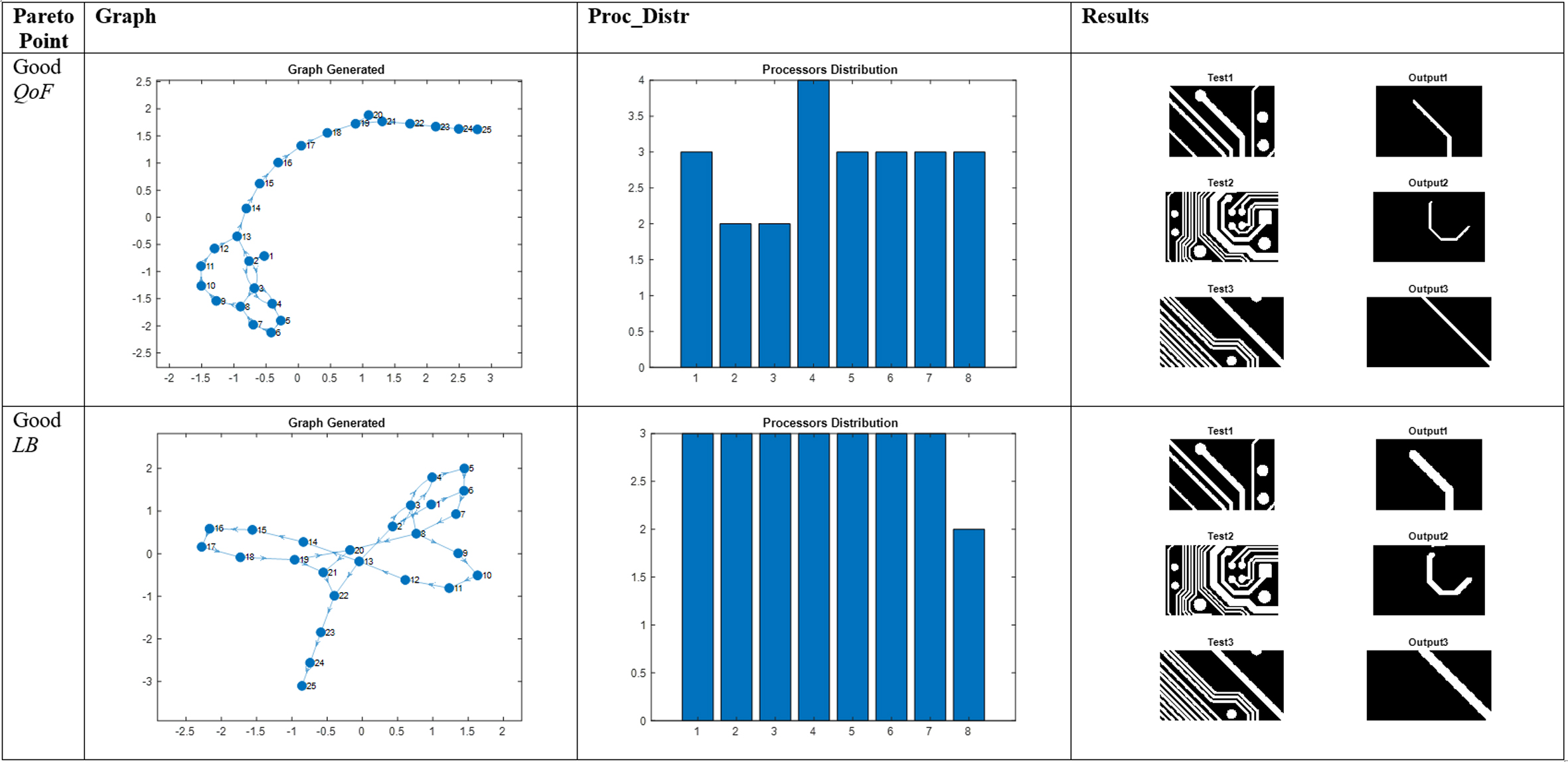

Given the assumptions on the NoC capabilities (Section 2.2) and the features of the application, Tnet was set to a constant value of 1 for each arc in the graph. It is important to note that, for the purposes of the EA, the units used in the estimation of the computational complexity are irrelevant, as long as the ratio between the component values matches their execution time in the target platform. Non-exhaustive empirical tests performed on a single-processor machine confirmed that the timing relationship between the instructions closely matches the complexity-based estimations.

4.1 Experiments

For the training process, 30 pairs of sample images (130 $\times$ 122 pixels) were used, cut out at random positions from Fig. 5, each containing the three types of patterns mentioned above and for the three many-core system sizes (for a total of 270 training examples). All the images were binarized prior to this process.

The output of the training process is a set of Pareto curves that present the non-dominated solutions obtained for each image pair. Figure 6 shows an example of a curve generated by the tool, for an architecture containing 8 processors with square island detection.

The results obtained in the training phase are summarized in Table 4. For each configuration (number of processors and pattern combination), three individuals (filters) were selected from the Pareto fronts of each image pair: best QoF, best QoM, and an intermediate solution. The table then displays the average and standard deviation of the MAE and Ttot across all individuals (note that the total execution time Ttot was selected over $\textit{cost}_{2}$ as being clearer and more relevant in a design context).

To provide a comparison metric, the table also includes averages and SDs for Tseq, the execution time of each individual on a single processor (computed by setting Tnet to 0 and adding together the execution times of each instruction in the chromosome). This parameter then allows the calculation of the speedup (SeqT/Ttot) obtained through the parallelisation of the filter. The analysis of the values in Table 4 reveals that, as expected, the speedup in all cases is increasing with the number of processors.

Selected individuals among those found by the training process are then input to the testing process, where their performance is evaluated on the set of test images.

In a user scenario, the selection of individuals to be tested would be guided by the design priorities. For example, if the application requires a high-quality filter (low MAE) and performance (Ttot) is not a constraint, the “best QoF” column of Table 4 would be used to select individuals to be tested. In a real-time system that needs to minimise processing time, even if this implies lower visual quality for the filter (high MAE), tests would focus on individuals from the “best QoM” column. In cases where the two constraints have the same weight, the intermediate individuals provide a viable solution. Of course, the designer would be able to pick any of the Pareto points in the graph depending on requirements and not be limited to the three that were arbitrarily selected for Table 4.

For this article, in order to carry out a more thorough evaluation of the performance of the approach, three individuals (best QoF, best QoM, and an intermediate result) from each image pair (for a total of 270 chromosomes) were selected for testing.

Each filter was applied to three different test image pairs of 248 $\times$ 183, 344 $\times$ 216, and 356 $\times$ 211 pixels, respectively, cut out at random positions in Fig. 5, for a total of 810 tests.

Table 5 shows an example of the results obtained for the set of best QoF individuals. For each combination of processors and patterns, the first two lines of the table refer to the MAE of all filters on each test image.

The third and fourth lines represent an individual selected from all the tested candidates as providing the best visual results. As other works in the literature have highlighted [12, 10], considering only the MAE in an image processing context is not the best option. The choice thus corresponds to solutions with the smallest SD, a more useful metric for visual quality.

The results were additionally verified through visual inspection (see examples in Figs 7–9). In every case, two individuals were selected for the tests: the first with low standard deviation (lower MAE) and the second with better speedup (lower Ttot and better load balancing (LB)). For example, in Fig. 9 (track detection), the tracks found by the second filter are marginally thicker than the first (higher MAE) but the mapping displays significantly better Ttot and load balancing (LB – visualised in the histograms).

5. Conclusions

Many-core architectures, while still at an embryonic stage of development, seem to represent ideal platforms for the implementation of mathematical morphology applications: as systolic, distributed-memory arrays of processing cores, they are well suited to handle the high computational demands of MM, particularly when the latter is decomposed into simpler operations, allowing the system to exploit instruction streaming.

In this paper, a typical MM application (a filter for pattern detection) was used to explore the use of multi-objective optimisation of many-core implementations. The MO algorithm is able to find a range of different non-dominated mappings that represent optimal trade-offs between the visual quality of the filter and computational performance on a many-core system. In this work, the assumptions made with respect to the many-core architecture are kept to a minimum to preserve the generality of the solutions. Within this scenario, the algorithm attempts to model realistic constraints by taking into account not only computation time, but also the time required for data transfers and the efficient use of resources by balancing the load across processors.

The approach was evaluated using a pattern recognition filter applied to a high-quality (3277 $\times$ 2048 pixels) PCB image. The tools proved capable of providing a set of solutions for 8, 16, and 32 core systems, taking into account both computation and communication time in the array, where each solution represents a mapping of MM instructions to cores. Rather than arbitrarily selecting a quality/performance trade-off, the approach presented in this paper outputs a Pareto curve of solutions representing a range of trade-off points. Aimed to a design tool for MM applications, it leaves the choice of the most appropriate compromise to the designer: by a simple selection of the desired performance and/or quality targets, the designer is able to select a mapping that meets specifications and can be implemented in the target many-core system.

Footnotes

Acknowledgments

The first author is grateful to FAPESP (Grant 2017/ 26421-3) and CAPES. This work was partially supported through the EPSRC Graceful Project (Grant EP/ L000563/1).

References

Dougherty

Astola

. An introduction to nonlinear image processing. vol. 16. SPIE Press. 1994.

Serra

. Image analysis and mathematical morphology. Academic Press, Inc. 1983.

Soille

. Morphological image analysis: Principles and applications. Springer Science & Business Media. 2013.

Sonka

Hlavac

Boyle

. Image processing, analysis, and machine vision. Cengage Learning. 2014.

Maragos

. Lattice image processing: A unification of morphological and fuzzy algebraic systems. Journal of Mathematical Imaging and Vision. 2005; 22(2-3): 333-353.

Ortiz

Torres

De Juan

Cuenca

. Colour mathematical morphology for neural image analysis. Real-Time Imaging. 2002; 8(6): 455-465.

Gonzalez

Wintz

. Digital image processing. Addison-Wesley Publishing Co. (Applied Mathematics and Computation). 1977.

Angulo

Serra

. Morphological coding of color images by vector connected filters. in: Proc. 7th Int. Symp. on Signal Processing and its Applications. Vol. 1. IEEE. 2003; 69-72.

Pedrino

Saito

Roda

. A genetic programming approach to reconfigure a morphological image processing architecture. International Journal of Reconfigurable Computing. 2011; 2011: 5.

10.

Yoda

Yamamoto

Yamada

. Automatic acquisition of hierarchical mathematical morphology procedures by genetic algorithms. Image and Vision Computing. 1999; 17(10): 749-760.

11.

Pedrino

Roda

Kato

ERR

Saito

Tronco

Tsunaki

, et al. A genetic programming based system for the automatic construction of image filters. Integrated Computer-Aided Engineering. 2013; 20(3): 275-287.

12.

Quintana

Poli

Claridge

. Morphological algorithm design for binary images using genetic programming. Genetic Programming and Evolvable Machines. 2006; 7(1): 81-102.

13.

Zhao

Guo

Zhou

Zhang

. A quantum-inspired genetic algorithm-based optimization method for mobile impact test data integration. Computer-Aided Civil and Infrastructure Engineering. 2018; 33(5): 411-422.

14.

Valenzuela

Jiang

Carrillo

Rojas

. Multi-objective genetic algorithms to find most relevant volumes of the brain related to alzheimer’s disease and mild cognitive impairment. International Journal of Neural Systems. 2018; 28(9): 1850022.

15.

Haralick

Sternberg

Zhuang

. Image analysis using mathematical morphology. IEEE Transactions on Pattern Analysis and Machine Intelligence. 1987; PAMI-9(4): 532-550.

16.

Bartovsky

Dokladalova

Dokládal

Georgiev

. Pipeline architecture for compound morphological operators. in: 2010 IEEE International Conference on Image Processing. IEEE. 2010; 3765-3768.

17.

Pedrino

Roda

. Real-time morphological pipeline architecture using high-capacity programmable logical devices. Journal of Electronic Imaging. 2007; 16(2): 023002.

18.

Elloumi

Krid

Sellami

. 2D parallel architecture for morphological operators supporting multiple shaped structuring elements. Procedia Computer Science. 2018; 126: 695-702.

19.

Gibson

Ahmadinia

McMeekin

Strang

Morison

. A reconfigurable real-time morphological system for augmented vision. EURASIP Journal on Advances in Signal Processing. 2013; 2013(1): 134.

20.

Holzer

Schumacher

Greiner

Rosenstiel

. Optimized hardware architecture of a smart camera with novel cyclic image line storage structures for morphological raster scan image processing. in: 2012 IEEE International Conference on Emerging Signal Processing Applications. IEEE. 2012; 83-86.

21.

Mukherjee

Mukhopadhyay

Biswas

. FPGA based parallel implementation of morphological filters. in: 2016 International Conference on Microelectronics, Computing and Communications (MicroCom). IEEE. 2016; 1-6.

22.

Chien

Chen

. Partial-result-reuse architecture and its design technique for morphological operations with flat structuring elements. IEEE Transactions on Circuits and Systems for Video Technology. 2005; 15(9): 1156-1169.

23.

Hedberg

Kristensen

Owall

. Low-complexity binary morphology architectures with flat rectangular structuring elements. IEEE Transactions on Circuits and Systems I: Regular Papers. 2008; 55(8): 2216-2225.

24.

Thurley

Danell

. Fast morphological image processing open-source extensions for GPU Processing with CUDA. IEEE Journal of Selected Topics in Signal Processing. 2012 Nov; 6(7): 849-855.

25.

Karas

Morard

Bartovsky

Grandpierre

Dokladalova

Matula

, et al. GPU implementation of linear morphological openings with arbitrary angle. Journal of Real-Time Image Processing. 2012; 04; 10.

26.

Youkana

Cousty

Saouli

Akil

. Parallelization strategy for elementary morphological operators on graphs: Distance-based algorithms and implementation on multicore shared-memory architecture. Journal of Mathematical Imaging and Vision. 2017; 59(1): 136-160.

27.

Valencia

Plaza

. Efficient implementation of morphological opening and closing by reconstruction on multi-core parallel systems. in: 2009 First Workshop on Hyperspectral Image and Signal Processing: Evolution in Remote Sensing. IEEE. 2009; 1-4.

28.

Vajda

. Programming many-core chips. Springer Verlag. 2011.

29.

Adeli

. Parallel processing in computational mechanics. New York, NY, USA: Marcel Dekker. 1992.

30.

Adeli

Hung

. A concurrent adaptive conjugate gradient learning algorithm on MIMD shared-memory machines. The International Journal of Supercomputing Applications. 1993; 7(2): 155-166.

31.

Hung

Adeli

. Parallel backpropagation learning algorithms on Cray Y-MP8/864 supercomputer. Neurocomputing. 1993; 5(6): 287-302.

32.

Adeli

Kumar

. Concurrent structural optimization on massively parallel supercomputer. Journal of Structural Engineering. 1995; 121(11): 1588-1597.

33.

Gordon

Thies

Amarasinghe

. Exploiting coarse-grained task, data, and pipeline parallelism in stream programs. SIGPLAN Not. 2006 Oct; 41(11): 151-162. Available from: http://acm.org/10.1145/1168918.1168877.

34.

Holzenspies

PKF

Hurink

Kuper

Smit

GJM

. Run-time spatial mapping of streaming applications to a heterogeneous multi-processor system-on-chip (MPSOC). in: 2008 Design, Automation and Test in Europe. 2008; 212-217.

35.

Dougherty

Lotufo

. Hands-on morphological image processing. vol. 59. SPIE Press. 2003.

36.

Radu

Mahbub

VinÅ£an

. Developing domain-knowledge evolutionary algorithms for network-on-chip application mapping. Microprocessors and Microsystems. 2013; 37(1): 65-78. Available from: https://www-sciencedirect-com.web.bisu.edu.cn/science/article/pii/S0141933112001901.

37.

Sahu

Chattopadhyay

. A survey on application mapping strategies for Network-on-Chip design. Journal of Systems Architecture. 2013; 59(1): 60-76. Available from: https://www-sciencedirect-com.web.bisu.edu.cn/science/article/pii/S1383762112000902.

38.

Singh

Shafique

Kumar

Henkel

. Mapping on multi/many-core systems: Survey of current and emerging trends. in: 2013 50th ACM/EDAC/IEEE Design Automation Conference (DAC). 2013; 1-10.

39.

Rostami

Neri

. Covariance matrix adaptation pareto archived evolution strategy with hypervolume-sorted adaptive grid algorithm. Integrated Computer-Aided Engineering. 2016; 23(4): 313-329.

40.

Rostami

Neri

Epitropakis

. Progressive preference articulation for decision making in multi-objective optimisation problems. Integrated Computer-Aided Engineering. 2017; 24(4): 315-335.

41.

Gutierrez Soto

Adeli

. Many-objective control optimization of high-rise building structures using replicator dynamics and neural dynamics model. Structural and Multidisciplinary Optimization. 2017; 56(6): 1521-1537.

42.

Shen

. Shape generation of grid structures by inverse hanging method coupled with multiobjective optimization. Computer-Aided Civil and Infrastructure Engineering. 2018; 33(6): 498-509.

43.

Wang

Szeto

. Multiobjective environmentally sustainable road network design using pareto optimization. Computer-Aided Civil and Infrastructure Engineering. 2017; 32(11): 964-987.

44.

Wang

Zukerman

Guo

Wang

, et al. Multiobjective path optimization for critical infrastructure links with consideration to seismic resilience. Computer-Aided Civil and Infrastructure Engineering. 2017; 32(10): 836-855.

45.

Taillandier

Fernandez

Ndiaye

. Real estate property maintenance optimization based on multiobjective multidimensional knapsack problem. Computer-Aided Civil and Infrastructure Engineering. 2017; 32(3): 227-251.

46.

Tian

Cheng

Zhang

Jin

. PlatEMO: A MATLAB platform for evolutionary multi-objective optimization. IEEE Computational Intelligence Magazine. 2017; 12(4): 73-87.

47.

Deb

Agrawal

Pratap

Meyarivan

. A fast elitist non-dominated sorting genetic algorithm for multi-objective optimization: NSGA-II. in: International Conference on Parallel Problem Solving From Nature. Springer. 2000; 849-858.

48.

Deb

Jain

. An evolutionary many-objective optimization algorithm using reference-point-based nondominated sorting approach, part i: Solving problems with box constraints. IEEE Transactions on Evolutionary Computation. 2013; 18(4): 577-601.

49.

Zhang

. MOEA/D: A multiobjective evolutionary algorithm based on decomposition. IEEE Transactions on Evolutionary Computation. 2007; 11(6): 712-731.

50.

Zitzler

Laumanns

Thiele

. SPEA2: Improving the strength Pareto evolutionary algorithm. TIK-report. 2001; 103.

51.

Koza

. Genetic programming: On the programming of computers by means of natural selection. Cambridge, MA, USA: MIT Press. 1992.

52.

Miller

Thomson

Fogarty

. Designing electronic circuits using evolutionary algorithms. Arithmetic Circuits: A Case Study. Wiley. 1997.

A multiobjective metaheuristic approach for morphological filters on many-core architectures

Abstract

Keywords

1. Introduction

2. Fundamentals

2.1 Mathematical morphology

3. Mapping of morphological filters on many-core architectures (iMMf-Ma)

3.1 Training module

Table 1 Parameters and variables used in the algorithms

3.1.2 Metrics

3.3 Mapping module

5. Conclusions

Footnotes

Acknowledgments

References

Table 1
Parameters and variables used in the algorithms