Algorithm for placement of reference points and choice of an appropriate variable shape parameter for the RBF approximation

Abstract

Many Radial Basis Functions (RBFs) contain a shape parameter which has an important role to ensure good quality of the RBF approximation. Determination of the optimal shape parameter is a difficult problem. In the majority of papers dealing with the RBF approximation, the shape parameter is set up experimentally or using some ad-hoc method. Moreover, the constant shape parameter is almost always used for the RBF approximation, but the variable shape parameter produces more accurate results. Several variable shape parameter methods, which are based on random strategy or on an evolutionary algorithm, have been developed. Another aspect which has an influence on the quality of the RBF approximation is the placement of reference points.

A novel algorithm for finding an appropriate set of reference points and a variable shape parameter selection for the RBF approximation of functions $y=f(x)$ (i.e. the case when a one-dimensional dataset is given and each point from this dataset is associated with a scalar value) is presented. Our approach has two steps and is based on exploiting features of the given dataset, such as extreme points or inflection points, and on comparison of the first curvature of a curve. The proposed algorithm can be used for the approximation of data describing a curve parameterized by one variable in multidimensional space, e.g. a robot path planning, etc.

Keywords

Radial basis functions approximation variable shape parameter curvature Lagrange multipliers

1. Introduction

Radial basis functions (RBFs) are used to solve many technical and non-technical problems. RBFs are real-valued functions which depend only on the distance from the fixed center point. A RBF method was originally introduced by [1, 2]. It is a powerful tool for the meshless interpolation and approximation of scattered data, as space tessellation is not required. Moreover, this method is independent with respect to the dimension of the space. RBF applications can be found in data visualization [3], surface reconstruction [4, 5, 6], vector fields visualization [7], solving partial differential equations [8, 9], etc.

RBFs can be divided into two main groups of basis functions: global RBFs and Compactly Supported RBFs (CS-RBFs) [10]. The use of CS-RBFs leads to a simpler and faster computation, because a system of linear equations has a sparse matrix. However, approximation using CS-RBFs is quite sensitive to the density of given scattered data. Global RBFs are useful in repairing incomplete datasets and they are significantly less sensitive to the density of data as they cover the whole domain. However, they lead to a linear system of equations with a dense and ill-conditioned matrix.

Choice of an appropriate shape parameter of RBFs is extremely important to ensure good approximation. Several articles have been dedicated to introducing different algorithms to compute a constant value as an appropriate value for the shape parameter [11, 12, 13, 14], etc. Many of these focus on finding the minimal error in computations or are based on convergence analysis. Other articles show that variable shape parameters are useful instead of a fixed shape parameter. Sufficient conditions to guarantee a unique solution of the RBF interpolation with variable shape parameters are derived in [15] for CS-RBFs and in [16] for global RBFs. The variable shape parameters are determined by used of genetic algorithm [17] and minimization of the local cost function [18, 19] or numerically by minimizing the root-mean-square errors [20]. For these purposes, there are many other papers which are dealing with the general global optimization such as [21, 22, 23]. Other approaches generate the variable shape parameters from an estimated range when different distributions of values are used [24, 25], use Neural Network RBF approach [26, 27, 28, 29, 30] or orthogonal least square [31]. However, the approaches mentioned do not reflect features of the given data.

Our approach for 1.5D case eliminating above mentioned drawbacks will be described in this paper. The proposed method consists of two steps. In the first step, the Thin-Plate Spline (TPS) function is used. The second step is focused on RBFs which have smoothness at least $C^{3}$ at the origin (e.g. Gaussian RBF, Wendland’s $\phi_{3,2}$ , etc.). This condition follows from the requirement that the first curvature of curves is smooth, which is a direct result of the algorithm described below. The proposed approach leads to a significant compression of the given data and obtaining their analytical form. Our approach can be applied to many real data in the different areas of interest, e.g. data obtained from GPS navigation describing the terrain profile [32], data for recovering smooth robot trajectory [33], total electron content data [34], etc.

In the following section, the fundamental theoretical background needed for description of the proposed algorithm will be mentioned. The proposed two steps algorithm, including the derivation of the appropriate variable shape parameter, will be described in Section 3. The results of the proposed algorithm for synthetic and real data will be presented in Section 4.

2. Theoretical background

In this section, some theoretical aspects needed for description of the proposed algorithm for placement of reference points and choice of an appropriate variable shape parameter for the RBF approximation will be introduced.

2.1 RBF approximation with a variable shape parameter

We assume that we have an unordered dataset $\{\bm{x}_{i}\}_{1}^{N}\in\mathbb{E}^{n}$ , where $n$ denotes the dimension of space. Further, each point $\bm{x}_{i}$ from the dataset is associated with a vector $\bm{h}_{i}\in\mathbb{E}^{p}$ of the given values, where $p$ is the dimension of the vector, or a scalar value, i.e. $h_{i}\in\mathbb{E}^{1}$ . In the following, we will deal with scalar data approximation, i.e. the case when each point $\bm{x}_{i}$ is associated with a scalar value $h_{i}$ is considered. Let us introduce a set of new reference points (knots of RBF) $\{\bm{\xi}_{j}\}_{1}^{M}\in\mathbb{E}^{n}$ , where $n$ denotes the dimension of space, $M$ is the number of reference points and $M\ll N$ .

These reference points may not necessarily have any special distribution as uniform distribution, etc. However, a good placement of the reference points improves the approximation of the underlying data. The RBF approximation is based on the distance computation between the given point $\bm{x}_{i}$ and the reference point $\bm{\xi}_{j}$ .

Figure 1.

RBF collocation functions centered at reference points $\{\bm{\xi}_{j}\}\in\mathbb{E}^{2}$ .

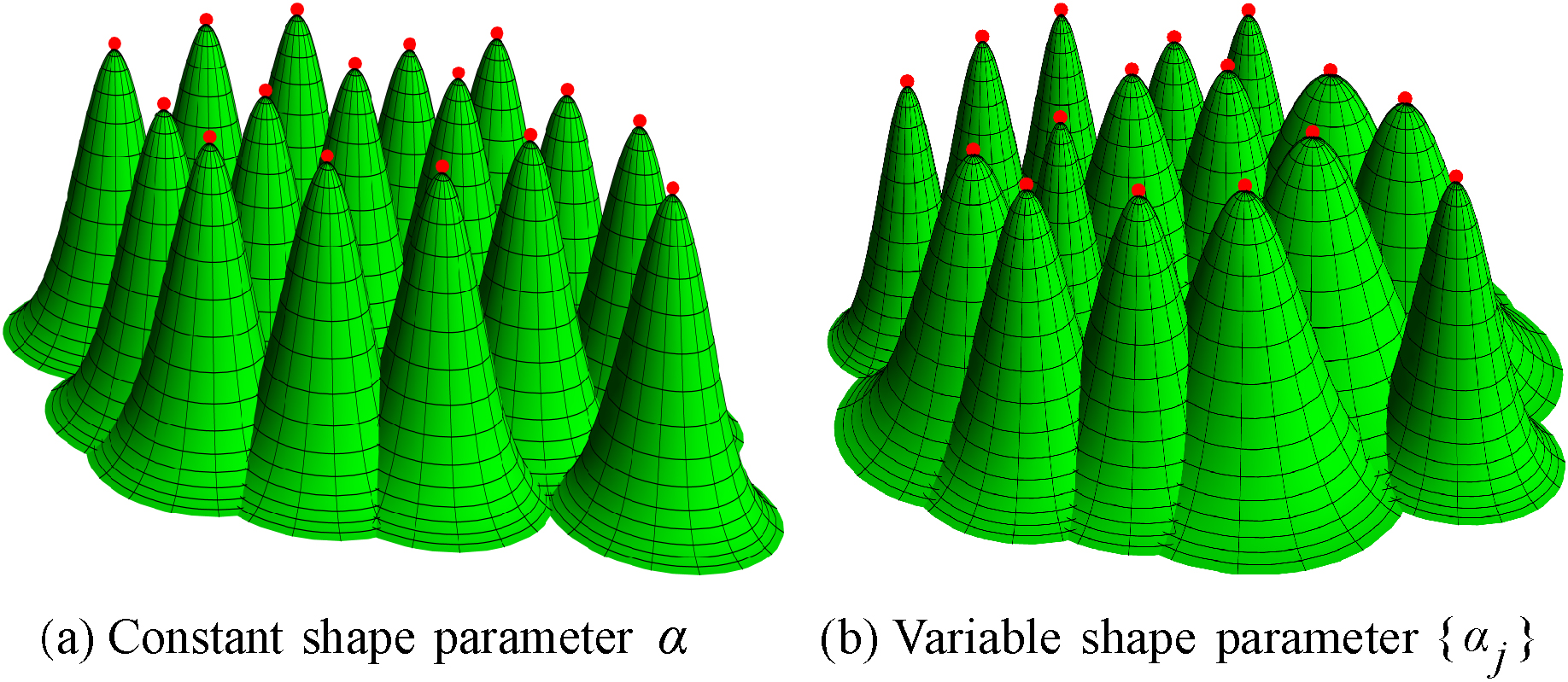
As generally known, most RBFs are dependent on the shape parameter $\alpha$ , which influences the radius of support. In the case of the fundamental RBF approximation (see [35, 36, 37]), the shape parameter of the RBF used is set to a constant value for all $M$ RBFs, see Fig. 1a. Nevertheless, it is possible to set a different shape parameter for each of the $M$ RBFs, where the shape parameter can be determined depending on features of the neighborhood of the reference point at which a given RBF is centered or some other criterion can be used. In such case, it is the RBF approximation with a variable shape parameter and the approximated value is determined as:

$\displaystyle f(\bm{x})=\sum_{j=1}^{M}c_{j}\phi\left(r_{j},\alpha_{j}\right)=% \sum_{j=1}^{M}c_{j}\phi\left(\|\bm{x}-\bm{\xi}_{j}\|,\alpha_{j}\right),$ (1)

where $\phi(r_{j},\alpha_{j})$ is an RBF with shape parameter $\alpha_{j}$ centered at point $\bm{\xi}_{j}$ , see Fig. 1b. The approximating function $f(\bm{x})$ is represented as a sum of the $M$ RBFs with a variable shape parameter, each associated with a different reference point $\bm{\xi}_{j}$ , and weighted by a coefficient $c_{j}$ which has to be determined.

It can be seen that the overdetermined linear system of equations is obtained when inserting all points $\bm{x}_{i}$ , with $i=1,\ldots,N$ , into Eq. (1):

$\displaystyle h_{i}=f(\bm{x}_{i})=\sum_{j=1}^{M}c_{j}\phi\left(\|\bm{x}_{i}-% \bm{\xi}_{j}\|,\alpha_{j}\right)i=1,\ldots,N.$ (2)

Using the matrix notation, the linear system of Eq. (2) can be expressed:

$\displaystyle\left(\begin{array}[]{ccc}\phi\left(r_{11},\alpha_{1}\right)&% \cdots&\phi\left(r_{1M},\alpha_{M}\right)\\ \vdots&\ddots&\vdots\\ \phi\left(r_{i1},\alpha_{1}\right)&\cdots&\phi\left(r_{iM},\alpha_{M}\right)\\ \vdots&\ddots&\vdots\\ \phi\left(r_{N1},\alpha_{1}\right)&\cdots&\phi\left(r_{NM},\alpha_{M}\right)% \end{array}\right)\left(\begin{array}[]{c}c_{1}\\ \vdots\\ c_{M}\end{array}\right)=$ (3) $\displaystyle\quad\left(\begin{array}[]{c}h_{1}\\ \vdots\\ h_{i}\\ \vdots\\ h_{N}\end{array}\right)$

where $r_{ij}=\|\bm{x}_{i}-\bm{\xi}_{j}\|$ is the distance between the given point $\bm{x}_{i}$ and the reference point $\bm{\xi}_{j}$ .

Equation (2.1) can also be expressed in the form:

$\displaystyle\bm{A}_{\textit{Var}}∼{}\bm{c}=\bm{h}.$ (4)

The presented system is again overdetermined, $M\ll N$ , and can be solved by the least squares method, QR decomposition, etc.

The use of variable shape parameter $\alpha_{j}$ disrupts the proof of non-singularity of approximation matrix $\bm{A}_{\textit{Var}}$ . In practice, however, the constant shape parameter does not prevent approximation matrix becoming so ill-conditioned as to be essentially singular [37], and the benefits of variable shape parameter are considered substantial. Moreover, in [38], it is shown that the variable shape parameter is improving the conditionality.

2.2 RBF approximation with a variable shape parameter and lagrange multipliers

In many cases, it is required that the approximate function must have exactly the given values $\{s_{k}\}_{1}^{K}\in\mathbb{E}^{1}$ at some set of points $\{\bm{\eta}_{k}\}_{1}^{K}\in\mathbb{E}^{n}$ , where $K\ll N$ . It follows that the aim is finding the RBF approximation of the dataset in the form Eq. (1) subject to $K$ constraints:

$\displaystyle\left\{f(\bm{\eta}_{k})=s_{k}\right\}_{1}^{K}.$ (5)

This problem can be solved as minimization of the square error of the RBF approximation subject to $K$ constraints and the method of Lagrange multipliers can be used for this purpose. Specifically, our goal is to minimize the following function:

$\displaystyle F(\bm{c},\bm{\lambda})=\sum_{i=1}^{N}\left(\sum_{j=1}^{M}c_{j}% \phi\left(\|\bm{x}_{i}-\bm{\xi}_{j}\|,\alpha_{j}\right)-h_{i}\!\right)\!\!^{2}$ $\displaystyle\quad+\sum_{k=1}^{K}\lambda_{k}\left(\sum_{j=1}^{M}c_{j}\phi\left% (\|\bm{\eta}_{k}-\bm{\xi}_{j}\|,\alpha_{j}\right)-s_{k}\!\right)$ (6) $\displaystyle\quad=\left(\bm{A}_{\textit{Var}}\bm{c}-\bm{h}\right)^{2}+(\bm{c}% ^{T}\bm{R}^{T}-\bm{s}^{T})\cdot\bm{\lambda}.$

This minimum is obtained by differentiating Eq. (2.2) with respect to $\bm{c}$ and $\bm{\lambda}$ and finding the zeros of those derivatives. This leads to equations:

$\displaystyle\frac{\partial F}{\partial\bm{c}}=2\bm{A}_{\textit{Var}}^{T}\bm{A% }_{\textit{Var}}\bm{c}-2\bm{A}_{\textit{Var}}^{T}\bm{h}+\bm{R}^{T}\bm{\lambda}% =\bm{0}$ (7) $\displaystyle\frac{\partial F}{\partial\bm{\lambda}}=\bm{R}\bm{c}-\bm{s}=\bm{0},$

which leads to a system of linear equations:

$\displaystyle\left(\begin{array}[]{cc}2\bm{A}_{\textit{Var}}^{T}\bm{A}_{% \textit{Var}}&\bm{R}^{T}\\ \bm{R}&\bm{0}\end{array}\right)\left(\begin{array}[]{c}\bm{c}\\ \bm{\lambda}\end{array}\right)=\left(\begin{array}[]{c}2\bm{A}_{\textit{Var}}^% {T}\bm{h}\\ \bm{s}\end{array}\right)$ (8)

The presented system has an $(M+K)\times(M+K)$ symmetric matrix, where $K\ll M$ , and can be solved by the LU decomposition, QR decomposition, etc. Then the RBF approximation of the given dataset can be expressed using Eq. (1) and the vector $\bm{c}$ which was computed from the linear system Eq. (8). However, the matrix $\bm{A}_{\textit{Var}}$ depends on shape parameters and their estimation will be explained in the following sections.

2.3 Determination of significant points and their properties

In this section, the proposed approach for determination of the significant points of the given dataset will be described. These points have a large influence on the quality of the RBF approximation.

The paper is focused on a 1.5D case, i.e. we have given a dataset $\{\bm{x}_{i}\}_{1}^{N}\in\mathbb{E}^{1}$ and each point $\bm{x}_{i}$ from this dataset is associated with a value $h_{i}\in\mathbb{E}^{1}$ .

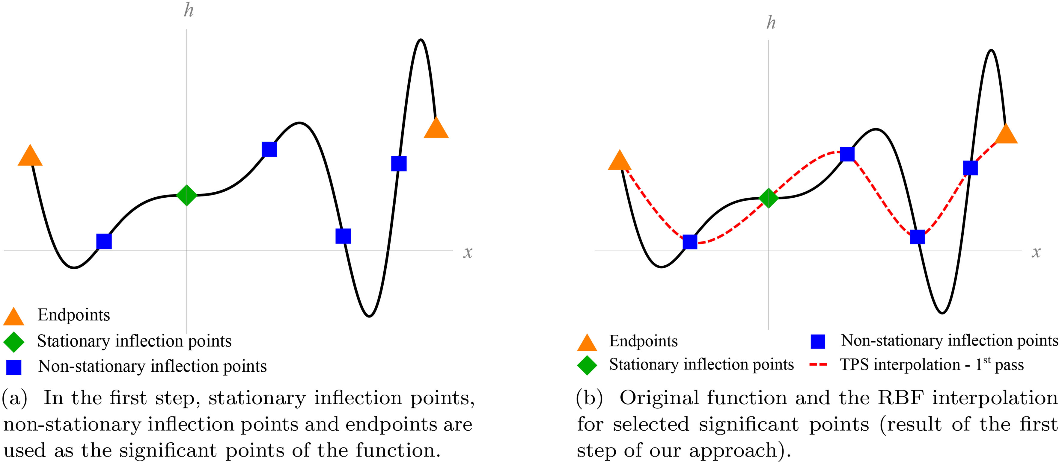
The local extrema, stationary and non-stationary inflection points and endpoints of the dataset are included among significant points, see Fig. 2a. The points which will be used for the determination of the set of significant points of the given data will be called the set of suspicious points $\{\bm{\psi}_{l}\}_{l=1}^{N_{S}}$ , i.e. a set of significant points is a reduced set of suspicious points.

First, the ordering of the given dataset is performed. After that, the set of suspicious points is determined. For these purposes, every four points $\{\bm{x}_{i},\dots,\bm{x}_{i+3}\}$ from the given data are interpolated by a cubic curve in the form:

$\displaystyle g_{q}(\bm{x})=\beta_{1q}\cdot\bm{x}^{3}+\beta_{2q}\cdot\bm{x}^{2% }+\beta_{3q}\cdot\bm{x}+\beta_{4q}$ (9) $\displaystyle q=1,\dots,N-3,$

which leads to the solution of the $(N-3)$ linear systems of the size $4\times 4$ . Then, the significant points $\{\bm{w}_{t}\}$ of this cubic are determined, see Fig. 2b. The significant points for the cubic curve Eq. (9) meet at least one of the following conditions:

$\displaystyle\frac{\partial g_{q}}{\partial\bm{x}}=0\ \text{or}\ \frac{% \partial^{2}g_{q}}{\partial\bm{x}^{2}}=0,$ (10)

which leads in our case to the following set:

$\displaystyle\left\{\bm{w}_{t}\right\}=\textstyle\left\{-\frac{\beta_{2q}}{3% \beta_{1q}}\right\}$ $\displaystyle\quad\cup\left\{\phantom{\frac{-\beta_{2q}\pm\sqrt{\beta_{2q}^{2}% -3\beta_{1q}\beta_{3q}}}{3\beta_{1q}}}\hskip-108.120472pt\left(\beta_{2q}^{2}-% 3\beta_{1q}\beta_{3q}\right)>0:\right.$ (11) $\displaystyle\quad\left.\frac{-\beta_{2q}\pm\sqrt{\beta_{2q}^{2}-3\beta_{1q}% \beta_{3q}}}{3\beta_{1q}}\right\}$

The significant point $\bm{w}_{t}$ is further added to the set of suspicious points $\{\bm{\psi}_{l}\}_{l=1}^{N_{S}}$ , if the necessary condition:

$\displaystyle\bm{x}_{i}\leqslant\bm{w}_{t}\leqslant\bm{x}_{i+3}$ (12)

is valid. Moreover, the functional value $g_{q}(\bm{\psi}_{l})$ of the associated cubic is calculated at such a suspicious point $\bm{\psi}_{l}$ :

$\displaystyle g_{q}(\bm{\psi}_{l})=\beta_{1q}\cdot\bm{\psi}_{l}^{3}+\beta_{2q}% \cdot\bm{\psi}_{l}^{2}+\beta_{3q}\cdot\bm{\psi}_{l}+\beta_{4q}$ (13)

and the absolute value of the first curvature $\left|{}^{1}k_{q}(\bm{\psi}_{l})\right|$ of the associated cubic is determined (using the symbolic manipulation):

$\displaystyle\left|{}^{1}k_{q}(\bm{\psi}_{l})\right|=\left|{}^{1}k\left(g_{q}(% \bm{\psi}_{l})\right)\right|==\textstyle\left|\frac{6\beta_{1q}\bm{\psi}_{l}+2% \beta_{2q}}{\left(1+\left(3\beta_{1q}\bm{\psi}_{l}^{2}+2\beta_{2q}\bm{\psi}_{l% }+\beta_{3q}\right)^{2}\right)^{3/2}}\right|.$ (14)

It should be noted that absolute values of the first curvature for the endpoints are calculated using the cubic curve interpolating points $\{\bm{x}_{1},\dots,\bm{x}_{4}\}$ , or $\{\bm{x}_{N-3},\ldots,\bm{x}_{N}\}$ .

0.3em0.8em 0.3em 0cm Determination of the set of significant points $\{\bm{\chi}_{u}\}_{1}^{S}$ , the absolute values of the first curvatures $\left\{\left|{}^{1}k(\bm{\chi}_{u})\right|\right\}_{1}^{S}$ and the associated functional values $\left\{g(\bm{\chi}_{u})\right\}_{1}^{S}$ .given points $\{\bm{x}_{i}\}_{1}^{N}\in\mathbb{E}^{1}$ and their associated scalar values $\{h_{i}\}_{1}^{N}\in\mathbb{E}^{1}$ , the average step between given sorted points $\delta$ significant points, their associated first curvatures and their associated functional values $\left\{\bm{\chi}_{u},\left|{}^{1}k(\bm{\chi}_{u})\right|,g(\bm{\chi}_{u})% \right\}_{1}^{S}$ Sort the given points $\{\bm{x}_{i}\}_{1}^{N}$ in ascending order. $i=1,\dots,N-3$ Determine the significant points $\left\{\bm{w}_{t}\right\}$ for cubic curve defined by $\{x_{i},\dots,x_{i+3}\}$ , (Eq. (9), Eq. (2.3)). $i=1$ Add the triplet $\left\{\bm{x}_{1},\left|{}^{1}k_{1}(\bm{x}_{1})\right|,h_{1}\right\}$ to the output (using Eq. (14)). $\bm{w}_{t}$ $\bm{x}_{i}\leqslant\bm{w}_{t}\leqslant\bm{x}_{i+3}$ Add the point $\bm{w}_{t}$ to the set of suspicious points $\{\bm{\psi}_{l}\}$ . Compute the first curvature $\left|{}^{1}k_{i}(\bm{w}_{t})\right|$ , eq. (14), and the functional value $g_{i}(\bm{w}_{t})$ , Eq. (13), and add these values to appropriate sets $i=(N-3)$ Add the triplet $\left\{\bm{x}_{N},\left|{}^{1}k_{N-3}(\bm{x}_{N})\right|,h_{N}\right\}$ to the output (using Eq. (14)). From the set of suspicious points $\{\bm{\psi}_{l}\}$ , delete all points such that Eq. (15) is valid. the set of suspicious points is not empty Find $\Psi_{u}=\left\{\bm{\psi}_{\hat{l}}:\|\bm{\psi}_{\hat{l}}-\bm{\psi}_{1}\|% \leqslant\delta\right\}$ in the set of suspicious points $\{\bm{\psi}_{l}\}$ . Add the triplet $\left\{\frac{\sum\bm{\psi}_{\hat{l}}}{|\Psi_{u}|},\frac{\sum\left|{}^{1}k_{q}(% \bm{\psi}_{\hat{l}})\right|}{|\Psi_{u}|},\frac{\sum g_{q}(\bm{\psi}_{\hat{l}})% }{|\Psi_{u}|}\right\}$ to the output ( $|\Psi_{u}|$ is cardinality of $\Psi_{u}$ ). Delete all points $\bm{\psi}_{\hat{l}}\in\Psi_{u}$ and their associated values from the sets $\{\bm{\psi}_{l}\}$ , $\left\{\left|{}^{1}k_{q}(\bm{\psi}_{l})\right|\right\}$ and $\left\{g_{q}(\bm{\psi}_{l})\right\}$ .

Figure 2.

Finding significant points of given data.

The set of suspicious points may contain two or more identical points or points very close to identical. This problem is caused by the fact that one significant point can be obtained from up to three cubics. Therefore, the reduction of the set of suspicious points is performed. The resulting set of significant points of the given data $\{\bm{\chi}_{u}\}$ is determined as follows. First, the endpoints are added to the set of significant points $\{\bm{\chi}_{u}\}$ , their associated functional values are added to set $\{g(\bm{\chi}_{u})\}$ and their associated absolute values of the first curvatures are added to set $\left\{\left|{}^{1}k(\bm{\chi}_{u})\right|\right\}$ . Now, let $\delta$ is the average step between the given sorted points, then the reduction of the set of suspicious points can be performed as follows. The suspicious points which meet the condition:

$\displaystyle\left(\|\bm{\psi}_{l}-\bm{x}_{1}\|\leqslant\delta\right)\text{or}% \left(\|\bm{\psi}_{l}-\bm{x}_{N}\|\leqslant\delta\right),$ (15)

are deleted. Further, the subset $\Psi_{u}$ of suspicious points, where each point meets the relation:

$\displaystyle\Psi_{u}=\left\{\bm{\psi}_{\hat{l}}:\|\bm{\psi}_{\hat{l}}-\bm{% \psi}_{1}\|\leqslant\delta\right\},$ (16)

is removed from the set of suspicious points $\{\bm{\psi}_{l}\}$ and the new significant point is determined from them by averaging:

$\displaystyle\bm{\chi}_{u}=\frac{\sum\bm{\psi}_{\hat{l}}}{|\Psi_{u}|},$ (17)

where $|\Psi_{u}|$ is a size (cardinality) of the subset $\Psi_{u}$ . Moreover, the associated functional value $g(\bm{\chi}_{u})$ and the associated absolute value of the first curvature $\left|{}^{1}k(\bm{\chi}_{u})\right|$ are determined in the same way. The process is repeated until the set of suspicious points is not empty.

The whole algorithm for finding the set of significant points of the given data, the calculation of the first curvatures and associated functional values in them is summarized in Algorithm 1.

3. Proposed two steps algorithm

In this section, the proposed two steps algorithm for the RBF approximation of the given data (in form $y=f(x)$ ) including the determination of placement of reference points and the derivation of an appropriate variable shape parameter will be described.

3.1 First step of the proposed approach

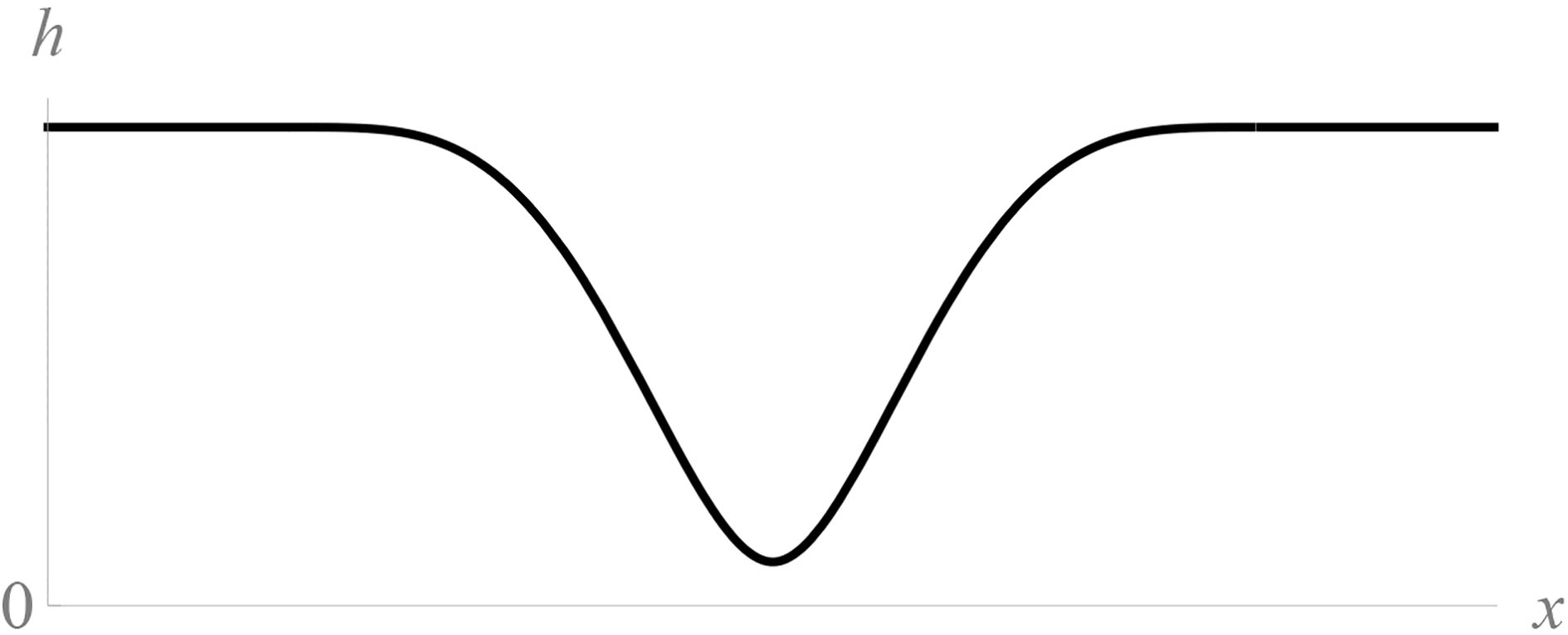
In this section, the first step of our approach will be described. The main goal of this step is to perform the primary RBF approximation of the given dataset such that the input data for the second step of our method will be symmetrically distributed around the $x$ -axis. This will be done using inflection points (stationary and non-stationary) and endpoints of the given data. Moreover, this step executes the shift of associated values $\{h_{i}\}_{1}^{N}$ so that the newly obtained associated values are better approximated using the RBF, i.e. the problematic course of the sampled function as in Fig. 3 will be eliminated.

Figure 3.

The course of the sampled function which is poorly approximated using the RBF.

Determination of shifted associated values $\{\hat{h}_{i}\}_{1}^{N}$ , i.e. the first step of the proposed approach. given points $\{\bm{x}_{i}\}_{1}^{N}$ and their associated scalar values $\{h_{i}\}_{1}^{N}$ interpolation points for the TPS interpolation $\{\bm{\hat{x}}_{v}\}_{1}^{M_{1}}$ , vector of weights for the TPS interpolation $\bm{c}_{I}$ , vector of coefficients for polynomial $\bm{a}_{I}$ and shifted associated values $\{\hat{h}_{i}\}_{1}^{N}$ Determine the significant points of the given data $\{\bm{\chi}_{u}\}_{1}^{S}$ and calculate the functional values and absolute values of the first curvatures in them, Algorithm 1. Add $\bm{\chi}_{1}$ to set $\{\bm{\hat{x}}_{v}\}$ and $g(\bm{\chi}_{1})$ to set $\{\hat{g}_{v}\}$ $u=2,\dots,S-1$ $\left|{}^{1}k(\bm{\chi}_{u})\right|$ is zero Add $\bm{\chi}_{u}$ to set $\{\bm{\hat{x}}_{v}\}$ and $g(\bm{\chi}_{u})$ to set $\{\hat{g}_{v}\}$ Add $\bm{\chi}_{S}$ to set $\{\bm{\hat{x}}_{v}\}$ and $g(\bm{\chi}_{S})$ to set $\{\hat{g}_{v}\}$ Compute the vector of weights $\bm{c}_{I}=(c_{I1},\ldots,c_{IM_{1}})$ and vector of polynomial coefficients $\bm{a}_{I}$ , Eq. (18) Compute shifted values $\hat{h}_{i}$ , where $i=1,\ldots,N$ , Eq. (3.1)

Figure 4.

The first step of our proposed method.

In the first step of our algorithm, the significant points of the given data $\{\bm{\chi}_{u}\}$ are firstly found using the method introduced in Section 2.3. From the set of significant points, only inflection points (stationary or non-stationary) and endpoints are used, see Fig. 4a.

Such a set of points is marked as $\{\bm{\hat{x}}_{v}\}_{1}^{M_{1}}$ , where $M_{1}$ is number of points of interest, and the set of their associated functional values is marked as $\{\hat{g}_{v}\}_{1}^{M_{1}}$ . The significant point $\bm{\chi}_{u}$ is an inflection point (stationary or non-stationary) if its associated absolute value of the first curvature $\left|{}^{1}k(\bm{\chi}_{u})\right|$ is zero (or close to zero).

Now, the RBF interpolation with polynomial reproduction [39] is performed for the set $\{\bm{\hat{x}}_{v}\}_{1}^{M_{1}}$ , where each point $\bm{\hat{x}}_{v}$ is associated with a value $\hat{g}_{v}$ , see Fig. 4b. This means that the vector of unknown weights $\bm{c}_{I}=(c_{I1},\dots,c_{IM_{1}})$ and vector of coefficients for the polynomial $\bm{a}_{I}$ are computed from the linear system of equations:

$\displaystyle\left(\begin{array}[]{cc}\bm{A}_{I}&\bm{P}_{I}\\ \bm{P}_{I}^{T}&\bm{0}\end{array}\right)\left(\begin{array}[]{c}\bm{c}_{I}\\ \bm{a}_{I}\end{array}\right)=\left(\begin{array}[]{c}\bm{h}\\ \bm{0}\end{array}\right),$ (18)

where the index $I$ means the interpolation case, the vector of associated values is $\bm{h}=(\hat{g}_{1},\dots,\hat{g}_{M_{1}})^{T}$ , the matrix $\bm{A}_{I}=\{A_{ij}\}=\left\{\phi_{\textit{TPS}}\left(\|\bm{\hat{x}}_{i}-\bm{% \hat{x}}_{j}\|\right)\right\}$ and the matrix $\bm{P}_{I}=\{P_{i}\}=\left\{\left(\bm{\hat{x}}_{i}^{T},1\right)\right\}$ .

The Thin-Plate Spline (TPS) is used as $\phi_{\textit{TPS}}$ , i.e.:

$\displaystyle\phi_{\textit{TPS}}(r)=r^{2}\log(r)=\frac{1}{2}\cdot r^{2}\log(r^% {2}).$ (19)

This global RBF is chosen because it is not dependent on a shape parameter.

When the vector of weights $\bm{c}_{I}$ and vector of coefficients $\bm{a}_{I}$ are determined, the new associated values (i.e. shifted associated values) for original dataset $\{\bm{x}_{i}\}_{1}^{N}$ can be computed:

$\displaystyle\hat{h}_{i}=h_{i}-\sum_{v=1}^{M_{1}}c_{Iv}\phi_{\textit{TPS}}% \left(\|\bm{x_{i}}-\bm{\hat{x}}_{v}\|\right)-P(\bm{x}_{i})$ $\displaystyle i=1,\dots,N,$ (20)

where $\phi_{\textit{TPS}}$ is given by Eq. (19).

The whole algorithm for the first step of the proposed approach, i.e. determination of shifted associated values $\{\hat{h}_{i}\}_{1}^{N}$ , is summarized in Algorithm 2.

3.2 Second step of the proposed approach

This section will be focused on the second step of our approach. In the input of this step, we assume that we have given the unordered dataset $\{\bm{x}_{i}\}_{1}^{N}\in\mathbb{E}^{1}$ and each point $\bm{x}_{i}$ from this dataset is associated with a shifted scalar value $\hat{h}_{i}$ (these values were calculated in the first step), see Fig. 5. Our goal is to determine the RBF approximation with a variable shape parameter and Lagrange multipliers for the described data. Therefore, the set of reference points has to be determined. It should be noted that the placement of reference points has a significant influence on the quality of the approximation. If the reference points are located at the significant points of the given data, then better approximation results are obtained.

Figure 5.

Course of the input sampled function for the second step of the proposed approach. The set of reference points for the second step of our approach are marked. Hexagons indicate input points for the TPS interpolation from the first step (i.e. stationary and non-stationary inflection points and endpoints) and circles denote local extrema of shifted functional values.

Therefore, the significant points $\left\{\bm{\hat{\chi}}_{u}\right\}$ of the input data for the second step are found using the method which was introduced in Section 2.3. This set of significant points is further used as the reference points of the RBF approximation $\{\bm{\xi}_{j}\}_{1}^{M}$ . It should be noted that the inflection points (stationary and non-stationary) and endpoints from the second step correspond to the input points for the TPS interpolation $\displaystyle\{\bm{\hat{x}}_{v}\}_{1}^{M_{1}}$ from the first step, i.e. only local extrema are newly added, see Fig. 5.

3.3 Determination of appropriate variable shape parameter

The variable shape parameters of RBF $\alpha_{j}$ at appropriate reference points $\bm{\xi}_{j}$ can be determined when the reference points and absolute values of the first curvatures in them are known. Our approach for determining the variable shape parameters is based on a requirement that the validity of the following equality is required:

$\displaystyle\left(\hat{h}_{max}-\hat{h}_{min}\right)\cdot\left|{}^{1}k_{\phi}% (0,\alpha_{j})\right|$

(21) $\displaystyle\quad=\left|\phi(0)\right|\cdot\left|{}^{1}k(\bm{\xi}_{j})\right|,$

where $\hat{h}_{\textit{max}}=\max_{i=1,\ldots,N}(\hat{h}_{i})$ is the maximum of shifted associated values and $\hat{h}_{\textit{min}}=\min_{i=1,\ldots,N}(\hat{h}_{i})$ is the minimum of shifted associated values, $\phi(0)$ is the value of the radial basis function at the center, $|^{1}k_{\phi}(0,$ $\alpha_{j})|$ is the absolute value of the first curvature for radial basis function $\phi(\|\bm{x}-\bm{\xi}_{j}\|)$ at point $\bm{x}=\bm{\xi}_{j}$ . The above mentioned equality is derived based on the consideration that the RBF curve centered at reference point $\bm{\xi}_{j}$ has the greatest influence from all used RBFs on the shape of the approximating function at this point, and therefore, the match of the absolute value of first curvature is required. Moreover, the normalization of both function is taken to account. The absolute value of the first curvature for the RBF curve centered at reference point $\bm{\xi}_{j}$ is obtained as:

$\displaystyle\left|{}^{1}k_{\phi}(r,\alpha_{j})\right|=\left|\frac{\phi_{rr}(r% ,\alpha_{j})}{(1+\phi_{r}^{2}(r,\alpha_{j}))^{3/2}}\right|,$ (22)

where $\phi_{rr}(r,\alpha_{j})$ denotes the second derivative and $\phi_{r}(r,\alpha_{j})$ denotes the first derivative of the RBF.

From equality Eq. (3.3), the following equation can be derived for variable shape parameter $\alpha_{j}$ of the RBF:

$\displaystyle\alpha_{j}=\frac{1}{2}\sqrt{\frac{\left|{}^{1}k(\bm{\xi}_{j})% \right|\cdot\left|\phi(0)\right|}{\omega\cdot\left(\hat{h}_{\textit{max}}-\hat% {h}_{\textit{min}}\right)}},$ (23)

where $\hat{h}_{\textit{max}}$ is the maximum of shifted values, $\hat{h}_{\textit{min}}$ is the minimum of shifted values, $\left|{}^{1}k(\bm{\xi}_{j})\right|$ is the associated absolute value of the first curvature, which was determined by the algorithm described in Section 2.3, and $\omega$ is a constant parameter depending on the type of RBF used, see Table 1.

Table 1
Different RBFs and their parameter $\omega$ , e.g. Eq. (23)

RBF $\bm{\phi}(\bm{r})$ $\bm{\omega}$

Gaussian RBF $e^{-(\alpha r)^{2}}$ 2

Inverse quadric $\frac{1}{1+(\alpha r)^{2}}$ 2

Wendland’s $\phi_{3,2}$ $(1-\mathnormal{\alpha}r)_{+}^{6}(35(\alpha r)^{2}+18\alpha r+3)$ 56

It should be noted that this approach can be used only for RBFs which have smoothness of at least $C^{3}$ at the origin, because the first curvature of the RBF curve should be smooth.

The last problem which has to be solved is the case when shape parameter $\alpha_{j}$ associated with reference point $\bm{\xi}_{j}$ is zero (i.e. the reference point is an inflection point of the given data), because for such shape parameter the constant function would be obtained. In these cases, correction of the shape parameter is made. Specifically, the weighted average of shape parameters associated with the neighboring points is established and is used as the value of shape parameter $\alpha_{j}$ .

The whole algorithm for determination of appropriate variable shape parameters is summarized in Algorithm 3.

Determination of the variable shape parameters $\alpha_{j}$ at appropriate reference points $\bm{\xi}_{j}$ . reference points and their associated absolute values of the first curvatures $\left\{\bm{\xi}_{j},\left|{}^{1}k(\bm{\xi}_{j})\right|\right\}_{1}^{M}$ , the minimum of shifted associated values $\hat{h}_{\textit{min}}=\min_{i=1,\dots,N}(\hat{h}_{i})$ , the maximum of shifted associated values $\hat{h}_{\textit{max}}=\max_{i=1,\dots,N}(\hat{h}_{i})$ and the coefficient $\omega$ for used RBF (see Table 1) variable shape parameters associated with appropriate reference points $\{\alpha_{j}\}_{1}^{M}$ Sort the given pairs $\left\{\bm{\xi}_{j},\left|{}^{1}k(\bm{\xi}_{j})\right|\right\}_{1}^{M}$ in ascending order with respect to coordinates of reference points. $j=1,\dots,M$ $\alpha_{j}=\frac{1}{2}\sqrt{\frac{\left|{}^{1}k(\bm{\xi}_{j})\right|\cdot|\phi% (0)|}{(h_{\textit{max}}-h_{\textit{min}})\cdot\omega}}$ $j=1,\ldots,M$ $\alpha_{j}$ is zero $j=1$ $\alpha_{j}=\alpha_{j+1}$ $j=M$ $\alpha_{j}=\alpha_{j-1}$ $\alpha_{j}=\frac{\alpha_{j-1}\cdot\|\bm{\xi}_{j}-\bm{\xi}_{j-1}\|+\alpha_{j+1}% \cdot\|\bm{\xi}_{j+1}-\bm{\xi}_{j}\|}{\|\bm{\xi}_{j+1}-\bm{\xi}_{j-1}\|}$
3.4 Algorithm summary

RBF	$\bm{\phi}(\bm{r})$	$\bm{\omega}$
Gaussian RBF	$e^{-(\alpha r)^{2}}$	2
Inverse quadric	$\frac{1}{1+(\alpha r)^{2}}$	2
Wendland’s $\phi_{3,2}$	$(1-\mathnormal{\alpha}r)_{+}^{6}(35(\alpha r)^{2}+18\alpha r+3)$	56

In this section, a summary of the whole proposed algorithm is provided. First, the first step of the proposed approach is performed, see Algorithm 2, i.e. the TPS interpolation and shift of associated values $\left\{\hat{h}_{i}\right\}_{1}^{N}$ are determined, which leads to the elimination of the problematic course of the sampled function. Next, the reference points $\{\bm{\xi}_{j}\}_{1}^{M}$ are found and their appropriate absolute values of the first curvatures are calculated for the newly determined data, see Algorithm 1. Then, the appropriate variable shape parameters $\{\alpha_{j}\}_{1}^{M}$ are computed, see Algorithm 3. After that, the RBF approximation can be performed. For these purposes, the RBF approximation with a variable shape parameter and Lagrange multipliers, see Section 2.2, is used. Therefore, the constraints (see Eq. (5)) have to be defined. For the proposed approach, the following constraints are used:

$\displaystyle\left\{f(\bm{x}_{1})=\hat{h}_{1}=0,\enspace f(\bm{x}_{N})=\hat{h}% _{N}=0\right\},$ (24)

i.e. the given values $\left\{s_{k}\right\}=\left\{0,0\right\}$ have to be strictly respected at endpoints $\left\{\bm{\eta}_{k}\right\}=\left\{\bm{x}_{1},\bm{x}_{N}\right\}$ . Now, using Eq. (8), the vector of unknown weights $\bm{c}=\left(c_{1},\dots,c_{M}\right)^{T}$ can be determined.

Finally, the approximated value is determined as:

$\displaystyle f(\bm{x})=\sum_{v=1}^{M_{1}}c_{Iv}\phi_{\textit{TPS}}\left(\|\bm% {x}-\bm{\hat{x}}_{v}\|\right)+P(\bm{x})+\sum_{j=1}^{M}c_{j}\phi\left(\|\bm{x}-% \bm{\xi}_{j}\|,\alpha_{j}\right),$ (25)

where $\bm{c}_{I}=(c_{I1},\dots,c_{IM_{1}})$ is the vector of weights for the TPS interpolation, $\phi_{\textit{TPS}}$ is the Thin-Plate-Spline, $\{\bm{\hat{x}}_{v}\}_{1}^{M_{1}}$ are input points for the TPS interpolation, $M_{1}$ is number of interpolation points for the first step, $P(\bm{x})$ is polynomial function of first order, $\bm{c}=(c_{1},\dots,c_{M})$ is the vector of weights for the RBF approximation, $\phi$ is the RBF used (see Table 1), $\{\bm{\xi}_{j}\}_{1}^{M}$ is the set of reference points, $M$ is number of reference points for the second step and $\{\alpha_{j}\}_{1}^{M}$ are appropriate variable shape parameters.

4. Experimental results

The above-proposed method of the RBF approximation has been tested on different datasets using Matlab. Moreover, a comparison with the RBF approximation using the constant shape parameter for different distributions of the set of reference points has been made using different radial basis functions, see Table 1.

4.1 Distribution of reference points

For the comparison of our approach, the following sets of reference points were used:

Uniform points:
This set contains the points distribu-ted uniformly at a given interval.
Epsilon points:
This is a special distribution of points which is based on uniform points. Specifically, the points from uniform distribution are randomly drift about value from a range $(-\varepsilon_{x},\varepsilon_{x})$ , where $\varepsilon_{x}$ responds to a quarter of the step of uniform points.
Optimal points:
The set of reference points from the second step of the proposed approach is used.

Table 2
Experimental setups – $\{h_{i}\}_{i=1}^{N}$ indicates the sampling function of the associated values, $N$ is size of input dataset, $M_{1}$ is number of interpolation points for the first step, $M$ is number of reference points for the second step and $\phi(r)$ is RBF used

${\{h_{i}\}_{i=1}^{N}}$ ${N}$ ${M_{1}}$ ${M}$ ${\phi}(\bm{r})$

Experiment no. 1 $f_{1}$ , Eq. (26) 200 7 13 Gaussian RBF

Experiment no. 2 $f_{2}$ , Eq. (27) 200 7 13 Inverse quadric

Experiment no. 3 $f_{3}$ , Eq. (28) 200 6 11 Wendland’s $\phi_{3,2}$

4.2 Testing datasets

	${\{h_{i}\}_{i=1}^{N}}$	${N}$	${M_{1}}$	${M}$	${\phi}(\bm{r})$
Experiment no. 1	$f_{1}$ , Eq. (26)	200	7	13	Gaussian RBF
Experiment no. 2	$f_{2}$ , Eq. (27)	200	7	13	Inverse quadric
Experiment no. 3	$f_{3}$ , Eq. (28)	200	6	11	Wendland’s $\phi_{3,2}$

A uniform distribution of points was used for the testing data. The given dataset contains 200 points uniformly distributed in the interval $[0,1]$ . Moreover, each point from this dataset is associated with a function value at this point. For this purpose, many different functions have been used. Results for some representative functions are presented below.

$\displaystyle f_{1}(x)=\sin{\left(15x^{2}\right)}+5x$ (26) $\displaystyle f_{2}(x)=(4.88x-1.88)\cdot\sin{\left((4.88x-1.88)^{2}\right)}+1$ (27) $\displaystyle f_{3}(x)=e^{10x-6}\cdot\sin{\left((5x\!-\!2)^{2}\right)}\!+\!(3x% \!-\!1)^{3}$ (28)

4.3 Experimental results and comparisons

The experimental results for the proposed approach will be presented and their comparison with results for another RBF approximation using the constant shape parameter for different distributions of reference points will be made. The shape parameters $\alpha$ for the RBFs used, in the case of approximation with the constant shape parameter, were determined experimentally with regard to the quality of the approximation, i.e. they were selected the shape parameters $\alpha$ for which the lowest mean absolute error of the approximation was obtained. Moreover, the RBF approximation using the constant shape parameter was applied in two ways. The first one is that the RBF approximation with the constant shape parameter was performed for the original input data. The second one is that the original input data was preprocessed and then the RBF approximation with the constant shape parameter was applied. This preprocessing consists of the application of the first step from the proposed approach to the original input data, i.e. the RBF approximation using the constant shape parameter is applied to shifted data. The setups for presented experiments are presented in Table 2.

Table 3
The RBF approximation error for the tested datasets and different initial configurations

Experiment no. 1
		Original data			Shifted data
Phenomenon	Proposed approach	Uniform ref. pts.	Epsilon ref. pts.	Optimal ref. pts.	Uniform ref. pts.	Epsilon ref. pts.	Optimal ref. pts.
Mean absolute error	3.13E-03	8.55E-03	8.20E-03	6.21E-03	1.23E-02	1.22E-02	9.09E-03
Deviation of error	3.71E-06	1.01E-04	7.56E-05	2.11E-05	1.74E-04	1.62E-04	1.48E-04
Mean relative error	1.17E-03	3.18E-03	3.05E-03	2.31E-03	4.59E-03	4.54E-03	3.38E-03
Experiment no. 2
Mean absolute error	9.49E-03	1.80E-02	1.77E-02	1.18E-02	2.23E-02	2.23E-02	1.52E-02
Deviation of error	9.94E-05	5.24E-04	6.09E-04	1.37E-04	5.51E-04	6.06E-04	1.21E-04
Mean relative error	7.94E-03	1.51E-02	1.48E-02	9.83E-03	1.86E-02	1.86E-02	1.27E-02
Experiment no. 3
Mean absolute error	7.52E-02	2.04E+00	1.98E+00	8.12E-02	2.14E+00	2.37E+00	1.45E-01
Deviation of error	8.62E-03	1.37E+01	1.48E+01	2.18E-02	1.67E+01	1.58E+01	4.79E-02
Mean relative error	1.75E-02	4.74E-01	4.61E-01	1.89E-02	4.98E-01	5.52E-01	3.37E-02

Figure 6.

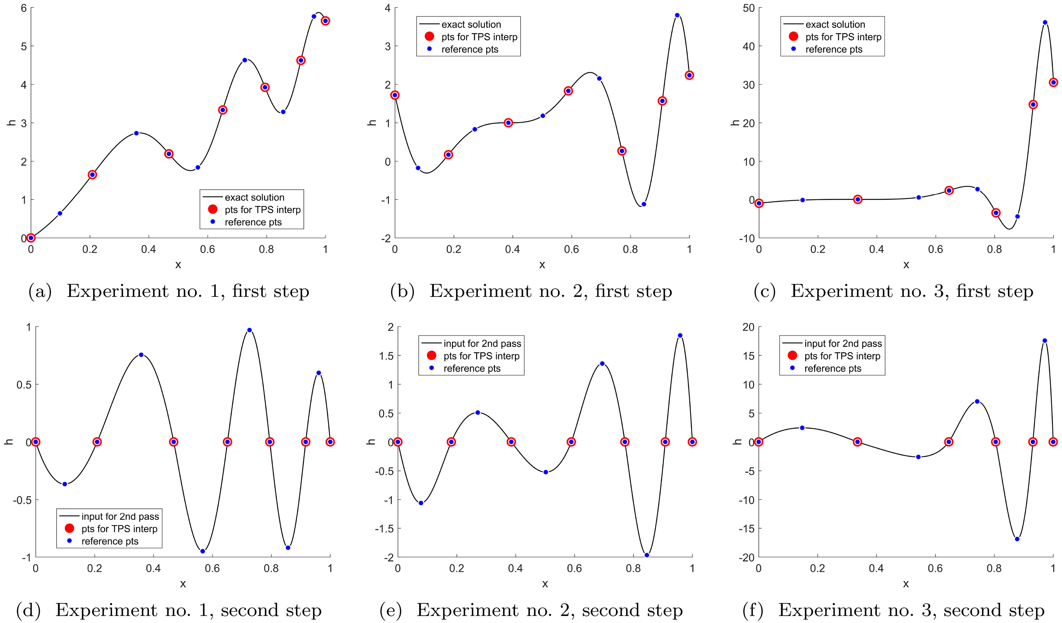
Trends of input data for the first step (top) and trends of input data for the second step (bottom) for different experiments, see Table 2. The sets of reference points for both steps are marked.

Figure 7.

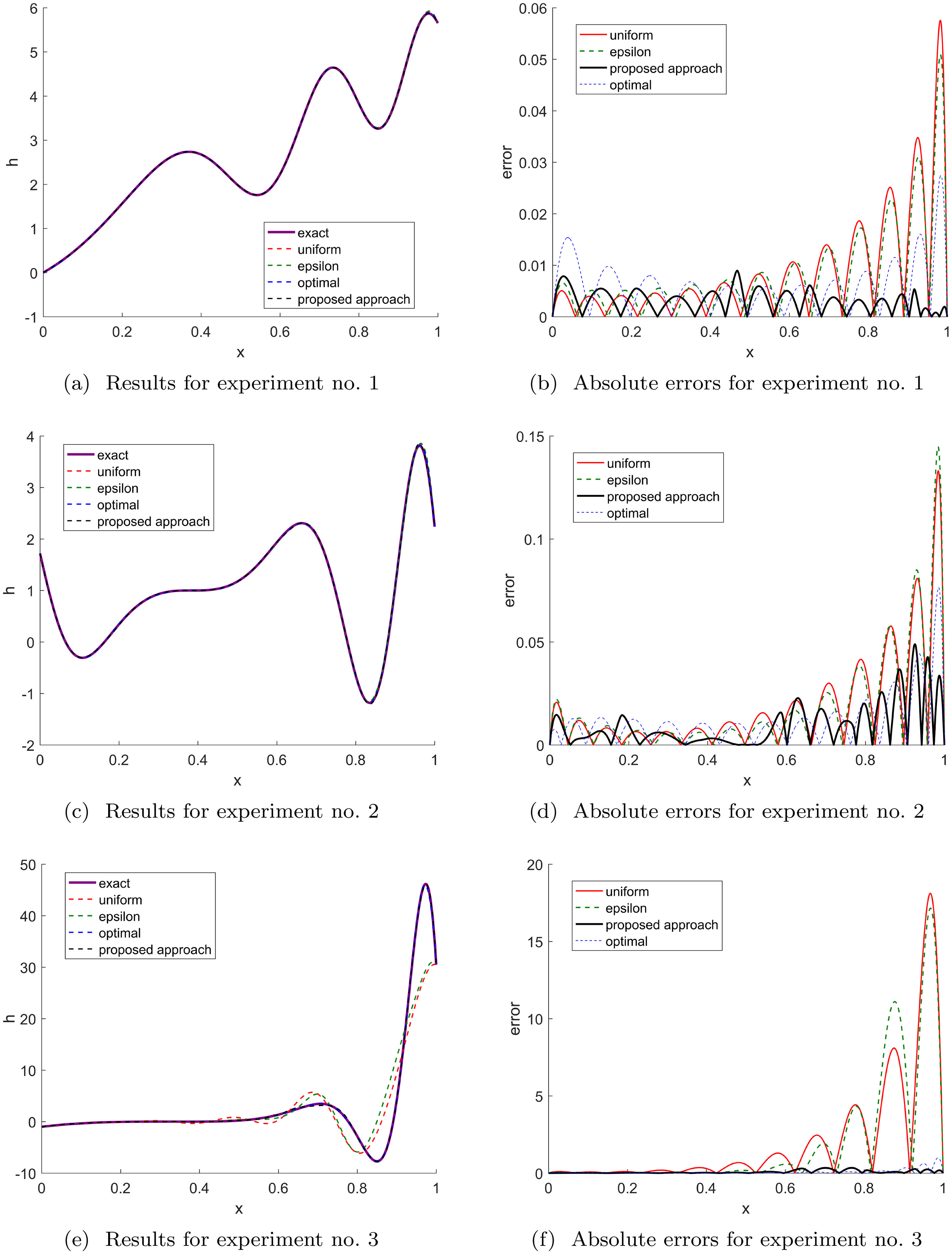
Results of the RBF approximation (left) and their errors (right) for different initial configurations and different experiments, see Table 2. The RBF approximation with the constant shape parameter is applied to the original data, i.e. the preprocessing is not included. The initial configurations are: constant shape parameter and uniform reference points (uniform), constant shape parameter and epsilon reference points (epsilon), constant shape parameter and optimal reference points (optimal) and the proposed approach (note that values of the proposed method are nearly equal to the exact ones).

Figure 8.

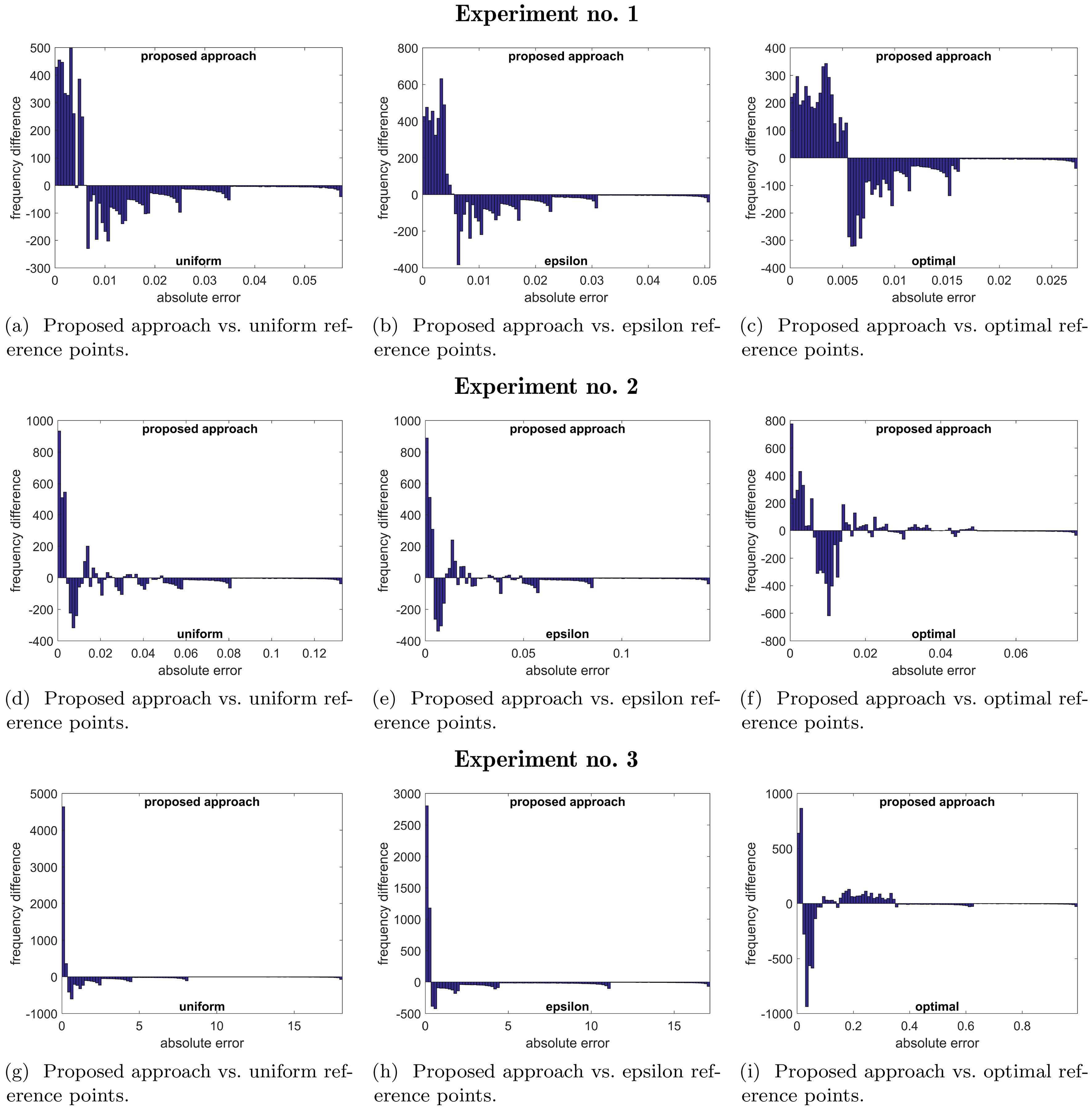
Difference histograms of approximation errors for different experiments, see Table 2. The RBF approximation with the constant shape parameter is applied to the original data, i.e. the preprocessing is not included.

The trends of the original data for the different experiments from Table 2 are shown in Fig. 6 (top). Figure 7 presents the results for the different experiments in which each point is associated with a value from some sampling function Eqs (26)–(28) and some RBF from Table 1 is used. The specific choice of the sampling function and RBF for each experiment is mentioned in Table 2. Using the proposed approach, $M$ significant points (see Table 2) were found for the chosen datasets and $M_{1}$ of them (see Table 2) were classified as inflection points or endpoints. These $M_{1}$ significant points were used for the TPS interpolation in the first step. The trends of the data after the first step, i.e. after performing the shift of associated values, can be seen in Fig. 6 (bottom) for the different experiments from Table 2. The points for the TPS interpolation from the first step and reference points used for the second step for the different experiments are visualized in Fig. 6 (bottom) on the shifted data and in Fig. 6 (top) on the original data.

Figure 9.

Recovering the smooth robot trajectory from real data [40] using the proposed RBF approximation ( $N=$ 407 – number of given points for both curves $x(t)$ and $y(t)$ , $M_{1x}=$ 38 and $M_{1y}=$ 28 – number of points for the TPS interpolation, $M_{x}=$ 63 and $M_{y}=$ 50 – number of reference points for the second step of the proposed algorithm.

Figure 10.

Result of the proposed RBF approximation for real dataset which represents the terrain profile ( $N=$ 2711 – number of given points, $M_{1}=$ 30 – number of points for the TPS interpolation and $M=$ 55 number of reference points for the second step of the proposed algorithm).

Figure 7 (left), in addition to the RBF approximation using the proposed approach, also presents the results of the RBF approximation using the constant shape parameter, where the set of reference points has uniform, epsilon or optimal distribution and contains $M$ points (see Table 2). In this case, the RBF approximation using the constant shape parameter was applied to the original input data, i.e. the preprocessing is not included. The magnitudes of error for these approximations can be seen in Fig. 7 (right). The error is defined as the absolute value of the difference between the sampling function, some of the Eqs (26)–(28), and the approximated function. The differences of frequencies of errors for different experiments are shown in Fig. 8. Moreover, the three basic error measures (mean absolute error, deviation of error and mean relative error) for all experiments mentioned are shown in Table 3. It can be observe that the proposed approach returns better results than the other methods in terms of the error.

The results of comparison of the proposed approach with the RBF approximation using the constant shape parameter for different distributions of the set of reference points and different experiments from Table 2 when the preprocessing was used, i.e. the approximation was applied to shifted data, see Fig. 6 (bottom), have the similar visual results as when the preprocessing is not included, and therefore, these experiments are presented only by the three basic error measures, see Table 3.

The proposed algorithm was applied on data for recovering smooth robot trajectory in the space which can be computed as the curve parameterized by time. Description of results for this experiment follows. The two separate functions, $x(t)$ and $y(t)$ , each representing its respective coordinate and depending on time $t$ on which the proposed algorithm was used, are shown in Fig. 9(a). These two functions are represented the parametric curve which is presented together with the original data in Fig. 9(b). The histograms of absolute errors for both functions $x(t)$ and $y(t)$ when the proposed approach is used can be seen in Fig. 9(c). Finally, the differences of frequencies of errors for comparison with the RBF approximation using the constant shape parameter for uniform distribution of set of reference points is presented in Fig. 9(d)–(e). It can be seen that the proposed approach returns better results than the other methods in terms of the error. Moreover, the proposed algorithm is able to reconstruct and smoothly connect a path even if data is missing for a certain period of time. It should be noted that the smooth connection of path is the key property for robot path planning.

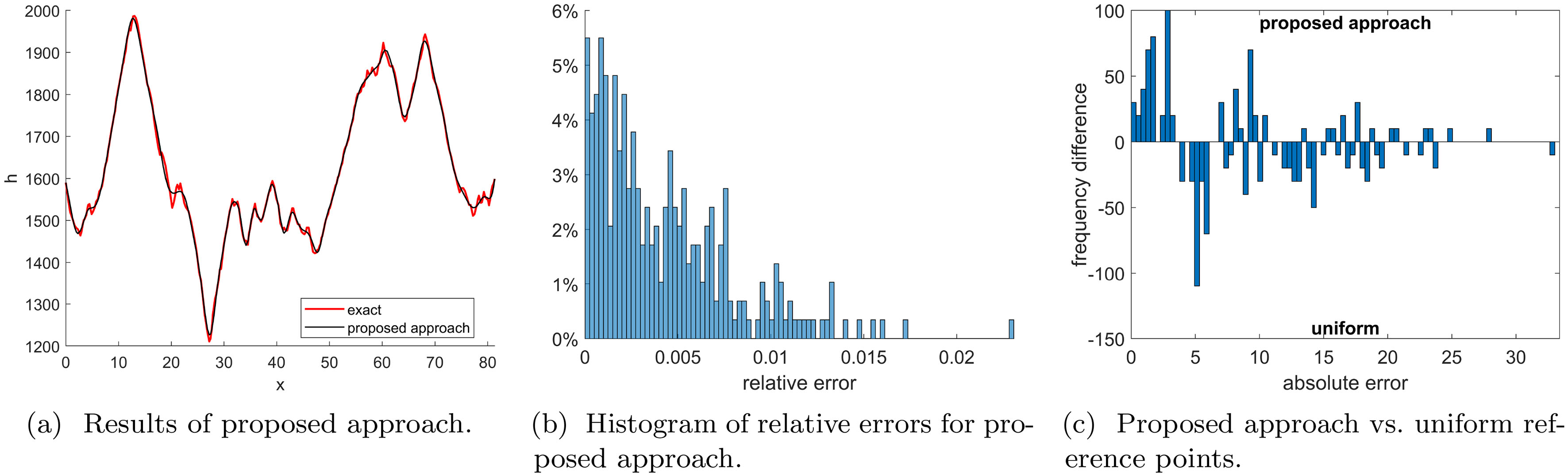
Further, the application of the proposed approach on real dataset which represents the terrain profile (2711 points) was performed and the comparison with the RBF approximation using the constant shape parameter for uniform distribution of the set of reference points is presented, see Fig. 10.

It can be seen that the proposed approach can well approximate the global trend of terrain profile for a small set of reference points. The further improving of result could be obtained e.g. by application of some incremental method. Moreover, it can be seen that the proposed approach returns again better results than the other methods in terms of the error.

It can be concluded that the RBF approximation for which the distribution of the set of reference points does not reflect the features of the approximated data and the number of reference points is minimal in terms of usability, i. e. uniform and epsilon distribution in our experiments, returns much worse results than the approximation for which features of the given data are reflected.

5. Conclusion

In this paper, a new algorithm for the radial basis function (RBF) approximation of functions $y=f(x)$ with the variable and adaptive shape parameter based on curve curvature behavior is presented. The proposed method has two steps based on exploiting features of the given dataset, such as extreme points and inflection points. The first step of the proposed approach is applying the global RBF interpolation of the selected subset of significant points, which leads to an adaptive shift of the given data in terms of associated values. After that, the RBF approximation with the variable shape parameter is performed on modified data. The set of reference points is derived using significant points of the shifted data and the variable shape parameters are determined according to the first curvature in them.

The experiments proved that the proposed method gives significantly better results over other relevant competing methods. Moreover, it can be observed that the RBF approximation for which features of the given data are not respected is not capable of competing with the RBF approximation respecting data features, especially when the number of reference points is small.

The proposed method significantly eliminates problems with a shape parameter estimation inherited from the RBF’s general properties. The proposed algorithm can be used for the RBF approximation of a curve which is parameterized by one variable in multidimensional space. In future, the proposed approach is to be extended for explicit functions of two variables, i.e. to higher dimensions.

Footnotes

Acknowledgments

The authors would like to thank their colleagues at the University of West Bohemia, Plzeň, for their discussions and suggestions. The research was supported by the Czech Science Foundation GAČR project GA17-05534S and partially supported by the SGS 2019-016 project.

References

Hardy

. Multiquadratic Equations of Topography and Other Irregular Surfaces. Journal of Geophysical Research. 1971; 76: 1905-1915.

Hardy

. Theory and applications of the multiquadric-biharmonic method 20 years of discovery 1968–1988. Computers & Mathematics with Applications. 1990; 19(8): 163-208.

Pepper

Rasmussen

Fyda

. A meshless method using global radial basis functions for creating 3-D wind fields from sparse meteorological data. Computer Assisted Methods in Eng & Science. 2014; 21(3-4): 233-243.

Carr

Beatson

Cherrie

Mitchell

Fright

McCallum

, et al. Reconstruction and representation of 3D objects with radial basis functions. In: SIGGRAPH 2001. ACM; 2001. pp. 67-76.

Majdisova

Skala

. Big geo data surface approximation using radial basis functions: A comparative study. Computers & Geosciences. 2017; 109: 51-58.

Smolik

Skala

. Large scattered data interpolation with radial basis functions and space subdivision. Integrated Computer-Aided Engineering. 2018; 25(1): 49-62.

Smolik

Skala

Majdisova

. Vector field radial basis function approximation. Advances in Engineering Software. 2018; 123: 117-129.

Hon

Šarler

Yun

. Local radial basis function collocation method for solving thermo-driven fluid-flow problems with free surface. Engineering Analysis with Boundary Elements. 2015; 57: 2-8.

Chen

. The localized RBFs collocation methods for solving high dimensional PDEs. Engineering Analysis with Boundary Elements. 2013; 37(10): 1300-1304.

10.

Wendland

. Computational aspects of radial basis function approximation. Studies in Computational Mathematics. 2006; 12: 231-256.

11.

Fasshauer

Zhang

. On choosing “optimal” shape parameters for RBF approximation. Numerical Algorithms. 2007; 45(1-4): 345-368.

12.

Gherlone

Iurlaro

Sciuva

. A novel algorithm for shape parameter selection in radial basis functions collocation method. Composite Structures. 2012; 94(2): 453-461.

13.

Huang

Lee

Cheng

AHD

. Error estimate, optimal shape factor, and high precision computation of multiquadric collocation method. Engineering Analysis with Boundary Elements. 2007; 31(7): 614-623.

14.

Scheuerer

. An alternative procedure for selecting a good value for the parameter c in RBF-interpolation. Adv Comput Math. 2011; 34(1): 105-126.

15.

Zhu

Wathen

. Convexity and Solvability for Compactly Supported Radial Basis Functions with Different Shapes. Journal of Scientific Computing. 2015; 63(3): 862-884.

16.

Bozzini

Lenarduzzi

Rossini

Schaback

. Interpolation with variably scaled kernels. IMA Journal of Numerical Analysis. 2015; 35(1): 199-219.

17.

Afiatdoust

Esmaeilbeigi

. Optimal variable shape parameters using genetic algorithm for radial basis function approximation. Ain Shams Engineering Journal. 2015; 6(2): 639-647.

18.

Sanyasiraju

YVSS

Satyanarayana

. On optimization of the RBF shape parameter in a grid-free local scheme for convection dominated problems over non-uniform centers. Applied Mathematical Modelling. 2013; 37(12): 7245-7272.

19.

Bozzini

Lenarduzzi

Schaback

. Adaptive Interpolation by Scaled Multiquadrics. Advances in Computational Mathematics. 2002; 16(4): 375-387.

20.

Kansa

Carlson

. Improved accuracy of multiquadric interpolation using variable shape parameters. Computers & Mathematics with Applications. 1992; 24(12): 99-120.

21.

Cheng

Zhang

Caraffini

Neri

. Multicriteria adaptive differential evolution for global numerical optimization. Integrated Computer-Aided Engineering. 2015; 22(2): 103-107.

22.

Rostami

Neri

. Covariance matrix adaptation pareto archived evolution strategy with hypervolume-sorted adaptive grid algorithm. Integrated Computer-Aided Engineering. 2016; 23(4): 313-329.

23.

Rostami

Neri

Epitropakis

. Progressive preference articulation for decision making in multi-objective optimisation problems. Integrated Computer-Aided Engineering. 2017; 24(4): 315-335.

24.

Biazar

Hosami

. Selection of an interval for variable shape parameter in approximation by radial basis functions. Advances in Numerical Analysis. 2016; 2016.

25.

Ranjbar

. A new variable shape parameter strategy for Gaussian radial basis function approximation methods. Annals of the University of Craiova-Mathematics and Computer Science Series. 2015; 42(2): 260-272.

26.

Martynova

. A Novel Approach of the Approximation by Patterns Using Hybrid RBF NN with Flexible Parameters. In: CoMeSySo 2018; Springer; 2019. pp. 225-235.

27.

Adeli

Karim

. Fuzzy-wavelet RBFNN model for freeway incident detection. Journal of Transportation Engineering. 2000; 126(6): 464-471.

28.

Karim

Adeli

. Comparison of Fuzzy-Wavelet Radial Basis Function Neural Network Freeway Incident Detection Model with California Algorithm. Journal of Transportation Engineering. 2002; 128(1): 21-30.

29.

Karim

Adeli

. Radial basis function neural network for work zone capacity and queue estimation. Journal of Transportation Engineering. 2003; 129(5): 494-503.

30.

Ghosh-Dastidar

Adeli

Dadmehr

. Principal component analysis-enhanced cosine radial basis function neural network for robust epilepsy and seizure detection. IEEE Tran on Biomedical Eng. 2008; 55(2): 512-518.

31.

Chen

Cowan

CFN

Grant

. Orthogonal least squares learning algorithm for radial basis function networks. IEEE Transactions on Neural Networks. 1991; 2(2): 302-309.

32.

Chen

Franti

. Compression of GPS Trajectories. In: DCC 2012; IEEE; 2012. pp. 62-71.

33.

Aleotti

Caselli

Maccherozzi

. Trajectory reconstruction with NURBS curves for robot programming by demonstration. In: 2005 International Symposium on Computational Intelligence in Robotics and Automation. IEEE; 2005. pp. 73-78.

34.

Tian

Dong

Zeng

Long

Lin

, et al. Theoretical Analysis and Verification of Time Variation of Background Ionosphere on Geosynchronous SAR Imaging. IEEE Geoscience and Remote Sensing Letters. 2015; 12(4): 721-725.

35.

Majdisova

Skala

. Radial basis function approximations: comparison and applications. Applied Mathematical Modelling. 2017; 51: 728-743.

36.

Skala

. Fast Interpolation and Approximation of Scattered Multidimensional and Dynamic Data Using Radial Basis Functions. WSEAS Transactions on Mathematics. 2013; 12(5): 501-511.

37.

Skala

. RBF Approximation of Big Data Sets with Large Span of Data. In: MCSI 2017; IEEE; 2017. pp. 212-218.

38.

Fornberg

Zuev

. The Runge phenomenon and spatially variable shape parameters in RBF interpolation. Computers & Mathematics with Applications. 2007; 54(3): 379-398.

39.

Skala

. RBF Interpolation with CSRBF of Large Data Sets. Procedia Computer Science. 2017; 108: 2433-2437. ICCS 2017.

40.

Blanco

Moreno

González

. A Collection of Outdoor Robotic Datasets with centimeter-accuracy Ground Truth. Autonomous Robots. 2009; 27(4): 327-351.

Algorithm for placement of reference points and choice of an appropriate variable shape parameter for the RBF approximation

Abstract

Keywords

1. Introduction

2. Theoretical background

2.1 RBF approximation with a variable shape parameter

3.1 First step of the proposed approach

4.1 Distribution of reference points

Table 3 The RBF approximation error for the tested datasets and different initial configurations

Footnotes

Acknowledgments

References

Table 3
The RBF approximation error for the tested datasets and different initial configurations