
Abstract
In recent years, incremental sampling-based motion planning algorithms have been widely used to solve robot motion planning problems in high-dimensional configuration spaces. In particular, the Rapidly-exploring Random Tree (RRT) algorithm and its asymptotically-optimal counterpart called RRT
Introduction
The development of modern autonomous robots poses difficult tasks associated with the interaction between the robot and the external world, see [25, 64]. For example, a shape reconstruction system of 3D objects is proposed in [68] and a vision based navigation system for drones is proposed in [5]. Several studies on the modelling of the artificial visual system have been performed, e.g. a neural model [40] and methods on the functioning of artificial compound eye in [74, 73]. The task of detecting and interpreting a moving object, that is motion tracking, is fundamental for the correct functioning of a robot [8, 76].
This article studies a crucially important problem related to motion tracking, i.e. motion planning. The motion planning problem consists of finding a trajectory to move an agent trough a complex environment from a starting point to a desired area avoiding any obstacle while considering constraints related to the agent such as shape, kinematics and others. This problem is critical in almost all robot applications since, by definition, a robot is a machine developing tasks in the real world. Furthermore, this problem is also relevant in many other research areas such as verification, computational biology, and computer animation [34]. The first computational complexity results for robot motion planning were due to Reif [63]. Specifically, he established that the cited problem is PSPACE-hard when the final positions of the obstacles are specified. Moreover, this problem belongs to the class PSPACE when it is expressed using polynomials with rational coefficient [12], that is, this variant is a PSPACE-complete problem. Nevertheless, the robot motion planning problem where the final positions of the obstacles are unspecified, is shown to be NP-hard [22].
Several approximated solutions have been proposed to the motion planning problem. For example, an incremental search algorithm called D
An special mention should be given to a category of algorithms to build Rapidly-exploring Random Trees (RRTs) [35]. They are based on the randomized exploration of the configuration space by building a tree where nodes represent reachable states and edges represent transitions. In particular, the RRT
Membrane Computing [58, 24, 61, 62] is a computing paradigm inspired from the living cells and it provides distributed, massively parallel devices, see [1, 66, 67]. Models in Membrane Computing are generically called P systems and they have been used in different contexts. Among others, we stress the following: (a) showing the ability of some models to give polynomial time solutions to computationally hard problems, by trading space for time; (b) providing a new methodology to tackle the P versus NP problem [57, 50, 37, 69]; (c) being a framework for modelling biomolecular processes as well as real ecosystems [60, 23, 7, 14]; (d) incorporating fuzzy reasoning in models that mimic the way that neurons communicate with each other by means of short electrical impulses, and applying them to many different industrial applications related to fault diagnosis [72].
In this paper, Membrane Computing is used to design bio-inspired parallel RRT models that can be efficiently simulated by means of parallel software/ hardware architectures such as OpenMP [49] and CUDA [47]. A variant of P systems called Enzimatic Numerical P systems (ENPS, for short) has been used to model and simulate robot controllers [54, 55, 77, 19]. An extension of ENPS, called RENPSM, was used for the first time in [56] to simulate basic RRT algorithms.
The main contribution of this work is to use the framework of ENPS for modelling the RRT and the RRT
A trajectory conducted by an RRT.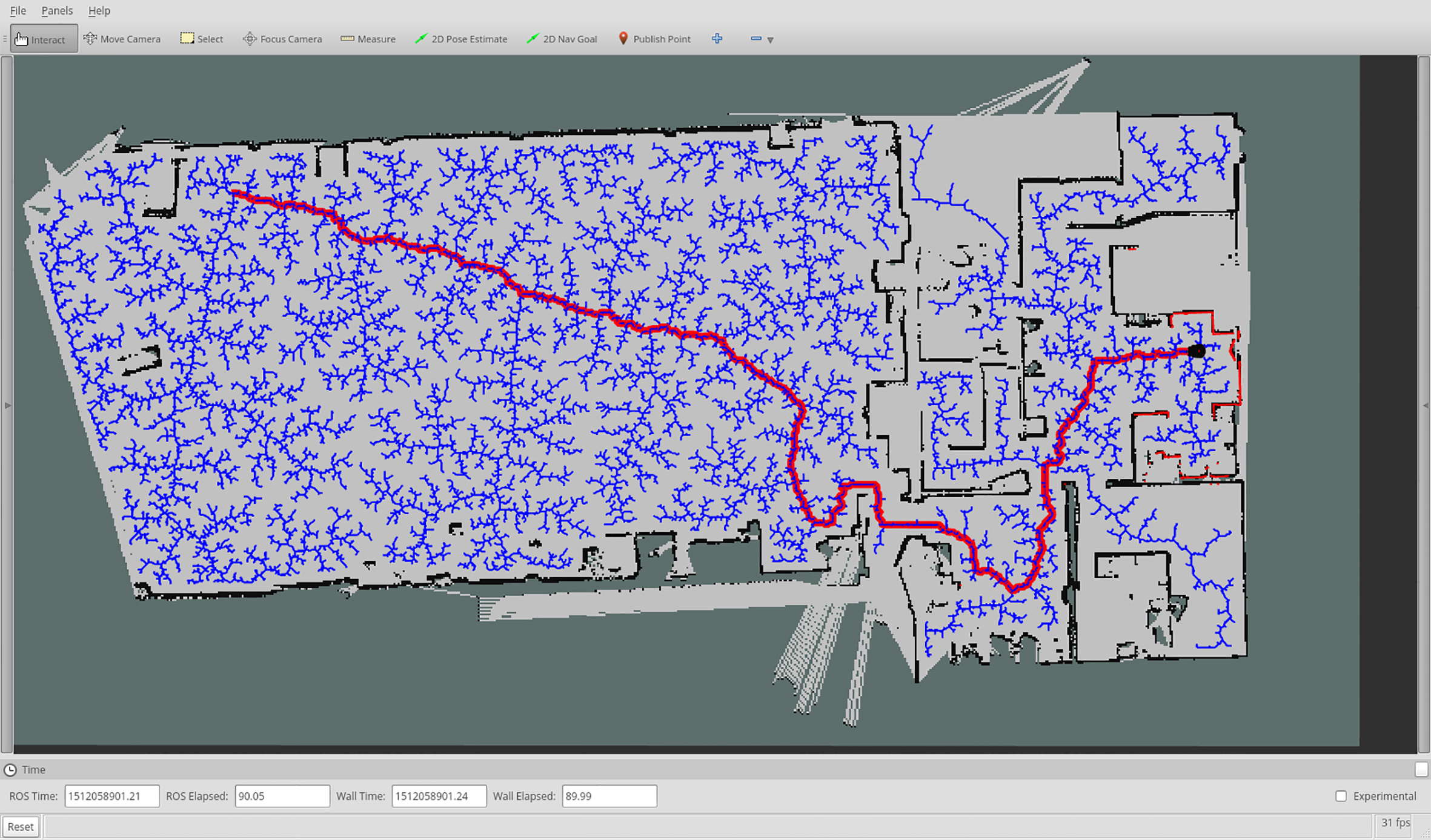
The rest of this paper is structured as follows. Next section summarizes some preliminary concepts. Section 3 is devoted to present two specific ENPS models for RRT and RRT
This section provides the reader with the basic concepts and notation used throughout this paper.
Motion planning
In general terms, the problem of motion planning can be defined in the configuration space of a mobile agent as follows. Given:
An initial configuration state. A set of valid final configuration states. A map of obstacles in the environment. A description of the agent shape. A description of the agent kinematics.
Find a sequence of configuration states through the configuration space, a.k.a. trajectory or plan, from the initial state to one of the final states, which does not touch any obstacle in the environment considering the agent shape and kinematics.
There are two variants of the problem:
The feasibility problem is to find a feasible trajectory, if one exists, and report failure otherwise.
The optimality problem is to find a feasible trajectory with minimal cost where the cost of a trajectory is given by a computable function.
In a robot navigation software architecture, the module in charge of solving the motion planning problem is called Global Planner. It computes trajectories by means of an anytime algorithm, i.e., an algorithm that can return a valid solution to the problem even if it is interrupted before it ends. After that, the Local Planner module generates motion commands to follow the trajectory in a safe manner considering the information given by the sensors in real-time. Finally, the Controller module manages the power of the actuators to fit each motion command and maintain a constant velocity until the next command, see [11].
An RRT [35] is a randomized tree structure for rapidly exploring the obstacle-free configuration space. It has successfully been used to solve nonholonomic and kinodynamic motion planning problems [36]. Nodes in an RRT represent possible reachable states, edges represent transitions between states. The root of an RRT is the initial state. Each state in an RRT can be reached by following the trajectory from the root to the corresponding node, as can be seen in Fig. 1. Algorithms used in robotics to generate RRTs are known to be anytime and any-angle, i.e., the produced trajectories could contain turns in any valid angle considering the robot constraints and kinodynamics.
The RRT algorithm
The first algorithm to generate RRTs, called the RRT algorithm [35], was able to solve the feasibility problem for motion planning in robotics.
The RRT
algorithm
The RRT
Membrane computing
P systems are theoretical computing devices biologically inspired from the structure and processes taking place in living cells [58]. As mentioned above, Membrane Computing is the field that studies these devices. The syntactic ingredients of P systems are an abstraction of chemical components and compartments of cells: a set of membranes delimiting regions where multisets of objects reside and evolve according to a set of rewriting rules. The type of membrane structure and rules depends on the class of P system, which can be cell (rooted tree), tissue (undirected graph) or neural-like (directed graph). So far, a wide variety of variants have been define within each class that answers to different semantics. In general, a computation of a P system is a sequence of configurations provided by transitions steps where the rules are executed and modify the state of the system. P systems are inherently non-deterministic and massively parallel devices, given that different sets of rules might be applicable at the same time, and each of such sets includes a high amount of rules that are executed in parallel. A global clock takes the control of each transition step.
Rules can modify only the objects in the region where they are defined, or exchange objects with a neighbor region, or modify the membrane structure by dividing or dissolving compartments, etc. Membranes can also be enriched by associating electrical charges to them. The objects that can appear in the membranes are defined in an alphabet. Several different semantics have been defined for P systems. Usually, the rules of a P system are executed in a maximally parallel way; that is, any rule that can be executed in a transition step must be executed and cannot remain unselected. On the other hand, it is possible to use a minimal parallel policy of execution; that is, at least one rule within each region must be executed. Some types of rules might be incompatible with the execution of other (e.g. division and send-out rules in active membranes), and this is given by a derivation mode.
Main research concerning P systems focuses on their computational power and efficiency, see [27, 6, 39]. In this sense, they have been used as a tool to attack the P vs NP problem by sharpening the frontiers [57, 50, 37]. However, their flexibility and massively parallelism has been employed to define modelling frameworks for real-life phenomena, such as biological systems at both micro (e.g. signally pathways, bacteria colony) [60, 23] and macro (e.g. ecosystems, population dynamics) levels [7, 14], physical systems, image processing, robot control, economic systems, etc. In general, solutions based on P systems must implement parallelism, given that this component is natural and inherent. These applications have been accompanied normally with software simulators in order to ease validation and virtual experimentation processes [16, 71]. A recent trend is to accelerate these simulations by using parallel devices like GPUs [41, 42, 13].
Numerical P systems
Numerical P systems (NPS) are P systems, see [52, 75], introduced in [59] to model economical and business processes. In NPS, the concept of multisets of objects is replaced by numerical variables that evolve from initial values by means of production functions and repartition protocols. A numerical P system is formally expressed by:
where
where
The left-hand-side of the program is called production function and the right-hand-side is called repartition protocol.
For the sake of simplicity, in the rest of this paper, we will use the next syntax:
when there is one and only one output variable in the repartition protocol.
Enzimatic numerical P systems (ENPS) are an extension of NPS introduced in [54] for modeling and simulation of membrane controllers for autonomous mobile robots. The main difference of ENPS with respect to NPS is the concept of enzyme which is used to write conditions related to programs. The formal definition of the ENPS is the following:
where
where
For the sake of simplicity, it is not necessary to write the condition function when it is the constant function
Figure 2 shows an ENPS model to generate the 100 first terms of the fibonacci succession as a toy example to illustrate how ENPS models are going to be written in this paper.
ENPS generating the fibonacci sequence.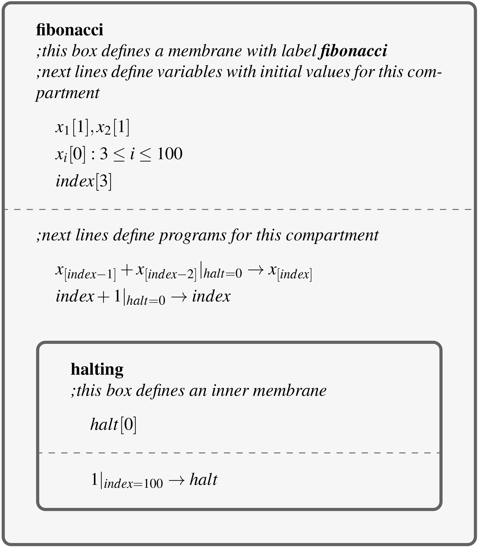
The membrane structure is designed to organize programs and variables in modules. All the variables are considered global, i.e., any program can read or write a variable regardless of the compartment where the variable is defined. The definition of variables as well as their initial values is given by the syntax
Since the advent of the transistor, computer processors have been increasing the amount of resources in order to achieve higher efficiency, and so, power [2, 65, 32]. Recent trend is to incorporate more computing cores within the same chip, so today we can easily find multicore (up to dozens of cores) and manycore (up to thousands of cores) processors in the market [3, 53]. The former concerns current CPUs, and the latter involves mainly GPUs. The main standard to harness the parallelism in multicore processors is OpenMP [49], which is managed by the OpenMP ARB consortium. First introduced in the late 90’s, it provides an API for common languages such as Fortran, C and C
Nowadays, GPUs can be used as manycore processors to accelerate scientific computation [31, 18]. CUDA [47] is the most widely used programming model, given that it was first introduced in 2007 by NVIDIA, and it has been strongly supported by this company. Although OpenCL is the standard introduced by Kronos for GPU computing, CUDA is still better supported by NVIDIA GPUs. In any case, similar concepts can be found in OpenCL and in CUDA. It is a heterogeneous programming model where CPU (host) and GPU (device) are separated, and so, has different memory spaces. GPUs contain several multiprocessors including computing units and fast shared memory system, and all multiprocessors are interconnected with a global memory that can be also accessed by the CPU, specially to copy and retrieve data. CUDA provides an abstraction of the GPU in form of threads that execute the same code which is a function called kernel [45]. Threads are grouped in blocks, so each block is assigned to a multiprocessor, being able to efficiently cooperate locally inside the blocks. CUDA programmers have to manage these aspects manually: thread grid and memory layout. Moreover, threads are executed completely in parallel when they are fully synchronized in the code; that is, they follow a SIMD fashion (single instruction multiple data). Moreover, accesses to memory get optimized when threads query contiguous positions of data [45, 51]. Therefore, parallel algorithms have to be carefully adapted to this model bearing in mind several efficiency aspects. Some algorithms fit very well to the GPU architecture and so they are employed as primitives and building blocks, such as map (application of a function to all elements of a vector), reduction [33] (calculation of a function over all elements of a vector), scan (accumulative application of a function to elements of a vector), etc. [31, 51].
ENPS models for RRT algorithms
In this section, four ENPS models are presented in order to simulate the behavior of the RRT and RRT
Find the nearest point to a given point according to the Euclidean distance. Determine if a given trajectory is obstacle free. Simulate the RRT algorithm. Simulate the RRT
The main ideas of the P system design are the following:
To use enzymes in order to synchronize the processes. To compute Euclidean distances in parallel. To use a parallel reduction process in order to compute minimum distances. To add a node to the RRT in each iteration.
Given a set of points
Solution for
3
The solution of the nearest point for
Nearest(3) procedure.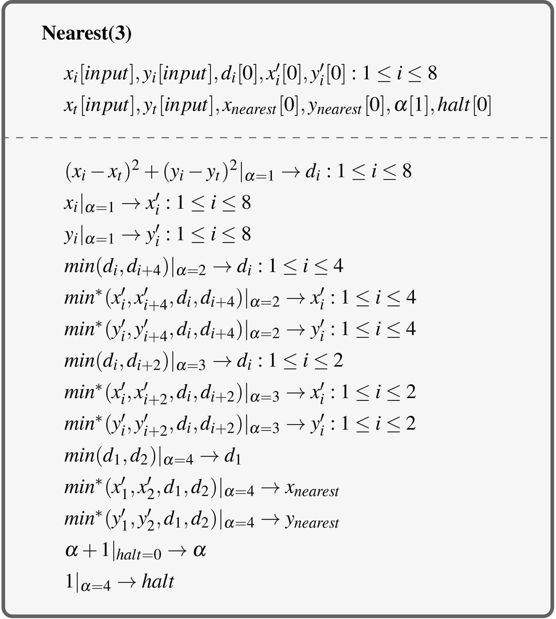
General Nearest(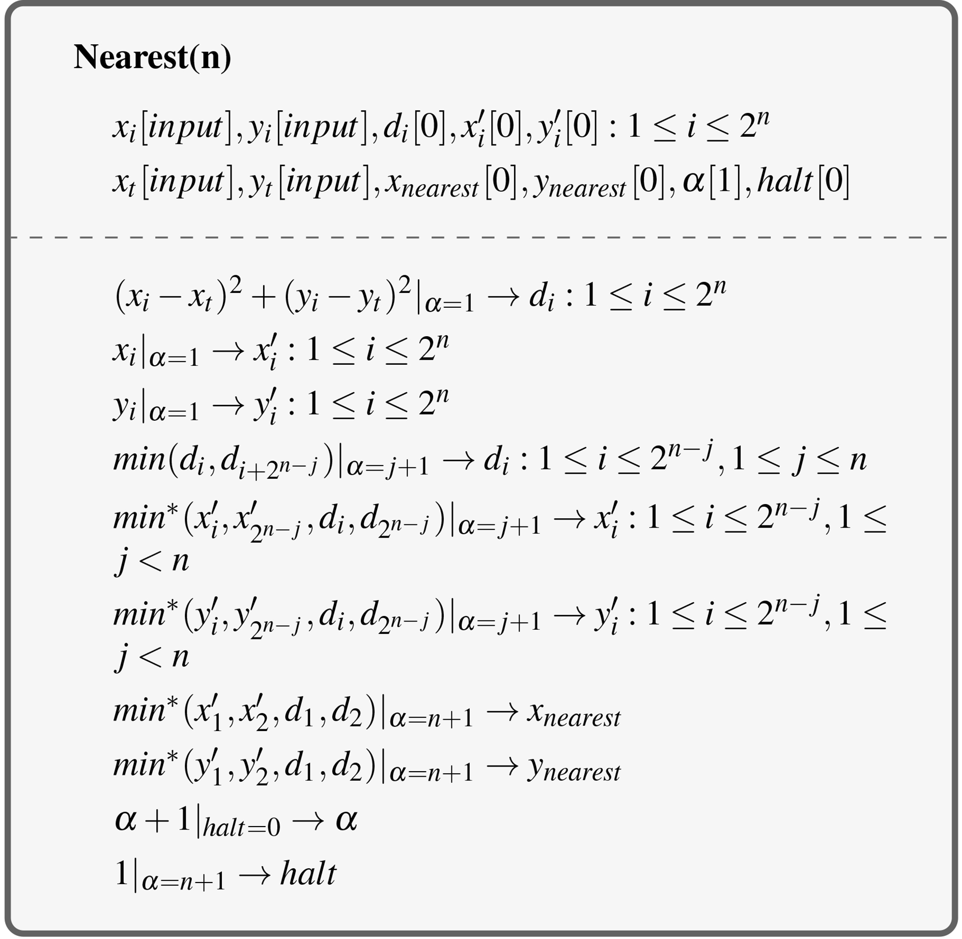
The P system computes in one step of computation the squared Euclidean distance for all the points in
The general solution, for
After
Obstacle free trajectories
Given a set of obstacle points
Procedure for the detection of an obstacle free trajectory.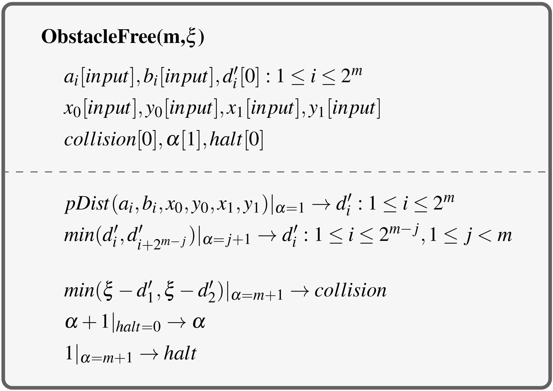
With reference to Fig. 5:
After
Algorithm 1 shows the pseudocode of the pDist function.
The P system computes in one step of computation the squared Euclidean distance for all the obstacles to the segment given by
For the following set of parameters
An initial robot position A set of obstacle points The size Parameter Parameter Parameter
the RRT algorithm is illustrated in Fig. 6.
Rapidly-exploring random tree.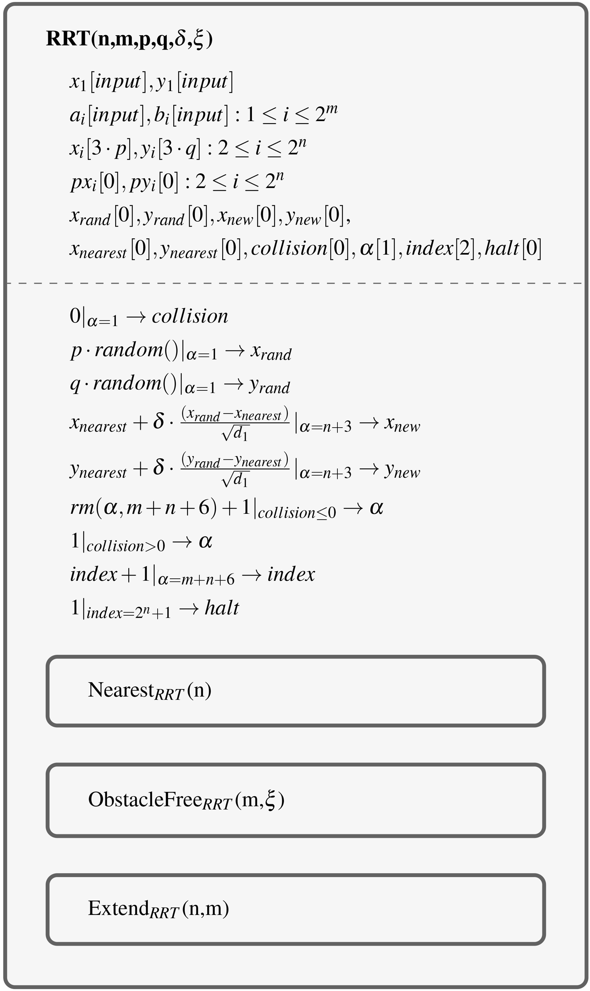
The inner modules are defined as shown in Figs 7–9 where
The coordinates of the RRT nodes will be The coordinates of the RRT parent nodes will be The RRT is completely generated and the computation stops when
Nearest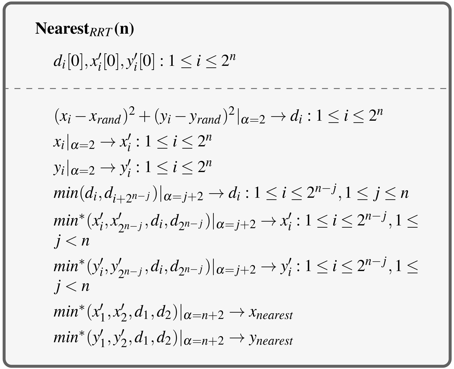
ObstacleFree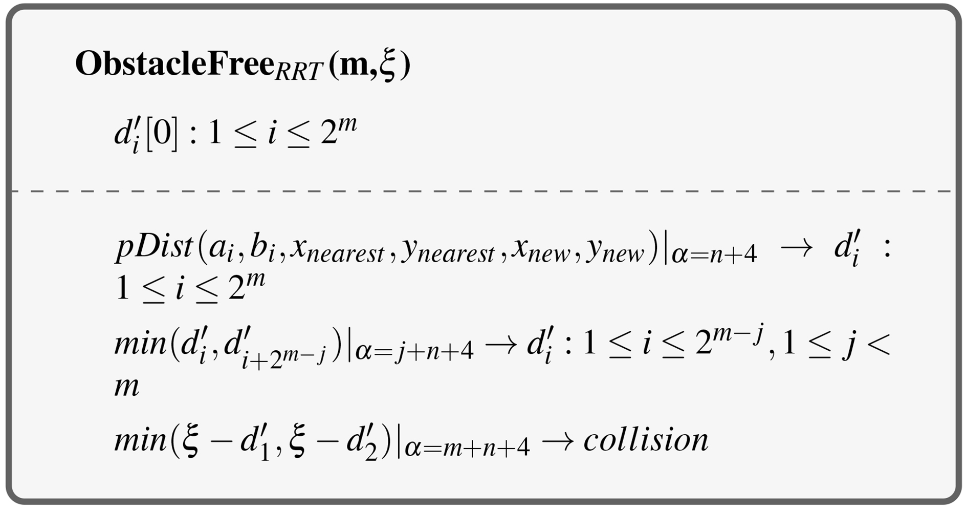
Extend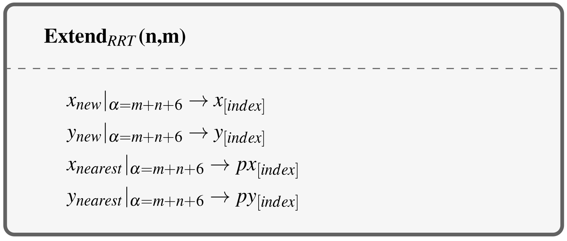
The P system generates the point
The asymptotically-optimal version of the RRT algorithm, i.e. the RRT
Asymptotically optimal Rapidly-exploring Random Tree (RRT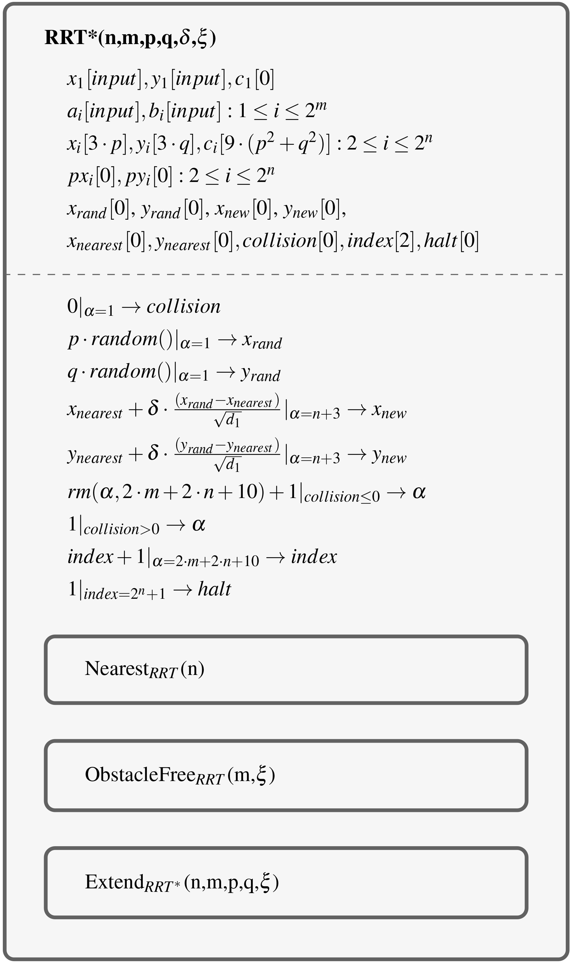
Extend
The first
We have implemented two specific (ad-hoc) simulators using OpenMP and CUDA, each one is able to simulate the ENPS-RRT and ENPS-RRT
The conventional RRT and RRT
An OpenMP simulator
The OpenMP simulator is able to manage image files in PGM format defining the obstacle maps, four predefined scenarios have been included with the software as it will be explained in Section 5. For each one, a PGM file is included along with a fixed initial position for the robot. The resolution for all maps is 5 cm
The software provides a command-line interface in order to specify the scenario to be used, as well as the model (ENPS-RRT or ENPS-RRT
The software allows to set all the parameter values. For the experiments in this paper, the next set of values has been used:
The selected values for
The simulator uses data structures to store the value of the ENPS variables in run-time and programming sentences in C with OpenMP in order to simulate the behaviour of the ENPS programs. That is, the simulator allocates arrays storing the objects for:
obstacle positions ( RRT points and their parents, ( auxiliary objects for reduction at nearest (
Moreover, the simulator is written in a modular way, where it is easy to identify the different modules of the model:
Computing (
nearest, in order to compute (
computing squared distances from all points in RRT to ( computing minimum distance and nearest point in RRT
obstacleFree, in order to compute obstacle collision. This is done by:
compute distances from all obstacles to segment [( Compute minimun distance to check if there is collision, by comparing with the epsilon variable
Extend RRT, if using RRT algorithm.
Extend RRT
computing squared distances from all obstacles to all segments [( for each point ( compute new cost for all points in RRT compute the minimum cost and the variable with that value (that is, argmin operation) fix the edges in RRT
As an example, the next C/OpenMP code computes the squared distances from all the points in the RRT to the
In order to compute minimums in a whole array, we can use reduction pattern. That is, calculate a value from a whole collection, in this case, a minimum. Reduction is implemented in OpenMP by a special directive extension [17]. For instance, the next code shows the computation of the minimum distance and nearest point:
Additionally, we have outsourced the ad-hoc simulator to the GPU. This enables its parallelization for both high-end and low-end GPUs by using CUDA. Let us recall that this technology provides automatic scalability and portability of the code. Thus, the most computing-intensive part of the simulation is executed on device, what will allow to accelerate its execution significantly, as we will discuss in the results. First of all, we have replicated the data structures employed on the OpenMP simulator on the GPU.
Simple map functions applied to objects in parallel are implemented by CUDA kernels, optimized by launching 256 threads per block (we have tuned this number experimentally), a number of thread blocks multiple of the amount of streaming multiprocessors on the specific device, and looping by tiles over the objects (contiguous threads work with contiguous positions of arrays, and iterate in this manner until covering all positions). The following parts are implemented in this way:
At nearest module, computing squared distances from all points in RRT to ( At obstacleFree module, computing the distances from all obstacles to segment At RRT
computing squared distances, using pDist, from all obstacles to all segments computing new cost for all points in RRT, while checking the minimun distance is greater than epsilon. Fixing edges.
As made for the OpenMP implementations, global minimum calculations can be efficiently implemented by the reduction operation. In CUDA, reduction is a parallel primitive, and there is a plethora of optimized implementations. We have focused only on reduction with minimum operation for floating numbers. We have tested three different libraries in order to select the fastest one: (1) reduction example from CUDA Toolkit SDK 10.1 [47], (2) Thrust (as redistributed in CUDA 10.1) [26], and (3) CUB 1.8 [43]. Implementation (1) is based on the optimization ideas using per-warp shuffle operations [38], available first in Kepler architecture. We have modified the implementation in the SDK by replacing the sum (
We have therefore used CUB to compute the following reduction operations:
At nearest module: compute minimum distance and nearest point by using argmin reduction. At obstacleFree module: compute minimum distance by using min reduction. At RRT
Compute the minimum distance for each point (x,y) in RRT to all obstacles. This requires to construct a matrix with a row per RRT point and columns the number of obstacles. We have used the segmented reduction minimum variant to calculate all the minimums per row in parallel. This variant performs reduction globally but it only takes effect inside local segments that are previously defined. Compute minimum cost by argmin.
Finally, in order to keep all the computation on the GPU and hence, avoiding transferring data from the GPU to the CPU at every iteration, store also the scalar values of
In this section, we will show the experiments conducted to test the performance of the ad-hoc simulators for both OpenMP and CUDA. We first start analyzing the results for the multicore version, selecting the best configuration. After that, we show the runtimes obtained with GPU version, and conclude with a comparison of configurations.
The source code of the simulators is written in C/C
Speedup using OpenMP for different multithreading configurations with respect to the sequential implementation for each baseline algorithm and for each map
Maps employed in the experiments. Maps are sorted by complexity: (a) is map1 (a simple room), (b) is ccia_h (scanned map of the computer science department’s wing H at University of Seville), (c) is office (a set of rooms in an office), and (d) is maze (a labyrinth composed of concentric circles).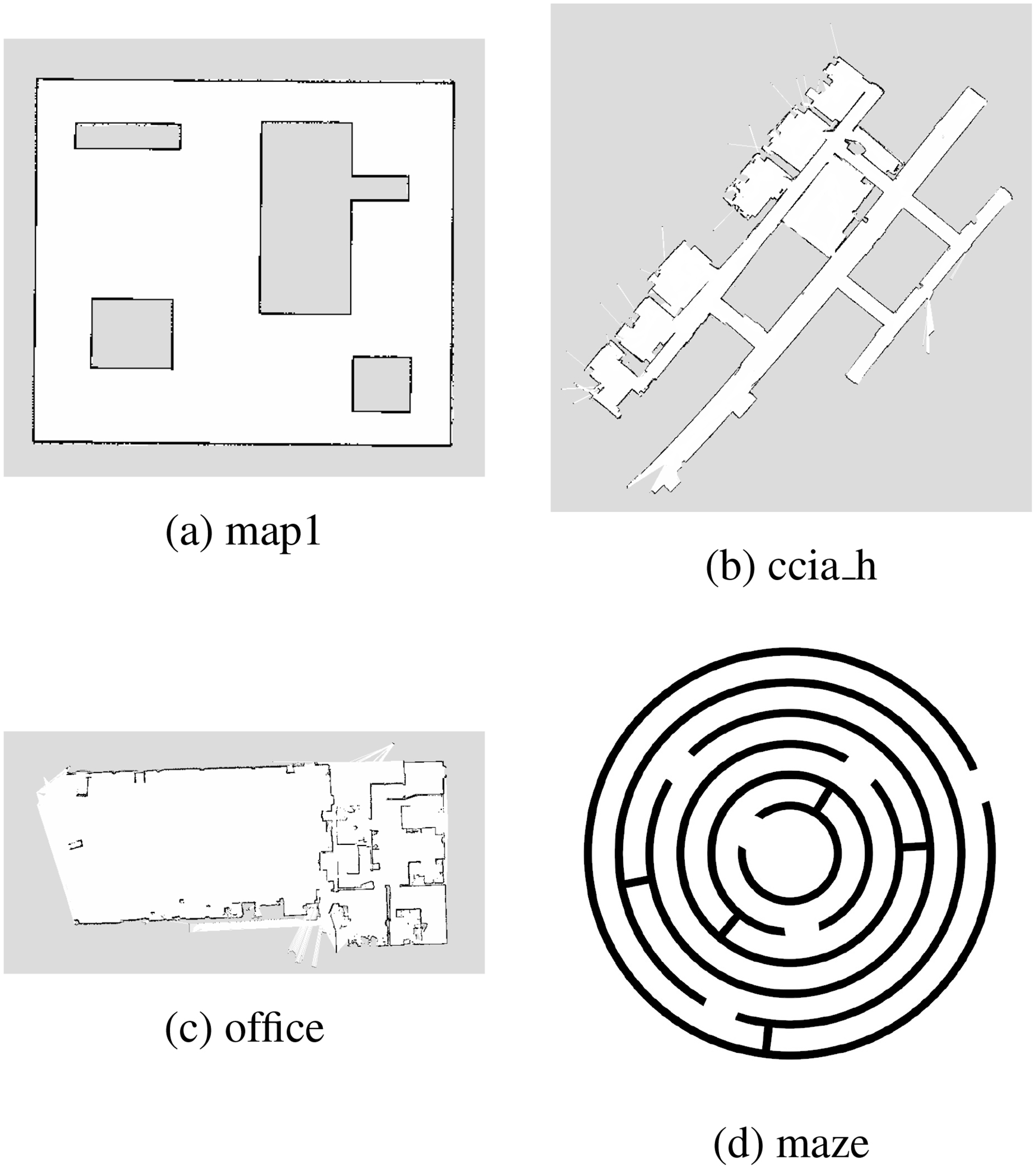
Runtimes of the OpenMP simulator for RRT on the i7-8700 (a) and i7-9700 (b) CPU. X-axis shows the number of cores used during execution (1 to 12 for i7-8700, and 1 to 8 for i7-9700, both by step of 2). Y-axis shows the time in seconds.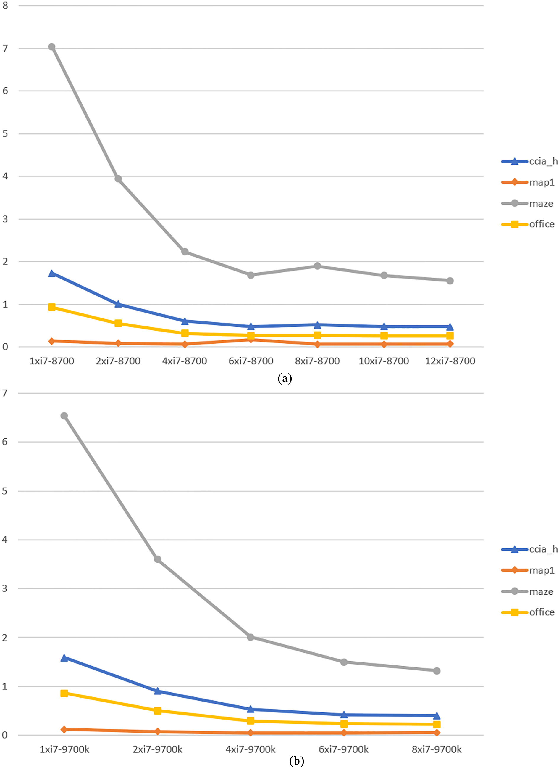
Runtimes of the OpenMP simulator for RRT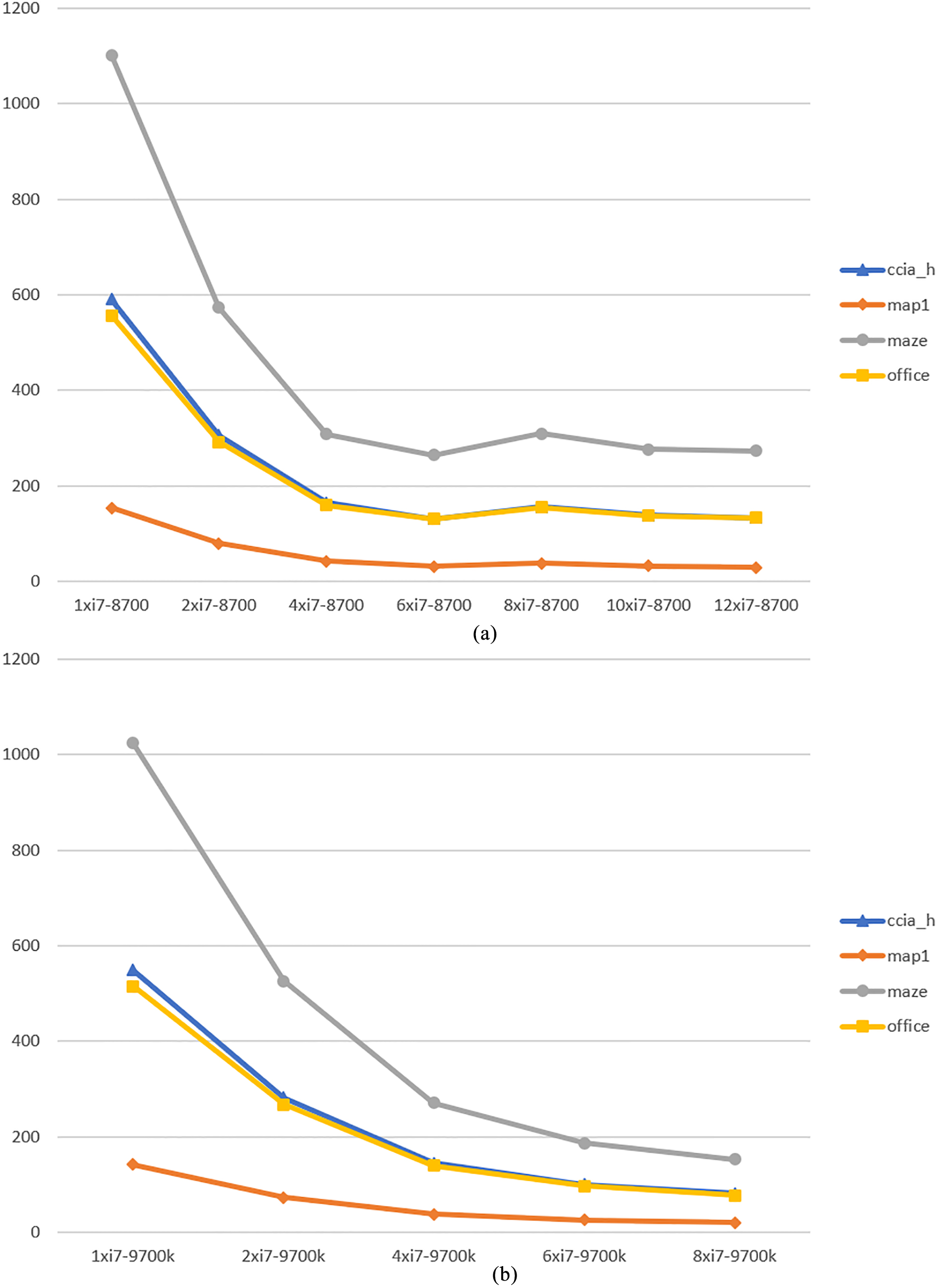
Runtime of the CUDA simulator for RRT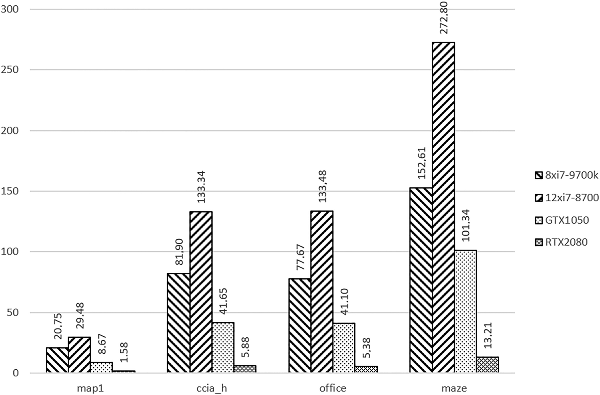
Seedups obtained comparing the best and worst configurations for both CPU and GPU.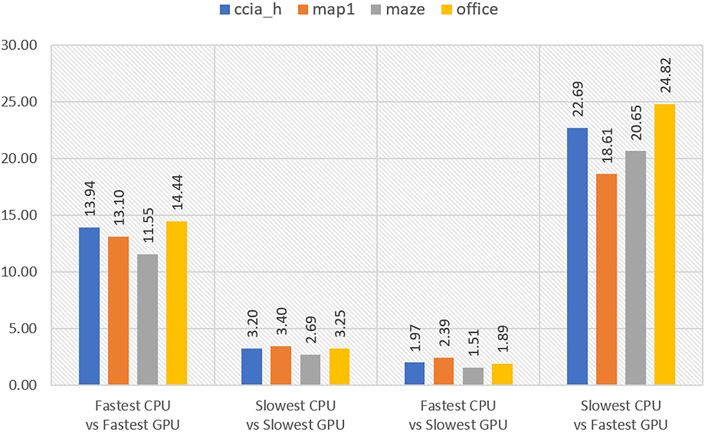
We have used four different maps for the experiments. These are shown in Fig. 12. We have sorted them by increasing complexity, so that we expect that RRT and RRT
In Fig. 13, the runtimes of the multicore simulator for RRT are displayed. We increase the number of threads by 2, starting in 1 and until the total amount of cores in the corresponding CPU. We can see how it scales well and the runtime drops proportionally to the number of threads executed, specially when going from just 1 thread to the half amount of cores in each CPU. Runtimes from half to all cores remain almost constant. Only in maze we can experiment some improvement. Low-complexity map1 is handled fast in all CPUs, so running several threads is not worthy. Finally, runtimes are similar in both CPUs, and is always below 2 seconds when using all cores. For i7-8700, a speedup from 1.8x (map1) to 4.5x (maze) is obtained when using all cores against just one core (sequential version). For i7-9700, a speedup from 2.2x (map1) to 4.9x (maze) is achieved.
We can see some differences when running the multicore simulator with RRT*, given its higher complexity. The runtimes are plotted in Fig. 14. For i7-8700, half of the cores (6) are enough to saturate the processor. For i7-9700, the best runtime is achieved with full occupancy of the cores (8). We can see how the runtime decrease is proportional to the amount of cores again. Runtime for i7-9700 is slightly lower than for i7-8700, being below 200 seconds against 300 seconds in the latter. The map maze requires the higher computation time. For i7-8700, a speedup from 4x (maze) to 5.2x (map1) can be obtained when using all cores against the sequential version. For i7-9700, a speedup of around 6.7x for all maps is reported.
In Fig. 15, we compare the runtimes obtained with the GPU against the CPU. We consider for this experiment the best configuration for both CPUs, that is using all the cores in each processor. For RRT
Finally, let us assume the best and worst device: fastest CPU is i7-9700 with 8 cores, slowest CPU is i7-8700 with 12 cores, fastest GPU is RTX2080 and slowest GPU is GTX1050. In Fig. 16, we show the speedups obtained by comparing one by one the devices tested for RRT
In light of the results, we can draw the following conclusions: CPU is the best candidate if we want to run the adhoc simulator for RRT, and the GPU is always the best candidate to run the ad-hoc simulator for RRT
In this work we present two ENPS models emulating the computation of the RRT and RRT
Footnotes
Acknowledgments
This work is supported by the research project TIN2017-89842-P (MABICAP), co-financed by Ministerio de Economía, Industria y Competitividad (MINECO) of Spain, through the Agencia Estatal de Investigación (AEI), and by Fondo Europeo de Desarrollo Regional (FEDER) of the European Union. This work is supported by the National Natural Science Foundation of China (61972324, 61672437, 61702428), and also funded by Beijing Advanced Innovation Center for Intelligent Robots and Systems (2019IRS14), Artificial Intelligence Key Laboratory of Sichuan Province (2019RYJ06), the New Generation Artificial Intelligence Science and Technology Major Project of Sichuan Province (2018GZDZX0043) and the Sichuan Science and Technology Program (2018GZ0185, 2018GZ0086).