Pattern discovery in time series using autoencoder in comparison to nonlearning approaches

Abstract

In technical systems the analysis of similar situations is a promising technique to gain information about the system’s state, its health or wearing. Very often, situations cannot be defined but need to be discovered as recurrent patterns within time series data of the system under consideration. This paper addresses the assessment of different approaches to discover frequent variable-length patterns in time series. Because of the success of artificial neural networks (NN) in various research fields, a special issue of this work is the applicability of NNs to the problem of pattern discovery in time series. Therefore we applied and adapted a Convolutional Autoencoder and compared it to classical nonlearning approaches based on Dynamic Time Warping, based on time series discretization as well as based on the Matrix Profile. These nonlearning approaches have also been adapted, to fulfill our requirements like the discovery of potentially time scaled patterns from noisy time series. We showed the performance (quality, computing time, effort of parametrization) of those approaches in an extensive test with synthetic data sets. Additionally the transferability to other data sets is tested by using real life vehicle data. We demonstrated the ability of Convolutional Autoencoders to discover patterns in an unsupervised way. Furthermore the tests showed, that the Autoencoder is able to discover patterns with a similar quality like classical nonlearning approaches.

Keywords

Time series data mining pattern discovery motif discovery autoencoder unsupervised

1. Introduction

A pattern is informally defined as recurring similar subsequences within a time series. As the focus of this work is unsupervised pattern discovery, the patterns are unknown in advance. Depending on the background of the user the intuition of a pattern can vary a lot and therefore lead to misunderstandings. One of the most used names in the wide field of pattern discovery in time series is motif discovery. Unfortunately definitions of motifs are not consistent in the literature. For example within the Matrix Profile approach it is defined as “the most similar subsequence pair of a time series” [1]. while Lin et al. described it as “a pattern that consists of two or more similar subsequences based on some distance threshold” [2]. To solve this inconsistency this work assumes a motif to be defined as a query subsequence and the subsequence that is most similar to the query, while the task of motif discovery is to find the best (most similar) motifs. Hence, a motif always only consists of two subsequences. In contrast to this a pattern is a group of $\geqslant$ 2 similar subsequences in a time series.

In general, we need reliable methods to detect recurring patterns with variable and previously unknown length in noisy time series. A pattern and its members should be similar in shape and invariant regarding offset and amplitude. Beyond this, we allow members of a pattern to be scaled in time to a certain amount. Suitable approaches need to be able to process data sets with far more than one million data samples at a reasonable runtime. Furthermore we also need to detect patterns in multivariate time series. However, in this paper we limit our analysis for simplicity to the univariate case. Following these requirements we will compare four different approaches from different research areas. First of all, the focus of this work is the investigation and development of an approach for pattern discovery based on artificial neural networks (NN). As a reference three nonlearning2 approaches will be implemented, that have already been proposed in previous work of [3].

1.1 Motivation

The analysis of time series data recorded from the operation of complex mechatronic systems provides information on usage, condition or even misbehavior of systems or components. In order to obtain long-term information on these objectives an analysis of the entire data record is required. In the context of wear-off or aging of systems having recurring load patterns it is advantageous to compare only such patterns. In our use case, we cannot expect experts to specify suitable patterns and therefore we need unsupervised methods for automatic definition of such recurring stress patterns without input of expert knowledge. The previously listed requirements for an unsupervised pattern discovery method are derived from these use cases.

In recent years the research in NNs succeeded in many disciplines. Rodríguez Lera et al. [4] for example, proposed a feedforward NN to recognize human activities in “at home” scenarios. In [5] Lara-Benítez et al. developed a deep learning framework for streaming data classification. A convolutional NN was applied by Molina-Cabello et al. in [6] in order to detect differenent kinds of vehicles based on video data. Macias-Garcia et al. [7] even applied two NNs in parallel to seperately detect obstacles and targets for mobile robots. Due to the great variety of applications it is evident to evaluate the possibility to apply NNs to the problem of unsupervised pattern discovery, too. While there are existing nonlearning approaches for our requirements, the amount of approaches based on NNs is nearly not existing. In this work we want to investigate the possibility to discover interpretable patterns based on NNs and rank them regarding nonlearning approaches.

1.2 Related work

In general NNs can be applied as supervised or unsupervised learning techniques. In the case of supervised use cases, like classification tasks, a great variety of NNs has already been developed to enhance classical feedforward NNs. In [8] for example, the authors proposed a more robust and dynamic approach for the optimization of their NN-based classifier and compared it to an enhanced probabilistic NN, which contains Bayesian rules and is said to be simpler and more efficient [9]. In [10] the authors even used an ensemble of NNs and proposed a technique to automatically design the ensemble. For the sake of completeness, there are also modern learning techniques that are not based on NNs. For example in [11] the authors proposed a finite element machine classifier for supervised learning problems. Even though these learning techniques are very interesting for the supervised case, they are not explicitly made for the unsupervised case of finding patterns without their prior knowledge.

The basic idea of the NN-based approach relies on the unsupervised feature-learning in time series data, while these features should represent or correlate with the patterns that need to be identified. In general [12] gives a good overview of techniques concerning the unsupervised feature learning in time series, but it does not focus on the extraction of sequential patterns, like it is necessary for our use cases. Instead, the interpretability of these features is mostly difficult, which is not a problem for e.g. classification tasks. In [13, 14] the authors proposed unsupervised feature learning techniques to identify shapelets, which are maximally discriminative features of time series. In [15] shapelets are defined as “subsequences which are in some sense maximally representative of a class”. Unfortunately this definition does not totally match with the definition of a pattern. A technique that is closely related to our pattern discovery problem is Convolutional Autoencoding. By the use of fully convolutional layers in NNs it is possible to extract e.g important and recurring parts of images. In [16] Benamara et al. for example applied convolutional NNs to extract human emotions based on facial images. Autoencoders like in [17, 18, 19] are able to learn important features of the input data by first encoding the input data to a lower dimensional space and then decoding it to reconstruct the input. While the unsupervised extraction of patterns from image or video data is a common task for Convolutional Autoencoders (CAE), the pattern discovery in time series is an underrepresented problem. In the following sections we take up some ideas regarding the architecture of CAEs from [17] and complement them by multiple additional methods to detect recurring patterns in time series data.

The first nonlearning reference approach is based on the principle of dynamic time warping (DTW). DTW is a distance or similarity measurement for time series with different lengths with the possibility to stretch or compress one of the time series to fit the other one [20]. Beyond that, DTW can be adjusted and extended to the problem of discovering patterns. The authors of [21] proposed a DTW-based algorithm called CrossMatch to identify similar subsequences in different sequences without the need of a query sequences. A similar technique is described in [22] where the approach is extended by a hierarchical clustering algorithm to find patterns.

The second type of approach is based on the symbolic representation of the time series, which is interesting in terms of reduction of complexity and therefore also for the reduction of runtime. However, these approaches can be more sensitive against noise than those based on DTW. To get a symbolic representation, there are many methods for time series discretization. The Symbolic Aggregate Approximation algorithm (SAX) [23] and other symbolic time series methods use intervals with equal probability. Besides, there is the possibility to use intervals of equal size. The relevance of symbolic approaches is evidenced by the variety of existing pattern discovery algorithms from various research fields like bioinformatics or text mining. For example in bioinformatics the Smith Waterman algorithm is used for sequence alignment, meaning the pattern discovery in DNA sequences [24]. As DTW, Smith Waterman is based on dynamical programming and is able to find time scaled patterns. The Sequitur algorithm, proposed in [25], extracts the hierarchical structure of a symbolic sequence by replacing recurring phrases with grammatical rules while forming a dictionary of these rules, which is formally known as grammar induction. Sequitur identifies only identical patterns and ignores possible similarities in rules/patterns. Furthermore it is not guaranteed to find all the patterns in the sequence, because of its replacing procedure. Pattern enumeration is often referenced to cope with this problem. To perform time scaled pattern discovery with those algorithms numerosity reduction techniques have been proposed, as e.g. employed in [2]. Especially for long sequences the number of enumerated patterns can increase exponentially. That is why there is also research in constraint programming techniques like in [26] or [27]. Beyond these methods, there is a huge amount of algorithms regarding pattern mining in symbolic sequential data summarized in [28].

The third approach is the Matrix Profile introduced by Keogh, Mueen, Yeh and Zhu [29]. Basically, it is a brute force approach to find motifs or patterns of a fixed length by calculating the distances between every possible query sequences and every other sequence of the chosen length. Nevertheless, since the Matrix Profile I was published in 2016 it grew to an open source framework for many time series analysis task. Until today the authors published more than 20 papers regarding the optimization, extension and application of Matrix Profile, which are consecutively named as Matrix Profile I to XX [29, 30]. Unfortunately all these publications focus on using the z-normalized Euclidean distance as a distance measure. Hence, it only allows e.g. patterns to be similar just in shape and ignoring the offset or amplitudinal scaling. Beside that, longitudinal scaling is not supported. A possibility to solve these issues is to replace the z-normalized Euclidean distance by DTW. However, all those optimizations proposed in the Matrix Profile framework [31, 32, 33] are based on z-normalized Euclidean distance, which is why the computational intensity would be to high to be competitive. Beyond that, this theoretical solution still does not solve the problem of fixed length pattern discovery. In Matrix Profile X [34] and XX [30] the authors additionally proposed solutions to this problem, but again focused on z-normalized Euclidean distance. Due to the fact, that Matrix Profile is still a relevant approach, we implemented an optimized version of the standard Euclidean distance as a reference to other approaches.

1.3 Purpose and structure

First of all, this work will demonstrate the ability of NNs to discover unknown patterns. The architecture and techniques that are crutial in order to guarantee the functionality will be proposed and critically evaluated. Furthermore, this paper deals with the comparison of the NN-based approach regarding aforementioned nonlearning approaches. Our target is an evaluation concerning runtime, parameterization effort and pattern quality. Therefore we apply different quality measures, which gives us the opportunity to evaluate and compare different approaches.

The remainder of this work is organized as followed: In Section 2 an NN-based approach using CAE is proposed for the unsupervised discovery of patterns. Section 3 deals with nonlearning approaches, which were already been proposed in previous work [3] and are now considered as relevant references for the NN-based approach. Section 4 explains the approach for the comparison of pattern discovery algorithms equivalent to previous work [3]. Section 5 evaluates the results and gives statements concerning the assessment of different approaches. After discussing the developments and findings of this work in Section 6, Section 7 finally gives a conclusion and an outlook to future research regarding pattern discovery with unsupervised feature learning techniques.

2. NN-based approach for pattern discovery

There are many techniques for unsupervised feature learning in time series. Unfortunately most of these learned features lack in terms of interpretability. To solve this issue we chose a Convolutional Autoencoder (CAE) for further investigations. The idea is to reconstruct the input time series with convolutional encoding and decoding filters, while the filters contain interpretable features of the input time series. These features will represent the patterns that are contained in the input time series and which are necessary to reconstruct it. As we will show in the next sections by the use of 2D convolution, it is possible to interpret the extracted features as patterns in the common sense.

2.1 Convolutional autoencoder

We take up basic ideas of CAE architecture of [17]. It contains a convolutional and a sparsity layer, which are used for encoding the input images in a lower dimensional space. A deconvolutional layer then decodes the output of the sparsity layer to the input space. The convolutional and the deconvolutional layers consist of an equal number of filters, whereas one filter represents a pattern, which is necessary to reconstruct the input image. This network is trained by gradient descent method with the input being the desired output.

The approach of [17] offers the possibility to autoencode time series by 1D-convolution or images by 2D-convolution. We experienced that this architecture is rather optimized for autocoding of images instead of time series. In fact, we were not able to produce any kind of promising result with 1D-convolution. Due to more promising image autoencoding we decided to merge the advantages of 2D-convolution with time series analysis by creating a new 2D-representation of time series. In the end, this decision turned our to be the biggest enabler for NN-based unsupervised pattern discovery.

The time series is converted to a grey-scale image in two steps. First the time series is discretized with a given number of bins, as described in Section 3.2 of the discretization-based reference approach. Then the discretized time series is converted to an image by one-hot-encoding as shown for a small subsequence in Fig. 1. One major difference between a regular image and a time series image is its size. While a dataset of regular images always contains images of the same dimension, our time series dataset is just one very wide time series image. Hence, to fit this time series image in CAE we cut it in slices with an equal width.

Figure 1.

Conversion of a discretized time series to an image; right: discretized time series; left: one-hot-encoded image.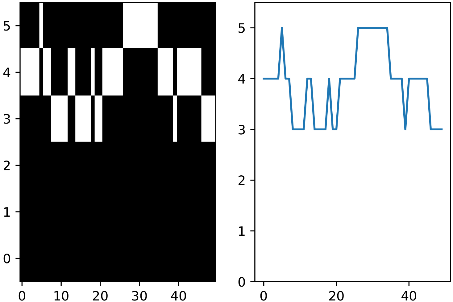

Figure 2.

Exemplary input, filter, latent space and output of the Autoencoder for time series.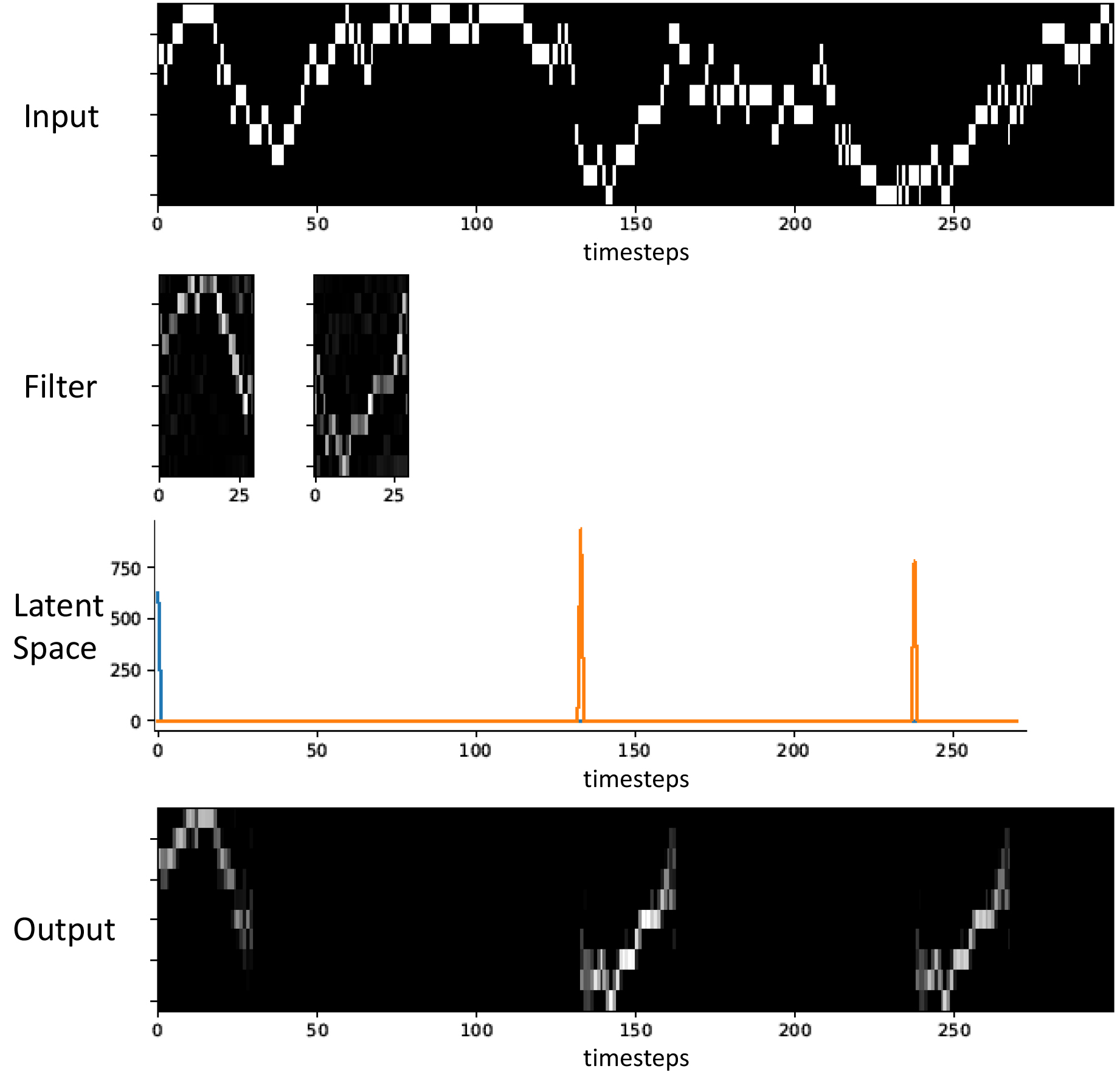

Figure 3.

Left: good fit of a pattern; right: bad fit with noise.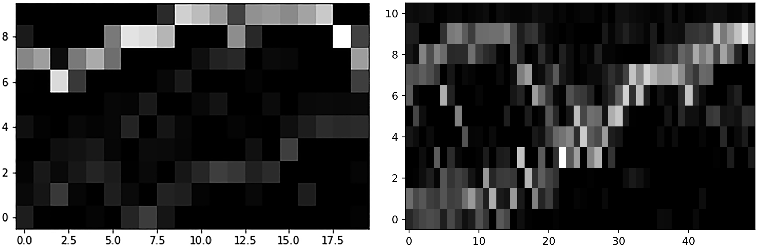

Assuming we already have a pretrained CAE, a convolutional filter contains an one-hot-encoded representative subsequence of a pattern, which is exemplarily shown for two patterns in the second row of Fig. 2. In the forward path through CAE, the convolutional layer at first produces one latent space vector per filter, which can be interpreted as a similarity vector of the convolutional filter and the corresponding subsequences of the input. Within the sparsity layer, the latent space vector is filtered, by setting every value to zero, except for the peaks. Therefore the parameter latent limit sets a relative threshold for these peaks. In the example of Fig. 2 the third row shows these filtered latent space vectors of both convolutional filters. The peaks are referring to the starting indices of similar sections in the input image. Hence, the deconvolutional layer can reconstruct at least parts of the input with these two filters and the latent space vectors.

In [17] the authors proposed additional regularization terms to enable CAE to identify patterns in images. Unfortunately not all of them are working for the case of a time series and the identification of recurring subsequences. We need the filters to represent a subsequence as clear as possible, which implies that in one column only very few pixels should be highlighted. While testing CAE of [17] we also discovered some artifacts, e.g. one filter containing two different patterns. An example for a good and a bad fit of a convolutional filter is shown in Fig. 3. To push CAE into optimizing the filters, we propose adaptions of the original CAE in the next subsection.

2.2 L1 regularization

The $l_{1}$ regularization was already proposed in [17] and is also helpful in our use case. In general the term helps keeping the weights low, which at the same time keeps the number of highlighted pixels in the filters down. It is defined as:

$\displaystyle l_{1}=\sum_{n=1}^{nf}\sum_{i=1}^{h}\sum_{j=1}^{fl}|w(n,i,j)|$ (1)

with $n f$ : number of filters; $h$ : height of filter; $f l$ : length of filter; $|w(n,i,j)|$ : absolute value of weight in $n^{\text{th}}$ filter at the position ( $i, j$ ).

Hence, the variable $l_{1}$ represents the sum of all weights of all convolutional filters. By adding $l_{1}$ to the cost function, the Autoencoder will try to minimize the overall weight of all filters. Furthermore the quantifier $\lambda_{L}$ is introduced to control the influence of the $l_{1}$ regularization in the cost function. One of the previously described requirements for pattern discovery algorithms is the identification of variable-length patterns. But until now it is only possible to identify patterns of fixed length with CAE, because of the given filter length. To solve this issue we propose for simplicity the application of multiple CAEs with varying filter lengths, while the filter length within one CAE is constant. According to this, we added parameters for the minimum and the maximum filter length, as well as $\Delta fl$ for the evaluation in Section 4.2. $\Delta fl$ defines the difference in the filter length from one CAE run to the next. By summarizing the results of each run, a global result for the variable length pattern discovery is produced.

As described in Eq. (1), the size of $l_{1}$ strongly depends on the number of weights, which again depends on the number, height and length of the filters. When varying the length of the filters, it is therefore also necessary to dynamically adapt the value of $\lambda_{L}$ to keep the influence of $l_{1}$ on a constant level. In the next sections more terms will be added to the cost function. These terms are not dependent on the number of weights, which is why the influence of $l_{1}$ would increase with growing filter lengths. Hence, we propose to replace the parameter $\lambda_{L}$ by a term, which dynamically adapts to the number of weights:

$\displaystyle\text{NW}=nf\cdot h\cdot$ (2) $\displaystyle\lambda_{L,dyn}=\lambda_{L}\cdot\text{NW}$ (3) $\displaystyle\lambda_{L}=\frac{\lambda_{L,dyn}}{\text{NW}}$ (4)

with NW: total number of weights; $\lambda_{L,dyn}$ : parameter for influence of $l_{1}$ regularization.

2.3 Entropy

The idea of using entropy for the optimization was already applied at [17]. The author’s goal was to minimize the entropy in the latent space vector to have only few and high peaks in the vector. Hence, it has a similar impact compared to the sparsity layer. We transformed the concept into an entropy at the level of convolutional filters and their pixels:

$\displaystyle\textit{ENT}=-\sum_{n=1}^{nf}\sum_{i=1}^{h}\sum_{j=1}^{fl}p(n,i,j% )\cdot\log{p(n,i,j)}$ (5)

with

$\displaystyle p(n,i,j)=\frac{w(n,i,j)}{\sum_{\hat{n}=1}^{nf}\sum_{\hat{i}=1}^{% h}\sum_{\hat{j}=1}^{fl}w(\hat{n},\hat{i},\hat{j})}$ (6)

with $|p(n,i,j)$ : probability of weight $w$ in $n^{\text{th}}$ filter at the position $(i,j)$ .

We aim for minimizing the entropy by adding it to the cost function with the quantifier $\lambda_{E}$ . Using this adaption, CAE should be able to learn filters with just a few highlighted pixels, while the highlighted pixels are very bright and every other pixel is very dark. Following the example of Fig. 3 the left filter has a low entropy, while the right filter has a high entropy.

Figure 4.

Change of distribution by TVD (dashed) in comparison to usage of entropy.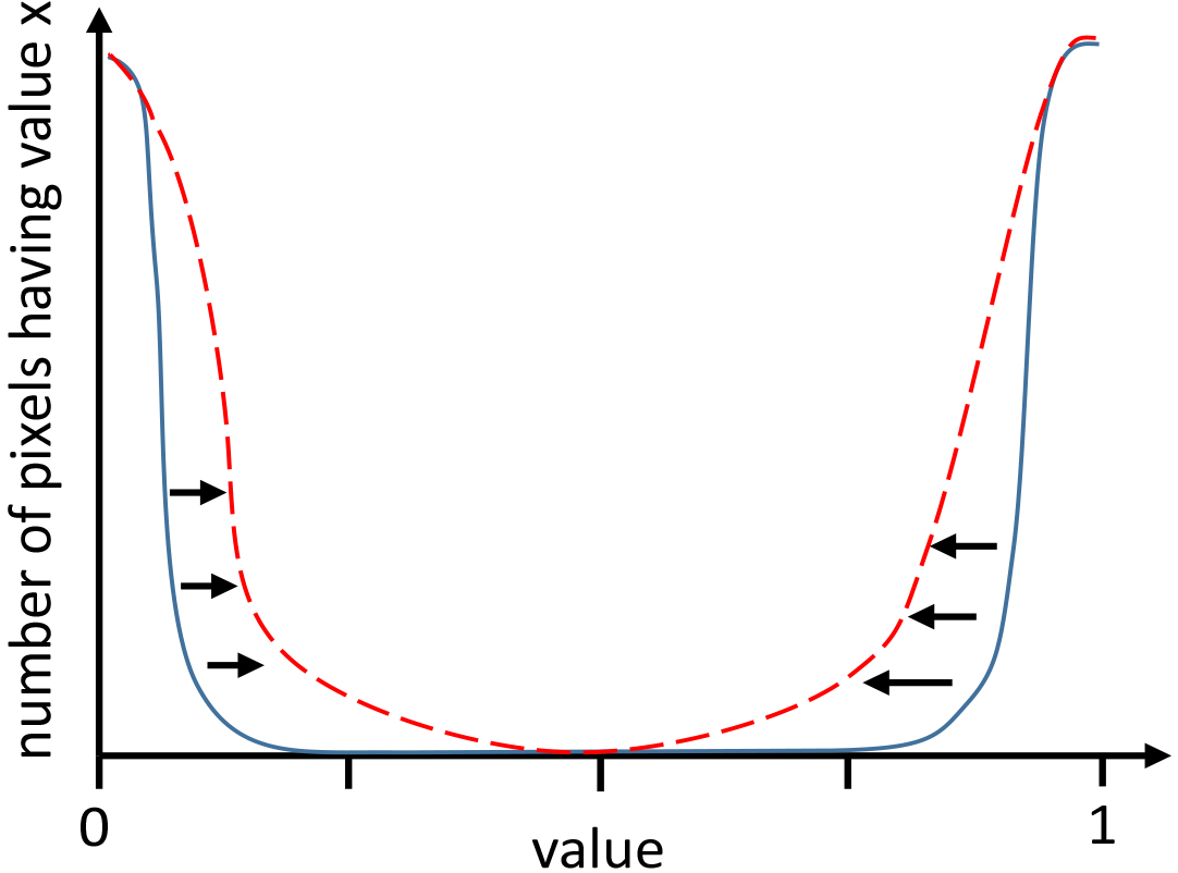

2.4 Further adaptions

Beside the entropy and the $l_{1}$ regularization, we also implemented the Total Variation Distance (TVD) for testing. It was developed for denoising in images like in [35]. TVD follows the assumption that noise in images can be described as high differences between adjacent pixels. Hence, it is able to reduce the gradient between adjacent pixels. Including it into the cost function with a quantifier $\lambda_{V}$ may help to extract less noisy filters and better patterns. It is defined as:

$\displaystyle\textit{TVD}=$ $\displaystyle\sum_{n=1}^{nf}\sum_{i=1}^{h-1}\sum_{j=1}^{fl-1}\sqrt{\left|w(n,i% +1,j)-w(n,i,j)\right|^{2}}$ $\displaystyle\overline{+\left|w(n,i,j+1)-w(n,i,j)\right|^{2}}$ (7)

In theory this could help especially in time series images with a high number of bins. If there are too few bins, the smoothing by TVD may add too much dissimilarity. The use of entropy and TVD at once may also cause problems, because they are optimizing against each other. As shown in Fig. 4 the entropy pushes the frequency distribution of the pixel values to 1 and to 0. On the contrary the TVD smoothes the pixel-gradients and therefore also changes the distribution to the middle. The overall cost function with all regularizations now results to:

$\displaystyle\textit{cost}=\textit{MSE}+\frac{\lambda_{L,dyn}}{\textit{NW}}% \cdot l_{1}+\lambda_{E}\cdot\textit{ENT}+\lambda_{V}\cdot\textit{TVD}$ (8)

Furthermore we added a dropout layer to the CAE architecture between the sparsity and the deconvolutional layer. The dropout technique randomly sets a certain percentage (dropout rate) of weights to zero within every iteration of learning, which helps to find the global minimum of the cost function.

On top of these adaptions we enabled GPU computing for CAE by the use of TensorFlow-GPU. For the following evaluations in Section 4.2 we use a nVidia Quadro P6000.

3. Recently proposed approaches for pattern discovery

The following nonlearning approaches for pattern discovery in time series were already proposed in previous work [3] and are now considered as relevant references for the NN-based approach proposed in Section 2. For better understanding Section 3.1 to 3.3 again describe those three nonlearning approaches.

3.1 DTW-based

The tested implementation is based on the approaches from [21, 22]. We are using the scoring function of the CrossMatch algorithm, which is necessary to compute the matrix equivalent to the DTW algorithm. In the case of CrossMatch the matrix contains values of similarity in contrast to the DTW which computes a distance matrix. The scoring function for every cell $(i,j)$ of the similarity matrix $v$ of CrossMatch using the time series $x$ and $y$ is shown in the following equation:

$\displaystyle v(i,j)=$ $\displaystyle\quad\textit{max}\left\{\begin{array}[]{l}\varepsilon b_{d}-\left% \|x_{i}-y_{i}\right\|+v(i-1,j-1)\\ \varepsilon b_{v}-\left\|x_{i}-y_{i}\right\|+v(i,j-1)\\ \varepsilon b_{h}-\left\|x_{i}-y_{i}\right\|+v(i-1,j)\\ 0\end{array}\right.$ (9)

In general, CrossMatch is made to find similar subsequences within long time series $x$ based on a reference time series $y$ . In Fig. 5 an example of a similarity matrix is given that was calculated by CrossMatch. It calculates a similarity for every possible sample combination of $x$ and $y$ , beginning in the lower left corner. Every calculated similarity $v(i,j)$ of $x_{i}$ and $y_{j}$ is dependent on the preceding values in the similarity matrix. Following this approach similar subsequences can be identified, as shown in Fig. 5 by green and red circles, marking the beginning and ending of each similar subsequence.

Figure 5.

Visualization of the similarity matrix $v$ of a short reference time series $y$ and a longer time series $x$ calculated by CrossMatch scoring function. The green circles mark the beginning of a similar subsequence within the longer time series regarding the reference time series. Accordingly, the red circles mark the end of similar subsequences.

A major difference between the scoring functions of the classic DTW and CrossMatch is the usage of weighting factors $\varepsilon b_{d}$ , $\varepsilon b_{v}$ and $\varepsilon b_{h}$ . It enables us to penalize time scaling, i.e. horizontal or vertical steps in the similarity matrix. While DTW is only able to calculate a distance between two sequences, CrossMatch enables the detection of motifs as well. The end of a motif is marked by a local maximum in the similarity matrix $v$ . Furthermore the CrossMatch algorithm calculates a position matrix, which contains the starting points of the motifs. For further explanations of DTW and CrossMatch, see [36] resp. [21].

For the tests, that we are going to perform, we limit the weighting factors to $\varepsilon b_{d}=1$ , as a reward for similarity, and $-1\leqslant\varepsilon b_{v}=\varepsilon b_{h}\leqslant 0$ , as a possible penalization for time scaling. Furthermore we need to make an adaption to the CrossMatch scoring function, see Eq. (10). In order to search for motifs in one and the same time series, we have to exclude the trivial matches. Therefore we implement an offset region around the diagonal of the similarity matrix $v_{\textit{adapt}}(i,j)$ . These matrix cells are set to zero by default. Due to symmetry only half of the matrix has to be calculated. These adaptions also apply to the position matrix.

$\displaystyle v_{adapt}(i,j)=\left\{\begin{array}[]{ll}v(i,j)&\text{if}\left|i% -j\right|>\textit{offset}\\ 0&\text{if}\left|i-j\right|\leqslant\textit{offset}\end{array}\right.$ (10)

In order to form patterns, additional to the CrossMatch, we extract and cluster the motifs like in [22]. To extract possible pattern candidates from the matrix, we use a minimum length and a minimum similarity. This process is exemplarily shown in Fig. 6. Both axis of the similarity matrix refer to one and the same time series $x$ . The green and red markers highlight the extraction of one pattern candidate. Every candidate’s score higher than the product of min_length and min_similarity is going to be clustered. The clustering algorithm needs another parameter specifying the sensitivity of the extracted motifs to be clustered to patterns, which is later referenced to max_similarity_motif. To ensure that every subsequence in the time series similar to the pattern is discovered, a representative sequence of each pattern is extracted and searched in the whole time series by recalculating the CrossMatch similarity matrix.

Figure 6.

Visualization of the similarity matrix 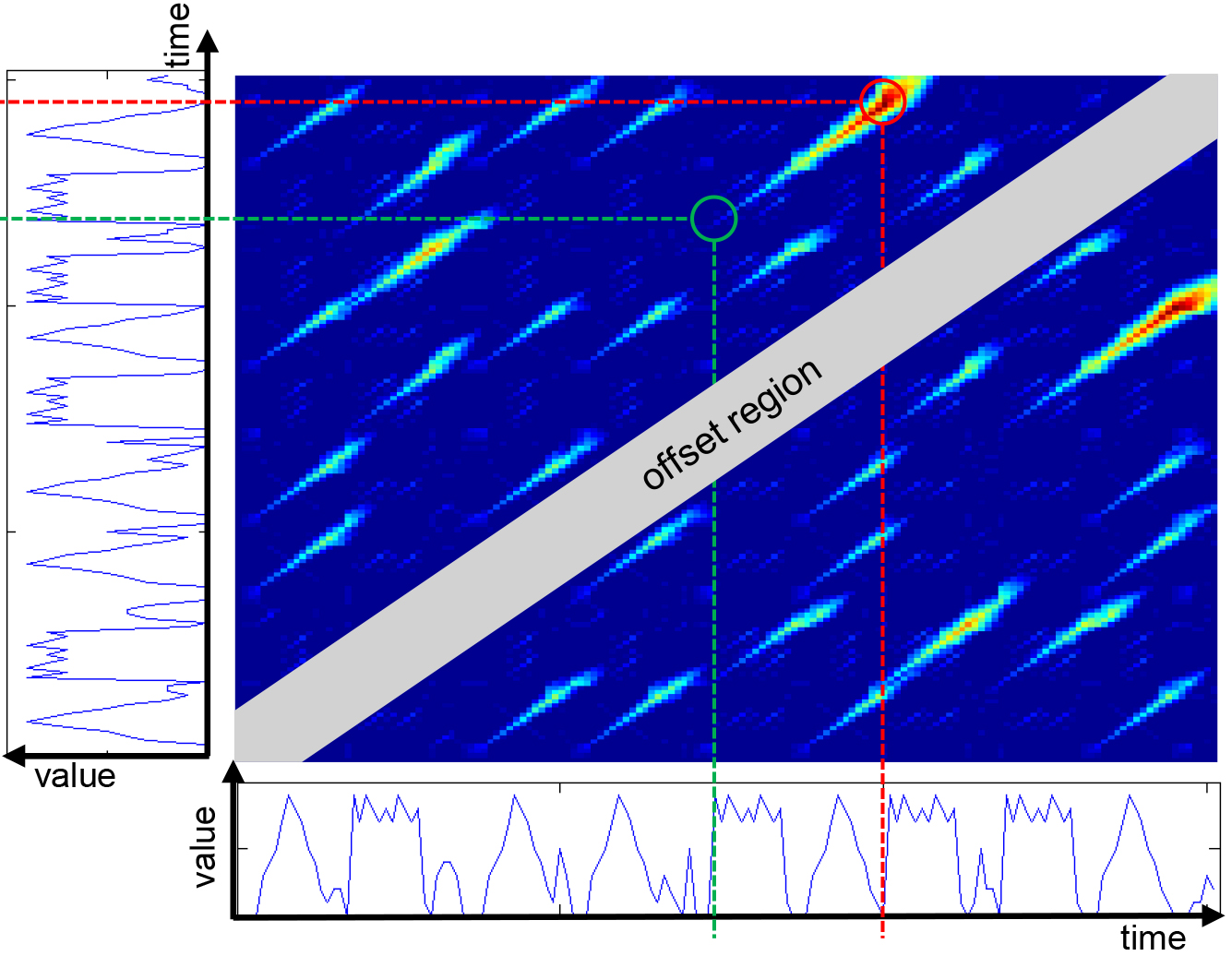$v$ to find patterns in $x$ .

3.2 Discretization-based

Concerning discretization-based approaches for pattern discovery we focus on an adapted Sequitur algorithm and an algorithm for pattern enumeration. Both are based on an equal probability discretization technique. However, in contrast to the technique described in [23], we do not assume a Gaussian distribution of the data values, which is necessary in terms of various signal types. We implemented a simple algorithm to form classes of equal count of data points with respect to the constraints uniqueness and allocation. Uniqueness means that there must not be multiple classes with the same data value. According to the allocation constraint, every data value has to be allocated to one class. The algorithms, which will be described shortly, are only dependent on one parameter, the number of discretization steps.

Figure 7.

Exemplary visualization of three similar subsequences, their unreduced symbolic representations as well as the symbolically reduced representation.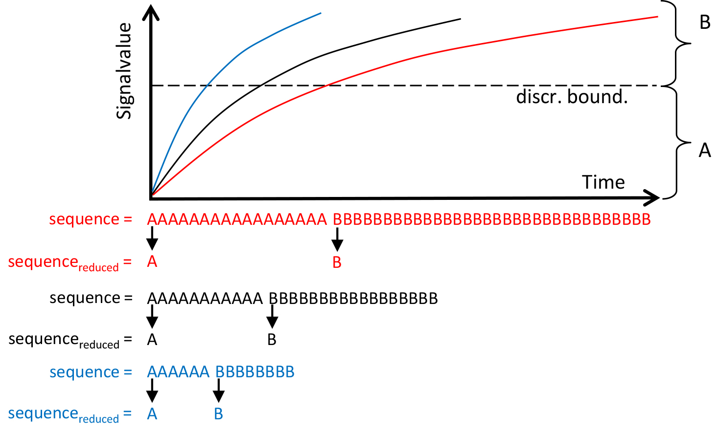

Because of the need of time scaling we apply an optional numerosity reduction technique like in [2], which we call symbolic reduction. Therefore every identical consecutive symbol in the time series is reduced to one unique symbol. Hence, in every step of the time series a change in the symbolic value can be observed. In Fig. 7 the discretization and symbolic reduction of three similar subsequences is shown. For simplicity the signal is discretized into two symbols $A$ and $B$ . As already mentioned every sample is assigned to one of the symbols. The sequences of identical consecutive symbols are reduced to one of its kind to get the reduced symbolic time series. Without reduction these three sequences could not be identified as patterns, because the following algorithms, pattern enumeration or Sequitur, are only able to identify identical sequences as patterns. Hence, by the use of symbolic reduction similar sequences that are scaled in time can be identified as patterns. A beneficial side effect is the compression of the time series, which leads to faster execution of pattern discovery. On the downside, the pattern discovery algorithm now completely ignores every temporal information, which can cause extreme duration variation within the members of a pattern.

3.2.1 Pattern enumeration algorithm

To evaluate the performance of our adapted Sequitur algorithm, we also want to apply a pattern enumeration algorithm. The algorithm repeatedly scans the whole time series with different query pattern lengths by using a matrix representation of the symbolic time series and a sorting algorithm. While scanning through all lengths, every pattern that occurs at least 2 times is stored in a dictionary. In text mining this kind of approach is often named as word count. In Algorithm 1 the approach of pattern enumeration is shown.

Pattern Enumeration[1] PatternEnumeration $s t s$ $l\textit{\_pattern}=1$ $\textit{empt}=\textit{false}$ $\neg\textit{empt}$ $l\_\textit{pattern}=l\_\textit{pattern}+1$ $ts\_\textit{matrix}=\textit{form\_matrix(sts, l\_pattern)}$ $[ts\_\textit{matrix\_sorted, index}]=\textit{sort(ts\_matrix)}$ $[\textit{sym\_repr, num, loc}]=$

get_symbolic_repr(ts_matrix_sorted) $p\leftarrow 1,\textit{length(sym\_repr)}$ $\textit{num}(p)>1$ $\textit{add2dict(sym\_repr}(p),\textit{loc}(p))$ $\textit{isempty}(\textit{find}(\textit{num}>1)$ $\textit{empt}=\textit{true}$

Lines 6 to 8 are the core of the algorithm. In line 6 the time series array is transformed to a matrix of the size $(\textit{length(sts)}-\textit{l\_pattern}+1)*\textit{l\_pattern}$ . The variable l_pattern describes the length of the patterns that are searched in the current iteration of the WHILE loop. In the function form_matrix the symbolic time series sts gets multiplied l_pattern times and shifted by a number of entries dependent on the column. This leads to matrix rows with consecutive symbolic values. In line 7 the matrix is sorted along the first dimension, which leads to a matrix with equal row values located in consecutive rows. By detecting changes along the sorted matrix within the function get_symbolic_repr, all the patterns and their symbolic representations can be extracted. Furthermore the number (num) and the location (loc) of the occurrences can be identified. In the last step every detected pattern with a count greater than one is documented in a dictionary. The dictionary contains every detected pattern and its location. The algorithm terminates if in the current iteration of the WHILE loop no pattern is found.

3.2.2 Adapted Sequitur algorithm

The Sequitur algorithm proposed in [25] is based on two constraints. The first constraint is called digram uniqueness, which means that every digram (a pair of two adjacent symbols) is allowed to occur only once in the symbolic time series. If a digram appears more than once, then a rule is created that replaces the digram by a new symbol. All the rules are stored in a dictionary. Every rule has to fulfill the second constraint, the rule utility. It says that every rule has to occur at least twice. In Fig. 8 an exemplary execution of the algorithm is shown based on a symbolic sequence, that grows in every iteration by a new incoming symbol. In every iteration the extracted grammar, the dictionary, is updated under consideration of both constraints.

Figure 8.

Execution of the original Sequitur algorithm on a sequence of symbols [25].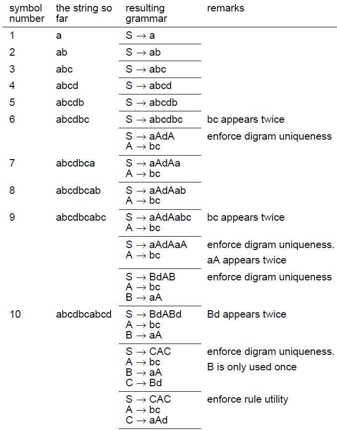

Our adaption of the algorithm is shown in Algorithm 2. Since the original Sequitur algorithm is a streaming algorithm, which is not the focus of this work, the adapted Sequitur implements the approach in an offline fashion. The first three steps within the WHILE loop are similar to the pattern enumeration algorithm, except for a fixed matrix column size of 2. To fulfill both, the diagram uniqueness and the rule utility, the algorithm adds the digram that occurs the most to the dictionary and replaces the diagram in the symbolic time series by a new symbol. While the original Sequitur replaces the rule that occurs first, due to the streaming approach, the adapted Sequitur opens up the opportunity to choose the next rule. In this implementation the digram that occurs the most is chosen to be replaced in line 8. The algorithm terminated when the diagram uniqueness is fulfilled.

Adapted Sequitur[1] AdaptedSequitur $s t s$ $\textit{empt}=\textit{false}$ $\neg\textit{empt}$ $\textit{ts\_matrix}=\textit{form\_matrix}(\textit{sts},2)$ $[\textit{ts\_matrix\_sorted, index}]=\textit{sort(ts\_matrix)}$ $[\textit{sym\_repr, num, loc}]=$

get_symbolic_repr(ts_matrix_sorted) $\textit{max(num)}>1$ $[v,i]=\textit{max(num)}$ add2dictionary(sym_repr(i), loc(i)) $\textit{sts}=\textit{replace\_by\_newrule(sts, loc)}$ $\textit{empt}=\textit{true}$

3.3 Matrix profile

Matrix Profile introduced in [29] is an approach able to be executed on raw time series without any preprocessing. Matrix Profile is based on the calculations of distance profiles, which is exemplarily shown in Fig. 9. A distance profile $D$ visualizes the distances between a query sequence $Q$ and every other possible sequence in a time series $T$ (with $\textit{length(timeseries)}\gg\textit{length(query)})$ while the query sequence is part of the time series and all the compared sequences have the same length. Thus the minimum of the distance profile, excluding the trivial match, is the best match with the query sequence. To extend the distance profile to a Matrix Profile MP, a distance profile for every possible query is calculated. The minimum of every distance profile is visualized in the Matrix Profile. Additionally a vector is needed to store the index information of its nearest neighbor sequence. For further details see [29].

Figure 9.

Distance profile $D$ (bottom) of an exemplary time series $T$ (top) and a query subsequence $Q$ [29].

To extract motifs of a fixed length a maximum distance threshold is needed for two sequences being a motif. Because all the minimum distances are stored in the Matrix Profile, every entry and its corresponding subsequences that fulfill this constraint can be seen as motifs. The corresponding distance profile gives information about other sequences that are similar to the motif. Again every data point that falls below the maximum distance leads to a similar sequence. The motif with its similar sequences can then be called a pattern. To discover patterns without a fixed query length we have to apply the algorithm multiple times for a set of possible query lengths. [29]

Because of the naïve structure of the approach, the MASS algorithm was proposed in [29], which calculates the z-normalized Euclidian distance profile by convolution. In comparison to the naïve approach of calculating the Euclidian distance between the query and every other sequence, this technique reduces the time complexity for a distance profile from $O(n*m)$ to $O(n*log(n))$ with $m$ being the length of the query and $n$ the length of the whole time series. However, for time scaled pattern discovery the Euclidian distance is not suitable. An alternative solution is to replace it by DTW, which theoretically increases the complexity to $O(n*m^{2})$ . For the calculation of a Matrix Profile we have to calculate approximately $n$ distance profiles, which leads to a complexity of $O(n^{2}*m^{2})$ . As we want to find patterns without input of a query length the Matrix Profile has to be calculated multiple times for different query lengths [29].

In a second implementation we tested Matrix Profile with the Euclidean distance but reduced complexity. It is based on the fact that the distance profiles of the query at starting point $i$ and the one at starting point $i+1$ have $\textit{query\_length}-1$ identical parts in the Euclidean distance calculation. While calculating the distance profiles in serial, it is possible to keep these identical parts and calculate the next distance profile with just two additional computation steps per data point in the distance profile.

4. How to compare different approaches/ algorithms?

In this section we discuss a testing standard for the comparison of different approaches. One possibility is to use benchmark time series, for example from financial stock markets or from seismology, which are commonly used to test different time series exploration tools. However, generalized results regarding every possible kind of pattern can be obtained only by use of synthetically created time series. Our test data is composed of predefined patterns, which can be labeled automatically, as described later on in Section 4.1. The advantage of this approach is the independency of a certain test case. Furthermore we can create an infinite number of test sequences without the effort of labeling it.

The evaluation is divided in three steps. In the first step the test data is created automatically from patterns that are generated randomly. In the second step, the pattern discovery, the predefined patterns are rediscovered using different algorithms and parameter settings. By using the index information of every predefined and located pattern, in the third step quality scores for the results are calculated.

4.1 Time series test data creation

For a generalized evaluation for various use cases, the test patterns should cover every possible kind of shape. That is why we chose the random walk as the basis for every pattern. In our case we use a Gaussian random walk, which changes the distribution of the randomly chosen step size from equal to normal. For the creation of a primal pattern by a Gaussian random walk the following parameters are also chosen randomly once: Value of the first data point; number of steps; maximum step size.

After creating different primal patterns, each of them is multiplied and distorted to form a set of similar members for each of the primal pattern. The number of members within a pattern is randomly chosen. The distortion is done by adding white Gaussian noise to the members, given a fixed signal to noise ratio, and by randomly stretching or compressing the length of the members, given a maximum ratio between the length of the primal pattern and the distorted member.

To form a sequential time series based on the randomly created patterns and its members, the members are concatenated in a random order. Note that every member can only occur once in the time series. To overcome value jumps between the concatenated patterns, we insert a smooth crossing. Start and end indices of every member and every pattern are saved.

4.2 Pattern evaluation

Output of the pattern algorithms are indices of starting and ending points of the located pattern. To evaluate the rediscovered patterns we calculate different quality scores comparing these indices $I_{\textit{loc}}$ with the indices of the predefined pattern $I_{\textit{pre}}$ . The overlap, the True-Positive-Rate (TPR) and the False-Discovery-Rate (FDR) are defined as:

$\displaystyle\textit{overlap}=\frac{\left|\textit{TP}\right|}{\left|\textit{TP% }\cup\textit{FN}\cup\textit{FP}\right|}=\frac{\left|\textit{TP}\right|}{\left|% I_{\textit{pre}}\cup I_{\textit{loc}}\right|}$ (11) $\displaystyle\textit{TPR}=\frac{\left|\textit{TP}\right|}{\left|\textit{TP}% \cup\textit{FN}\right|}=\frac{\left|\textit{TP}\right|}{\left|I_{\textit{pre}}% \right|}$ (12) $\displaystyle\textit{FDR}=\frac{\left|\textit{FP}\right|}{\left|\textit{TP}% \cup\textit{FP}\right|}=\frac{\left|\textit{FP}\right|}{\left|I_{\textit{loc}}% \right|}$ (13)

with: $\textit{TP}=I_{\textit{pre}}\cap I_{\textit{loc}}$ ; $\textit{FP}=I_{\textit{loc}}\setminus I_{\textit{pre}}$ ; $\textit{FN}=I_{\textit{pre}}\setminus I_{\textit{loc}}$ .

In Fig. 10 these index sets are exemplarily visualized for one member of a predefined and a discovered pattern. The dashed line shows the time series, while the blue line is the predefined pattern and the red line is the discovered pattern. In fact, the members of a pattern are not handled separately as shown in Fig. 10, but all simultaneously. Hence, $I_{\textit{loc}}$ for example contains all the indices of all members of one discovered pattern. An overlap score of 0 describes a mismatch and a score of 1 describes a perfect match between predefined and discovered pattern. Note that the overlap also decreases from a perfect match if the detected pattern is longer than the predefined one. The calculation is performed for every combination of predefined and detected pattern. Afterwords a best match for every predefined pattern can be chosen. To express an one-score quality criterion for the algorithms, we chose the mean overlap value of the best matches. Although in the evaluation, following in Section 5, we will focus on the overlap for the main quality score, the FDR and TPR also contain valuable additional information.

Figure 10.

Exemplary visualization of index sets for the calculation of overlap, TPR and FDR.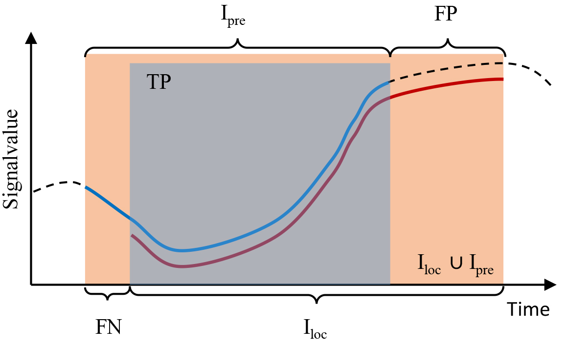

Figure 11.

Overview of different approaches concerning overlap and runtime; length of datasets ca. 50.000 data points; average count of located patterns: DTW ca. 800; Pattern Enumeration 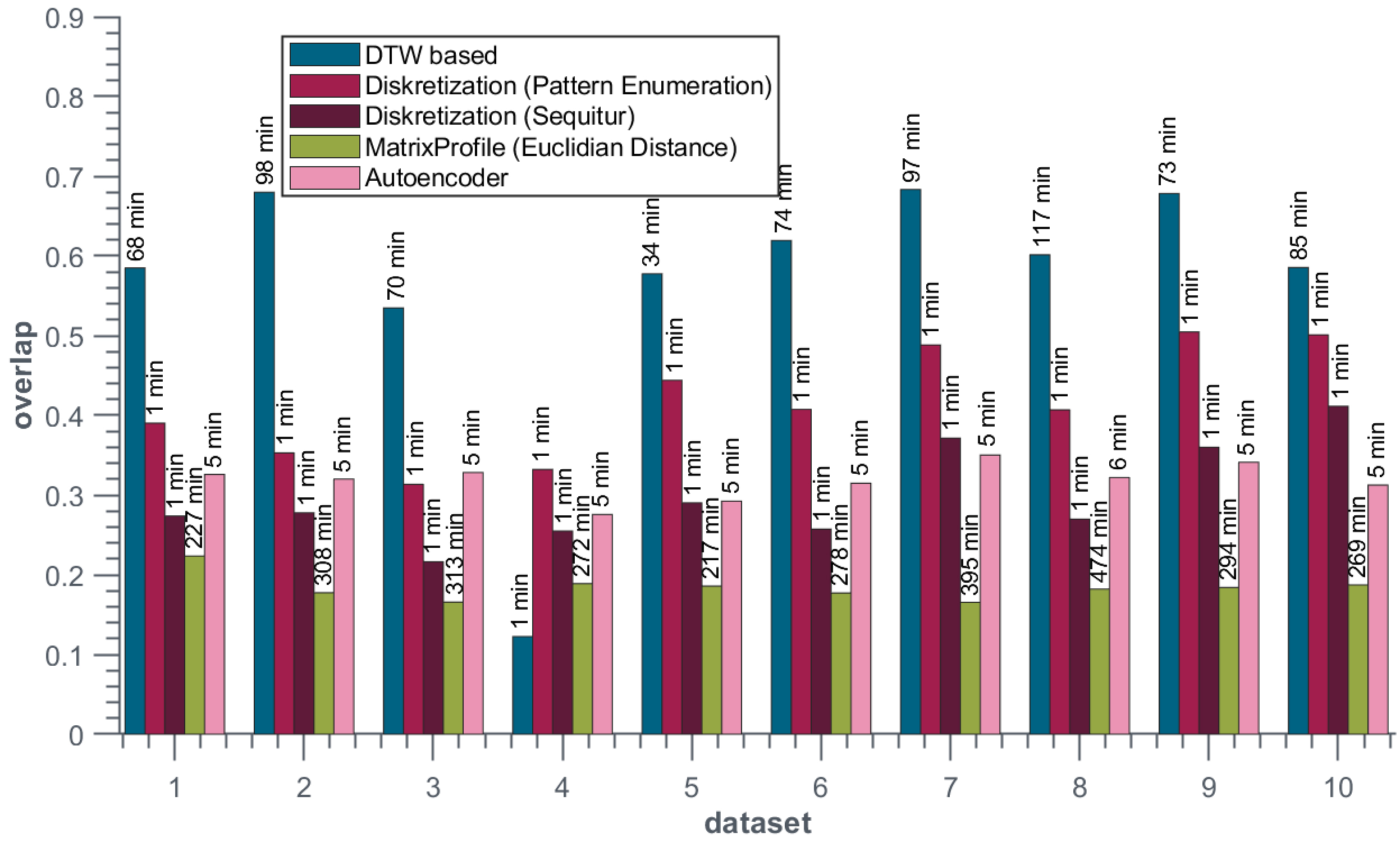$>$ 20.000; adapted Sequitur ca. 200; Matrix Profile $>$ 50.000; Autoencoder ca. 700.

Furthermore we perform the whole routine 10 times, to get a reliable statement for the quality of the algorithms. This gives us also the possibility to make a statement concerning the variance of the quality. Beside this, in every iteration of the routine, the computing time of the different algorithms is recorded.

5. Experimental evaluation

After explaining the different approaches for the pattern discovery and the methodology of calculating the quality scores, we now compare the different approaches. In Section 5.1 at first all the approaches are ranked based on synthetic data sets. In Section 5.2 follows a more detailed evaluation of the CAE. Sections 5.3 to 5.5 briefly deal with a separate evaluation of nonlearning approaches. Finally in Section 5.6 the approaches are exemplarily applied to a real life vehicle data set.

5.1 Comparison of best results

We created 10 random datasets each containing approximately 50k samples, ran every algorithm with different parameter settings and calculated the quality scores. For each algorithm we chose the parametrization leading to the best results, see Figures 11 and 12. In the upper plot of Fig. 12 these best results are visualized concerning the overlap and the runtime with different markers showing the corresponding approaches. Furthermore, the circled markers show the mean value of the approaches for all datasets. The standard deviation is highlightes as circle arround the mean value. Likewise, the lower plot shows the FDR and TPR.

Figure 12.

Top: Vizualization of overlap and runtime for best parametersets including a marker for the mean value and a circle arround it showing the standard deviation for each approach; Bottom: Equivalent vizualization of TPR and FDR.

It is evident that the DTW-based approach outperforms every other tested approach concerning overlap and TPR. Discretization-based approaches, in turn, advance greatly concerning the runtime. The algorithm for pattern enumeration provides constantly better results than the Sequitur algorithm, except for the runtime. CAE produces a similar quality like the discretization-based approaches concerning overlap, TPR and FDR. But while CAE needs around 5 minutes for the datasets to process, the discretization-based approaches take only seconds. Here we need to point out, that the number of patterns identified by the pattern enumeration algorithm is extremely high. On the one hand this leads to a better quality in comparison to the Sequitur algorithm. But on the other hand this makes it hard to handle and implies the need for post processing methods.

As expected, the Matrix Profile with the use of the Euclidean distance is not able to compete with the other approaches because of its complexity and the inability of time scaling. We expect better results when using the Matrix Profile in combination with DTW instead of the Euclidean distance, though substantially increasing runtime. As the Matrix Profile is outperformed by every other approach, it is not suitable for our use cases. However, as we calculated an entire Matrix Profile for every possible query length, there is still optimization potential for reducing the runtime based on early abandoning. Nonetheless this reduces the runtime, but does not improve the overlap.

It is highly desirable to have a method that produces results with constant quality. As highlighted in Fig. 12 the DTW-based approach shows the highest standard deviation and, hence, the greatest variation in quality. This is mainly caused the bad performance regarding the dataset 4 (see Fig. 11). Excluding this run from the analysis would then result in a standard deviation similar to the value of discretization-based approaches. Furthermore, it is worth noting that CAE shows relatively low standard deviation in every dimension, even though its learning technique is nondeterministic.

5.2 Evaluation of CAE

The biggest challenge in applying CAE for pattern discovery is the choice a of good working parameter setting. In theory 14 parameters have to be chosen to parametrize CAE. After pretuning CAE we focused on varying 6 out of 14 parameters, which are listed in Table 1.

Table 1
Overview of varied parameters for the experiments of CAE

Parameter	Varied
Batch size	X
Number of epochs	X
Length of input time series image (document size)	X
Height of filters, number of bins $h$	$\surd$
Variation of filter length (minimal length, maximal length, $\Delta fl$ )	X
Number of filters $n f$	X
Dropout rate	$\surd$
Quantifier of dynamic L1 regularization $\lambda_{L,dyn}$	$\surd$
Quantifier of TVD regularization $\lambda_{V}$	$\surd$
Quantifier of entropy regularization $\lambda_{E}$	$\surd$
Latent limit	X
Learning rate	$\surd$

Figure 13.

Results of CAE in overlap, runtime, TPR and FDR varying all 6 parameters. The difference in selecting the Entropy or the TVD is highlighted including a variation of the number of bins; Top: Vizualization of overlap and runtime; Bottom: Vizualization of TPR and FDR.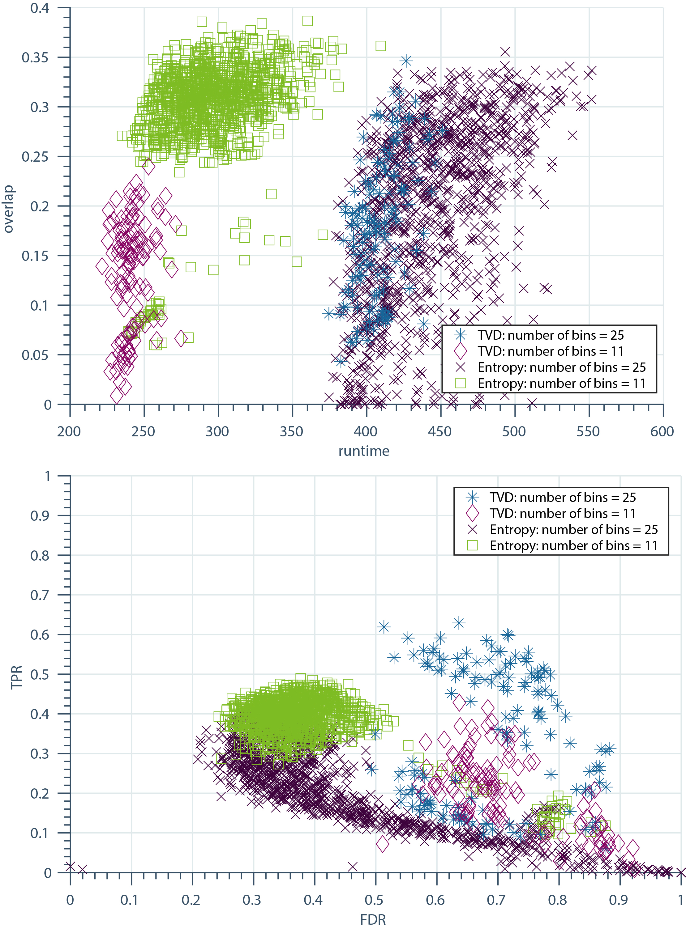

In general we experienced the dropout layer to be very effective in avoiding local minima and leading to good results of the pattern discovery. In most cases a dropout rate between 0.2 and 0.25 had the best impact. Furthermore, applying the $L1$ regularization is one of the keys in this NN-based approach. Our proposed dynamic adaption of $L1$ works as desired and is crucial when using CAE for variable length pattern discovery.

Figure 14.

Visualization of 10 independend runs of the best parameterset (Autoencoder) for datasets 1-5 including a marker for the mean value and a circle arround it showing the standard deviation for each dataset; Top: Vizualization of overlap and runtime; Bottom: Vizualization of TPR and FDR.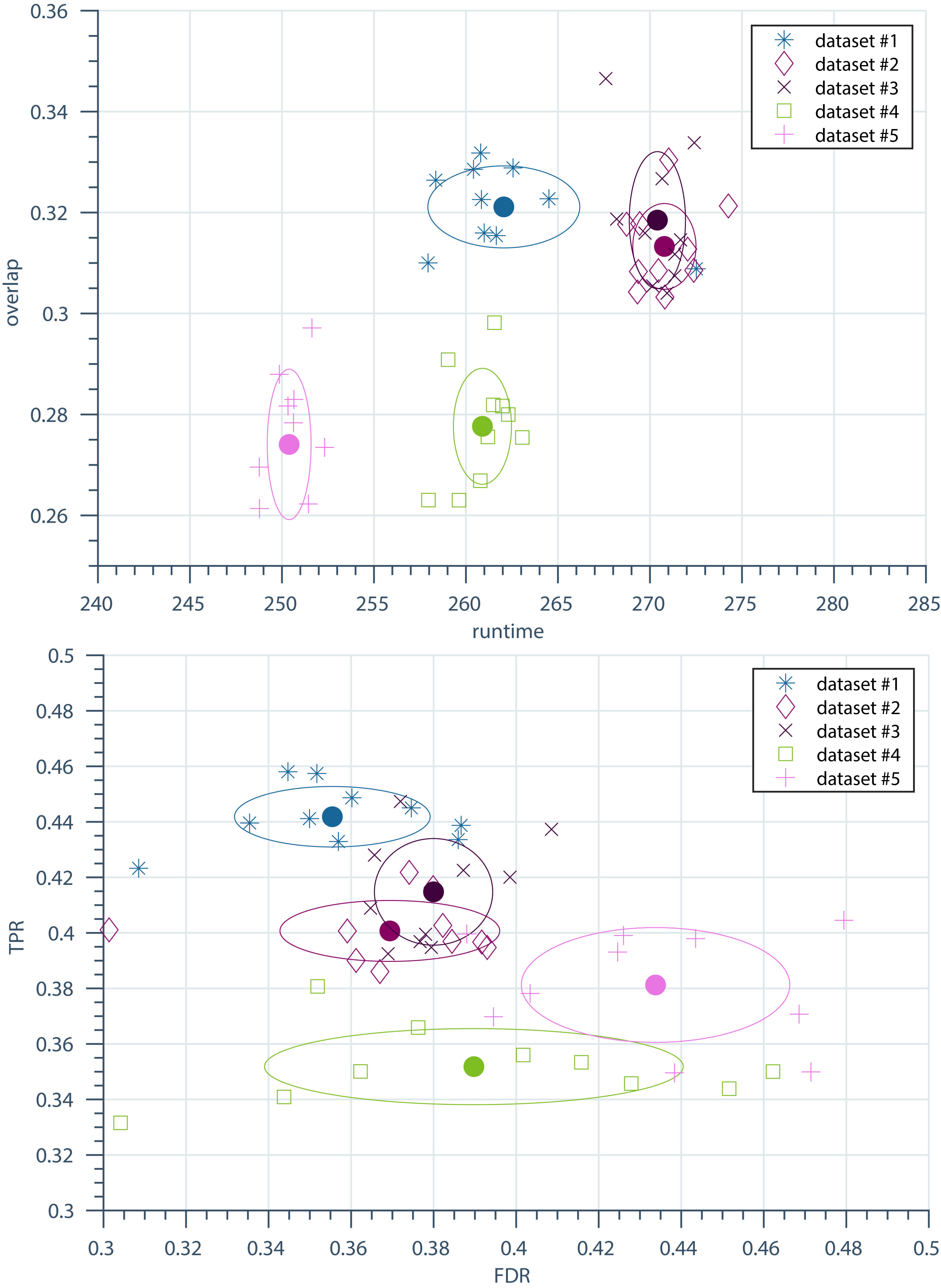

A major question was the functionality analysis of the entropy and the TVD regularization. Both methods can separately add value to the quality of patterns. As already described in Section 2.4 the use of entropy and TVD at once causes problems, due to their opposed objectives. We tested both alternatives with many different parameter settings to evaluate their effect in overlap, runtime, TPR and FDR. The result is shown in Fig. 13. Additionally the variation of number of bins is highlighted. Our previous assumption in Section 2.4 turned out to be correct: TVD works better when using a higher number of bins. CAE with the use of TVD is able to produce a higher overlap and TPR with 25 bins than with 11 bins. When analyzing the entropy the results are switched. Hence, the results are better when using a lower number of bins. In general CAE runs faster the lower the number of bins is. Comparing both approaches, it is shown that the TVD has a higher FDR in both cases (11 and 25 bins) than the entropy. Furthermore the results of entropy are in the best cases noticeably better in terms of overlap while also requiring less computing time. Regarding the overlap, even if both approaches run with 25 bins, the entropy is able to produce an equal or slightly better result.

Figure 15.

Results of DTW-based algorithm (10 random datasets), for every costwarp parameter value a separate plot; top: mean overlap of random datasets with different parameters; bottom: mean runtime in minutes.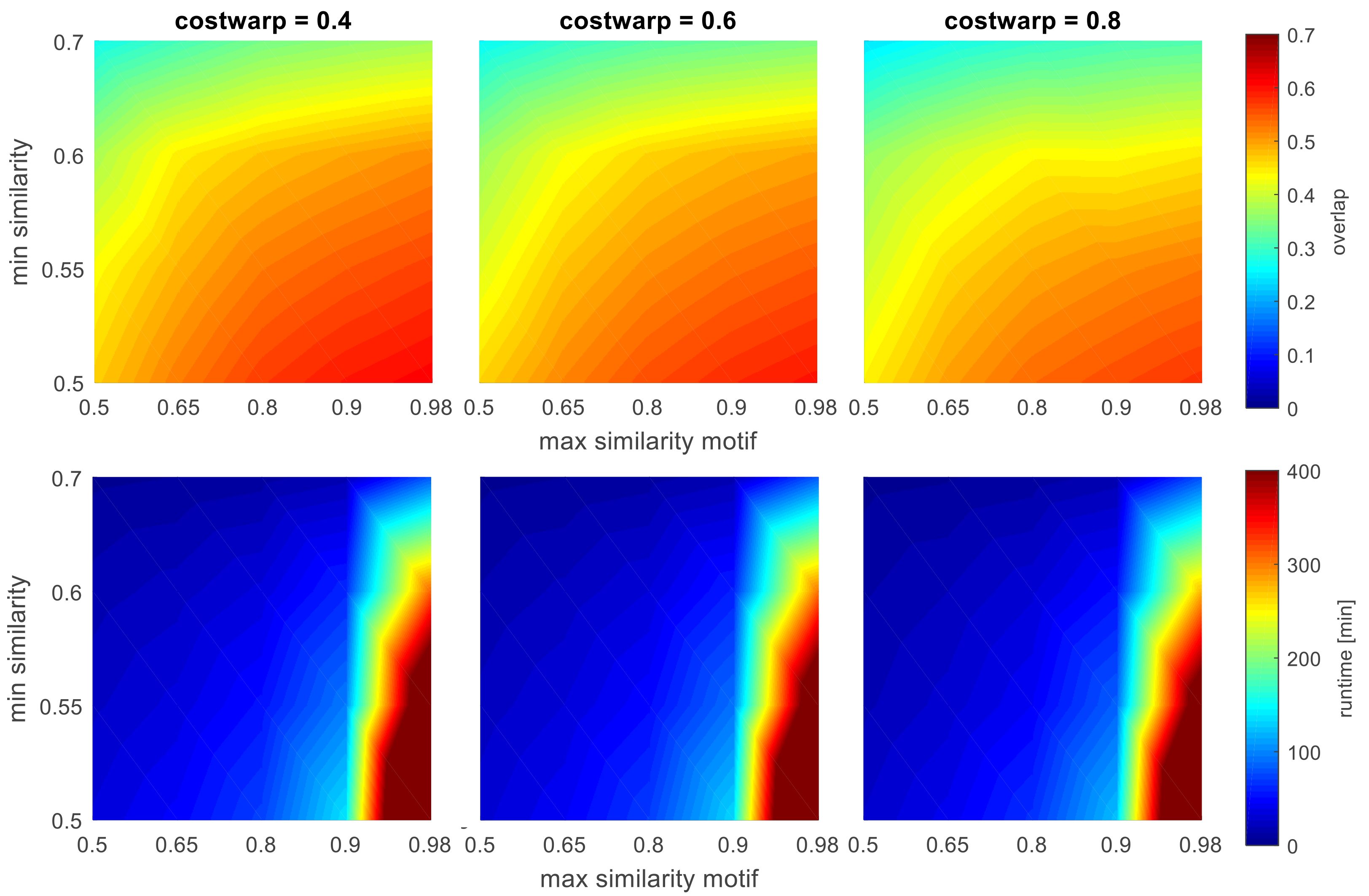

In contrast to nonlearning approaches for pattern discovery, CAE has the problem of nondeterminism, because of the randomly initialized weights of the convolutional and deconvolutional filters. We ran the best parameter setting for every dataset 10 times to estimate the influence of the randomly initialized weights. In Fig. 14 the results are shown for the first 5 datasets with different markers. Furthermore the mean value is visualized by the corresponding encircled marker. The maximum deviation for the overlap is 0.04, which could cause problems in use cases that require reproducibility. The ability to transfer a good working parameter setting to another dataset is given, if the datasets are from the same kind, e.g. time series of similar lengths containing information about the same sensor. Hence, in the case of a synthetic time series created by the method explained above, a good parameter setting tends to produce good results in every dataset.

5.3 Evaluation of DTW-based approach

Figure 11 shows the best case results of the approaches concerning the overlap. For the DTW-based approach, for acceptable runtime we chose a compromise between acceptable runtime and high overlap. This tradeoff is shown in Fig. 15. With growing values of max_similarity_motif, the runtime increases dramatically. This is caused by the clustering of motifs located by CrossMatch. In case of high values of max_similarity_motif there are only few motifs clustered together to form patterns. This leads to a high count of patterns, which are then again searched in the whole time series. For further research it has to be evaluated if this last step of the DTW-based approach can be reduced or replaced by a powerful clustering of the candidates. It is also noticeable that the effort of parametrization is high in comparison to the other nonlearning approaches. At least three parameters have to be chosen carefully to get the expected results. As shown in Fig. 15 the highest overlap values result at values of $\textit{min\_similarity}=$ 0.5. We experienced an increase of the need of Random Access Memory (RAM) in cases of values lower than 0.5, which is not practical for our use cases.

5.4 Evaluation of discretization-based approaches

In Fig. 17 the performance of the discretization-based approaches are evaluated with respect to the variation of the number of discretization steps. Furthermore the benefit of the symbolic reduction is shown. It is visualized that the symbolic reduction has a higher impact on the results of the pattern enumeration algorithm than on the results of the Sequitur algorithm concerning overlap and runtime. However, in both cases the overlap as well as the runtime gets better with the use of the symbolic reduction, due to the time scaling. Nevertheless, compared to the DTW-based approach, it is a slight disadvantage because the time scaling is not controllable. I.e., after symbolic reduction, a symbol can represent two or considerably more identical consecutive symbols. A problem for both algorithms is the dependency of the discretization method, despite the dependency to only one parameter. Furthermore, we experienced a weakness in terms of multiple symbolic value toggling because of noise in value regions near the discretization boarders. This effect could be mitigated by applying a filter as a preprocessing step.

Figure 16.

Results (overlap and runtime) of Matrix Profile with variation of the maximum distance.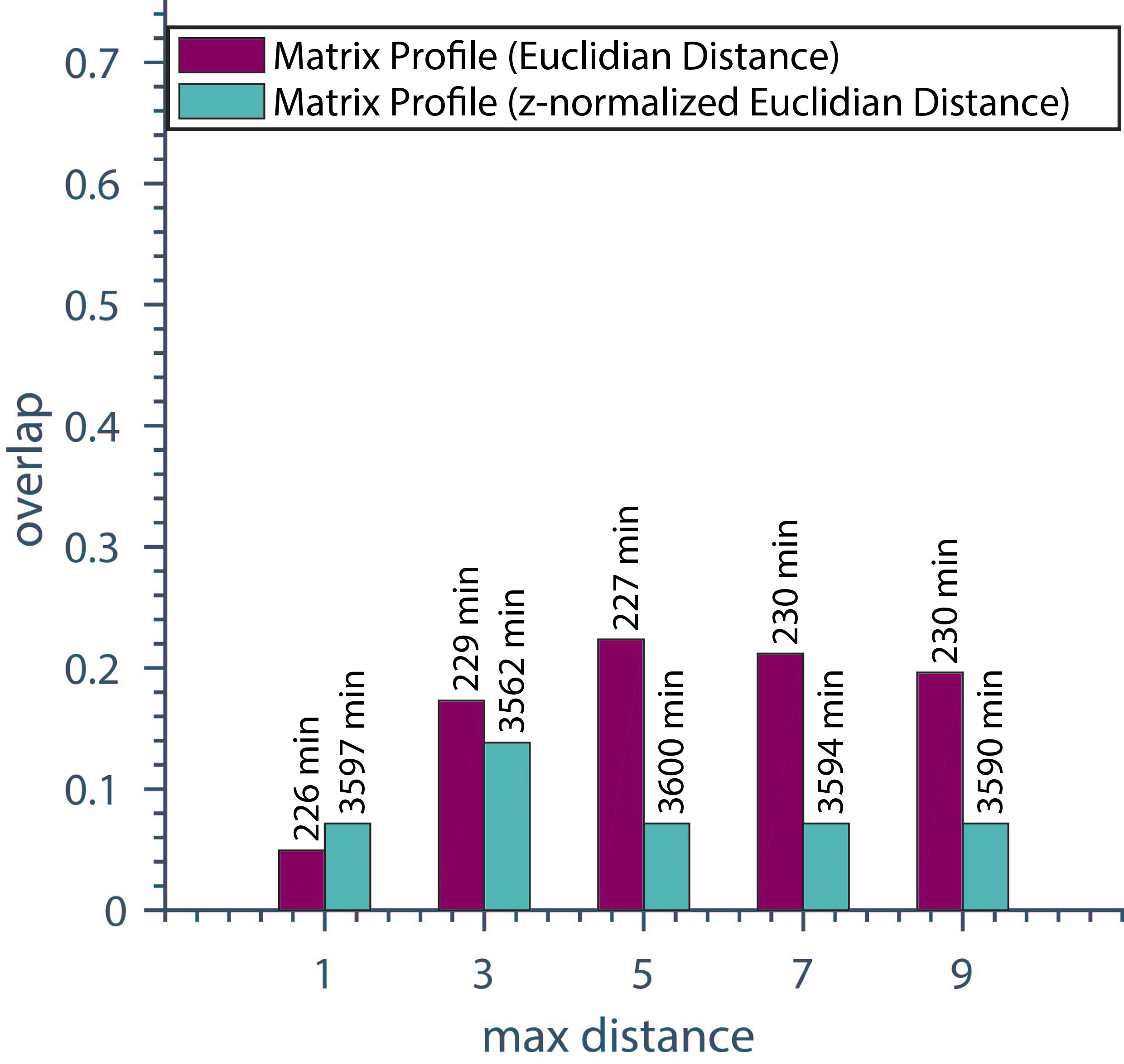

Figure 17.

Results (mean overlap and mean runtime of all datasets) of the discretization approach (Sequitur, Pattern Enumeration) with and without symbolic reduction and with variation of the discretization steps.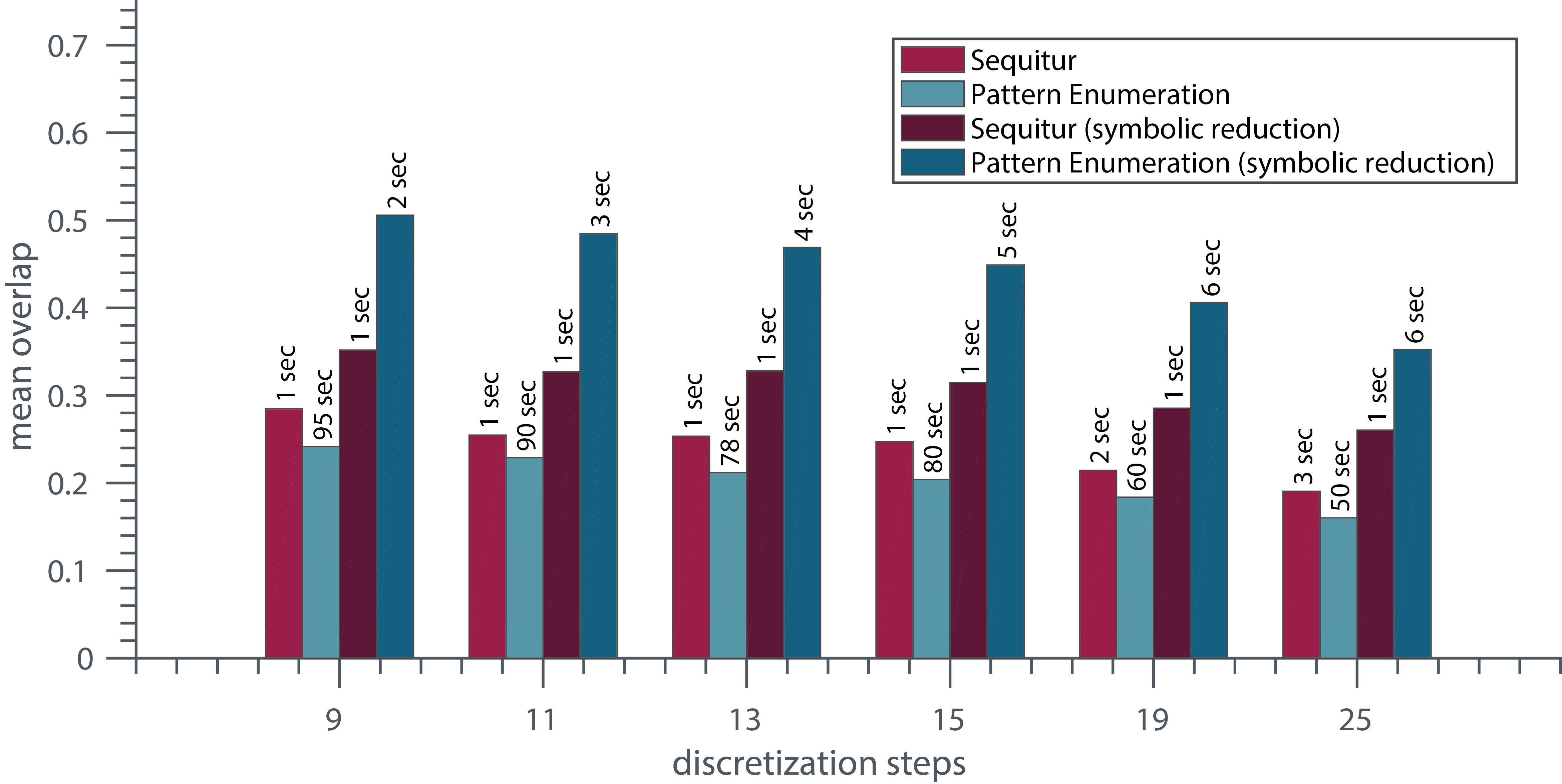

5.5 Evaluation of matrix profile

In Fig. 16 the performance of Matrix Profile with variation of the maximum allowable distance within a pattern and with use of Euclidean and z-normalized Euclidean distance is shown. The Euclidean Matrix Profile is calculated with the runtime reduction technique while the z-normalized Euclidean Matrix Profile is calculated by the MASS algorithm. As shown in Fig. 16 the Euclidean Matrix Profile leads to a better overlap for most of the parametrizations, while requiring less than 10 percent of the runtime.

5.6 Application to real Life data set

For a final validation, for each approach, we applied the best case parameter settings to a real life dataset from a typical use case in the automotive industry. It recorded the velocity of a vehicle that captured 28 hours of driving and 1 mio. samples. In general, this experiment has two major goals. First, it ought to show the applicability and transferability of all pattern discovery algorithms to data sets that are realistic in terms of size and origin. Secondly, it will show the magniture of runtime that has to be expected when applying these algorithms.

Table 2
Exemplary results for real data set

Approach	Runtime	Numb. of patterns
DTW	142 min	1,041
Matrix profile	31 hours	99,718
Pattern enum.	18 seconds	46,813
Sequitur	1 second	386
Autoencoder	48 min	144

Table 2 and Fig. 18 show exemplary results for each algorithm, which were produced with the formally determined best case parameters. While the parameters of nonlearning approaches can be easily transferred from the synthetic case to a real life data set, the parameters for CAE need to be adapted. This is a major drawback when considering CAE for the task of pattern discovery and again shows the sensititivy of its performance regarding parameter variations. With identical parameters CAE does not identify patterns as required, because the time series is much longer and the diversity of patterns in a real life data set is much higher. Hence, patterns included in the data are rare. Due to the rarity CAE needs more data per training iteration to at least have a few similar subsequences in one batch. Therefore we slightly adapted the parameters by increasing the length of the input time series images (document size) and varying the learning rate.

Figure 18.

Exemplary patterns discovered in real life data set by different approaches.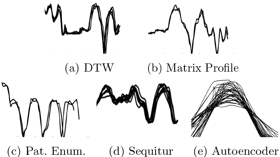

As mentioned in the introduction it is mandatory to have a pattern discovery algorithm that leads to results in an acceptable runtime. In Table 2 the runtime is given for the 1 mio. samples real life data set. Due to the fact, that data sets of vehicles are likely to be much longer than this, approaches like Matrix Profile or DTW are definitely not suitable to be applied to large datasets on a daily basis. CAE does need less than an hour, which may be acceptable with some more optimizations. Both discretization-based approaches run extremely fast, but especially the pattern enumeration subsequently requires some post processing to select relevant patterns.

6. Discussion

For the NN-based approach we utilized a Convolutional Autoencoder. We proposed adaptions concerning regularization terms and the architecture itself in order to enable it to find patterns in time series. We merged the advantages of 2D convolution with time series analysis by creating a new 2D time series representation. The time series is transformed into a 2D time series image by discretizing, slicing and one-hot-encoding to enable 2D convolution. In the end, using 2D instead of 1D convolution turned out to be essential for NN-based unsupervised pattern discovery. Beyond that, we developed a dynamic $L1$ regularization, which is independent from the number of weights in the convolutional filters. This ensures the influence of $L1$ regularization in the cost function to stay on a constant level, when varying the filter size. Furthermore, we proposed to include an entropy regularization into the cost function and compared it to the usage of Total Variation Distance regularization. Additionally, we applied a dropout layer to the network and enabled GPU computing. Each of these adaptions are necessary in order to make the Autoencoder competitive regarding nonlearning pattern discovery techniques.

In an extensive test we identified advantages and weaknesses of all approaches to especially rank the NN-based approach regarding nonlearning approaches. In general, discretization-based approaches have a high performance concerning runtime while the DTW-based approaches perform best regarding the quality of the results. The Matrix Profile can be classified as not suitable for our use cases due to the inability of time scaling and the unacceptable runtime. The Convolutional Autoencoder, including our adaptions, identifies patterns with a similar quality like the discretization-based approaches, but needs much more time. Nevertheless, the Convolutional Autoencoder can be considered as a valuable alternative because it automatically discovers the patterns that in total best cover the time series. Hence, it contains a functionality that needs to be additionally implemented when using one of the other approaches.

A major weakness of the Convolutional Autoencoder is the effort of parametrization and the parameter settings being far from universal. As we showed in this study, 14 parameters are need to be set carefully in order to get good results. We were able to reduce the effort of parametrization to just 6 parameters. The remaining 8 can be kept constant within one kind of data sets. Unfortunately, if it is applied to a completely new kind of pattern discovery use case all parameters need to be reconsidered. Hence, if the use case does not change fundamentally, the Convolutional Autoencode is a valuable alternative.

7. Conclusion and outlook

In this work we developed a new NN-based approach for unsupervised pattern discovery in time series, compared it to three nonlearning techniques and evaluated them concerning special requirements, that derive from automotive use cases. Even though NN-based approaches currently have major weaknesses regarding the task of pattern discovery, they are still interesting because of their ability to capture highly complex relations. Thus, it was shown that the Convolutional Autoencoder is able to discover patterns with a similar quality like discretization based approaches. Due to the highly dynamic developements regarding NNs we encourage everyone to also consider NN-based approaches. In future work the Convolutional Autoencoder will be extended to the multivariate discovery of patterns. Additionally it would be interesting to include varying filter lengths into one and the same Autoencoder to eliminate the necessity to run it multiple times. Furthermore, the usage of sparse Convolutional Autoencoders like in [37] offers the potential of runtime reduction. One major task is the robustness of parameter settings, when switching between time series of different origin, especially in case of real life data. Beyond that, the layer-wise increase of depth and the implementation of other unsupervised learning techniques (e.g. based on LSTMs) has to be evaluated.

Footnotes

These reference approaches are classified as nonlearning, because they do not apply neural-learning. We are aware that the reference approaches do also have some kind of learning procedure. For simplicity these approaches will be named as nonlearning.

Acknowledgments

We thank the anonymous reviewers for their valuable comments that led to a significant improvement of the manuscript. We thank Thomas Lehmann3

thomas.lehmann@ivi.fraunhofer.de, Fraunhofer IVI, Dresden, Germany.

and Dr. Ralf Bartholomäus4

⁴

ralf.bartholomäus@ivi.fraunhofer.de, Fraunhofer IVI, Dresden, Germany.

for the cooperation concerning the adaption and implementation of the DTW-based approach (Section 3.1). Furthermore we thank Jan Piewek

⁵

jan.piewek@volkswagen.de, Volkswagen AG, Wolfsburg, Germany.

for helpful ideas and discussions concerning the discretization-based approaches (Section 3.2).

References

Yeh

Kavantzas

Keogh

. Matrix Profile VI: Meaningful Multidimensional Motif Discovery. In: IEEE International Conference, 2017, pp. 565-574.

Lin

Oates

. Visualizing Variable-Length Time Series Motifs. In: Proceedings of the Twelfth SIAM International Conference on Data Mining, Anaheim, California, USA, 26-28 April 2012, pp. 895-906.

Noering

FKD

Jonas

Klawonn

. Assessment and Adaption of Pattern Discovery Approaches for Time Series Under the Requirement of Time Warping. In: Proceedings of 19th Intelligent Data Engineering and Automated Learning (IDEAL’13). vol. 11314 of LNCS. Springer International Publishing, 2018, pp. 285-296.

Rodríguez Lera

Martín

Matellán

. Neural networks for recognizing human activities in home-like environments. Integrated Computer-Aided Engineering. 2018; 26: 1-10.

Lara-Benítez

Carranza-García

García-Gutiérrez

Riquelme

. Asynchronous dual-pipeline deep learning framework for online data stream classification. Integrated Computer-Aided Engineering. 2020; 1: 1-19.

Molina-Cabello

Luque Baena

López-Rubio

Thurnhofer-Hemsi

. Vehicle type detection by ensembles of convolutional neural networks operating on super resolved images. Integrated Computer-Aided Engineering. 2018; 25: 1-13.

Macias-Garcia

Galeana-Perez

Medrano-Hermosillo

Bayro-Corrochano

. Multi-stage deep learning perception system for mobile robots. Integrated Computer-Aided Engineering, 2020; 8.

Rafiei

Adeli

. A New Neural Dynamic Classification Algorithm. IEEE Trans Neural Networks Learn Syst. 2017; 28(12): 3074-3083.

Ahmadlou

Adeli

. Enhanced probabilistic neural network with local decision circles: A robust classifier. Integr Comput Aided Eng. 2010; 17(3): 197-210.

10.

Alam

Siddique

Adeli

. A dynamic ensemble learning algorithm for neural networks. Neural Computing and Applications. 2020 Jun; 32(12): 8675-8690.

11.

Pereira

Piteri

de Souza

Papa

Adeli

. FEMa: a finite element machine for fast learning. Neural Comput Appl. 2020; 32(10): 6393-6404.

12.

Längkvist

Karlsson

Loutfi

. A review of unsupervised feature learning and deep learning for time-series modeling. Pattern Recognition Letters. 2014; 42: 11-24.

13.

Zhang

Yang

Tian

Zhang

. Unsupervised Feature Learning from Time Series. In: Proceedings of the Twenty-Fifth International Joint Conference on Artificial Intelligence. IJCAIâ€™16. AAAI Press; 2016, pp. 2322-2328.

14.

Zhuang

Huang

Cottrell

. Adversarial Dynamic Shapelet Networks, 2020.

15.

Keogh

. Time series shapelets: a new primitive for data mining, 2009, pp. 947-956.

16.

Benamara

Val-Calvo

Álvarez Sánchez

Díaz-Morcillo

Ferrández-Vicente

Fernández-Jover

, et al. Real-time facial expression recognition using smoothed deep neural network ensemble. Integrated Computer-Aided Engineering. 2020, 8.

17.

Bascol

Emonet

Fromont

Odobez

. Unsupervised Interpretable Pattern Discovery in Time Series Using Autoencoders. In: The joint IAPR International Workshops on Structural and Syntactic Pattern Recognition (SSPR 2016), pp. 427-438.

18.

Lee

Kim

. Convolutional Autoencoder Based Feature Extraction in Radar Data Analysis. In: 10th International Conference on Soft Computing and Intelligent Systems (SCIS) and 19th International Symposium on Advanced Intelligent Systems (ISIS), 2018, pp. 81-84.

19.

Radulovic

Kanjer

Plataniotis

. Discriminative Pattern Mining for Breast Cancer Histopathology Image Classification via Fully Convolutional Autoencoder. IEEE Access. 2019; 7: 36433-36445.

20.

Hoeppner

. Improving time series similarity measures by integrating preprocessing steps. In: Data Mining and Knowledge Discovery, 2017, pp. 851-878.

21.

Toyoda

Sakurai

Ishikawa

. Pattern discovery in data streams under the time warping distance. Very Large Data Bases. 2013; 22(3): 295-318.

22.

Jancovic

Köküer

Zakeri

Russel

. Unsupervised discovery of acoustic patterns in bird Vocalisations employing DTW and clustering. In: 21st European Signal Processing Conference, 2013, pp. 285-296.

23.

Lin

Keogh

Lonardi

Chiu

. A symbolic representation of time series, with implications for streaming algorithms. In: ACM SIGMOD Workshop on Research Issues in Data Mining and Knowledge Discovery (DMKD’03), 2003.

24.

Smith

Waterman

. Identification of common molecular subsequences. Journal of Molecular Biology. 1981, pp. 195-197.

25.

Nevill-Manning

Witten

. Identifying hierarchical structure in sequences: a linear time algorithm. Journal of Artificial Intelligence Research. 1997; 7: 67-82.

26.

Coquery

Jabbour

Sais

. A constraint programming approach for enumerating motifs in a sequence. In: International Workshop on Declarative Pattern Mining, 2011.

27.

Rajeb

Loukil

Hamadou

. On the enumeration of frequent patterns in sequences. In: The International Conference on Artificial Intelligence and Pattern Recognition, 2014.

28.

Fournier Viger

Lin

Gomariz

Gueniche

Soltani

Deng

, et al. The SPMF Open-Source Data Mining Library Version 2. vol. 9853; 2016, pp. 36-40.

29.

Yeh

Zhu

Ulanova

Begum

Ding

Dau

, et al. Matrix Profile I: All Pairs Similarity Joins for Time Series: A Unifying View That Includes Motifs, Discords and Shapelets, 2016, pp. 1317-1322.

30.

Madrid

Imani

Mercer

Zimmerman

Shakibay

Keogh

. Matrix Profile XX: Finding and Visualizing Time Series Motifs of All Lengths using the Matrix Profile. In: IEEE Big Knowledge 2019.

31.

Zhu

Zimmerman

Senobari

Yeh

Funning

Mueen

, et al. Matrix Profile II: Exploiting a Novel Algorithm and GPUs to Break the One Hundred Million Barrier for Time Series Motifs and Joins. In: IEEE International Conference on DataMining, 2016, pp. 739-748.

32.

Zhu

Yeh

Zimmerman

Kamgar

Keogh

. Matrix Profile XI: SCRIMP++: Time Series Motif Discovery at Interactive Speeds. In: IEEE International Conference on Data Mining, ICDM 2018, Singapore, November 17-20, 2018, pp. 837-846.

33.

Zimmerman

Kamgar

Senobari

Crites

Funning

Brisk

, et al. Matrix Profile XIV: Scaling Time Series Motif Discovery with GPUs to Break a Quintillion Pairwise Comparisons a Day and Beyond. In: Proceedings of the ACM Symposium on Cloud Computing, SoCC 2019, Santa Cruz, CA, USA, November 20-23, 2019; pp. 74-86.

34.

Linardi

Zhu

Palpanas

Keogh

. Matrix Profile X: VALMOD – Scalable Discovery of Variable-Length Motifs in Data Series. In: Proceedings of the 2018 International Conference on Management of Data, SIGMOD Conference 2018, Houston, TX, USA, June 10–15, 2018, pp. 1053-1066.

35.

Selesnick

. Total variation denoising (an MM algorithm). NYU Polytechnic School of Engineering Lecture Notes, 2012.

36.

Salvador

Chan

. FastDTW: toward accurate dynamic time warping in linear time and space. In: KDD Workshop on Mining Temporal and Sequential Data, 2004.

37.

Luo

Yang

Zhang

. Convolutional Sparse Autoencoders for Image Classification. IEEE Transactions on Neural Networks and Learning Systems. 2018; 29(7): 3289-3294.

Pattern discovery in time series using autoencoder in comparison to nonlearning approaches

Abstract

Keywords

1. Introduction

1.1 Motivation

1.2 Related work

1.3 Purpose and structure

2. NN-based approach for pattern discovery

2.1 Convolutional autoencoder

3.1 DTW-based

3.2.2 Adapted Sequitur algorithm

4.1 Time series test data creation

4.2 Pattern evaluation

5.1 Comparison of best results

Table 1 Overview of varied parameters for the experiments of CAE

5.4 Evaluation of discretization-based approaches

5.6 Application to real Life data set

Table 2 Exemplary results for real data set

7. Conclusion and outlook

Footnotes

Acknowledgments

References

Table 1
Overview of varied parameters for the experiments of CAE

Table 2
Exemplary results for real data set