A methodology using classification for traffic prediction: Featuring the impact of COVID-19

Abstract

This paper presents a novel methodology using classification for day-ahead traffic prediction. It addresses the research question whether traffic state can be forecasted based on meteorological conditions, seasonality, and time intervals, as well as COVID-19 related restrictions. We propose reliable models utilizing smaller data partitions. Apart from feature selection, we incorporate new features related to movement restrictions due to COVID-19, forming a novel data model. Our methodology explores the desired training subset. Results showed that various models can be developed, with varying levels of success. The best outcome was achieved when factoring in all relevant features and training on a proposed subset. Accuracy improved significantly compared to previously published work.

Keywords

Traffic prediction classification data mining smart cities COVID-19

1. Introduction

The deployment of modern cities increasingly gains attention, as large urban centers present numerous challenges for citizens over time. Traffic is a stressful and time-consuming factor affecting citizens. Lately, many local authorities attempt to design and create smart infrastructures and tools to collect data and utilize prediction models for better decision making and citizen support. Such data are often derived from sensors collecting information about Points Of Interest (POIs) in real time. Data mining techniques and algorithms can then support getting useful insights into the problem, whilst forming appropriate strategies to counter it.

This work proposes a methodology for day ahead traffic prediction utilizing feature engineering on sensor and weather data, and classification methods, exploring the impact of local lockdowns imposed due to the recent pandemic. It analyzes various data engineering approaches applied to data associated with weather conditions, seasonality, and the impact of COVID-19 related restrictions.

The proposed models utilize weather data collected from sensors located in Athens and Thessaloniki, Greece. This work extends our research, which utilized three time slots (Morning, Afternoon, Evening) over subsets of trimesters throughout a range of 6 months [1]. It expands the analysis by investigating the impact of a fourth time slot, namely Noon. In addition, 4-month periods of time, extended with the introduction of new features, are also tested and verified.

Moreover, we focus on identifying a training data subset that could outperform the accuracy of our model on the whole available dataset. Indeed, the subset of data collected throughout the lockdown period introduced by Greek government (168 days), outperformed all the rest when using binary classification.

We also analyze how COVID-19 impacted traffic loads, being incorporated as a factor supplementary to weather conditions. The outbreak of COVID-19 has affected everyday life of citizens, as several local authorities have introduced strict lockdowns. In addition, promotion of remote working has reduced the number of citizens who travel around cities, while typical rush hours tend to fade away. Different counties and cities as well as communities, tend to adapt differently to the fast spread of COVID-19 and subsequent restrictions. The incorporation of features related to movement restrictions, led to identifying abnormal traffic conditions and formed a successful novel data model.

Additionally, it contributes to the understanding of how major unexpected conditions can modify traffic loads on a temporary/semi-permanent basis and whether models trained on regular conditions can adapt or not.

This work differs from standard approaches for traffic prediction in several ways, mainly associated with the methodology and the ultimate aim. To the best of our knowledge, the transformation of the problem into classification and the inclusion of movement restriction parameters has not been used so far, for predicting day-ahead traffic conditions. Our contribution can assist predictions in the day-ahead scenario.

Our focus is also on investigating whether we can build reliable models by utilizing smaller partitions of data. In other words, our methodology attempts to investigate the optimal degree of data aggregation, which is an open research question [2].

The remaining of the paper is structured as follows: Section 2 provides background information and reviews the literature. Section 3 presents the methodology we followed for traffic prediction, including data selection. Section 4 presents experimental results. Section 5 discusses and evaluates research findings, while Section 6 concludes the paper with suggestions for future work.

2. Literature review

Traffic prediction is not a new subject; there are numerous scientific efforts that perform either classification [3, 4, 5, 6, 7, 8] or regression tasks [9, 10, 11, 12]. Traffic prediction is considered as short-term for time periods of 5–30 min and as long-term for any period from a few hours to 1 day or even more. Most efforts attempt short-term predictions [11, 12, 13, 14], while only a few try to predict long-term traffic based on weather data [15, 16, 17].

Recent research focused on the impact of COVID-19 on traffic prediction. In [18] a new human mobility flow clustering model was developed and compared in the Milwaukee and Dane Counties. O-D flow data were utilized and considered a significant input to the transportation analysis. The sensitivity of their clustering methods was tested on data regarding different periods. The investigation between COVID-19 spread and traffic flow, reveals that although traffic restrictions were active, the infection rate was still high.

The unprecedented restrictions have caused a status of abnormality in the way several city-problems are being approached. Noise-emission is a close-related problem with traffic load, as vehicles represent a great factor in the equation.

A very interesting analysis of urban traffic volumes in Rome [19] highlights the significant drop of traffic (and noise) through the utilization of Floating Car Data (FCD) collected by anonymous vehicles. The drop based on the baseline load was steadily above 50% for the main lockdown period and a second phase of gradually lifted measures did not significantly affect road networks. The specific analysis focused on the typical rush hours between 7–10 am. Thus, it is clear that already developed models, trained on data regarding periods of normality are not expected to be reliable on predictions during state-designated restrictions. Currently data related to the COVID-19 spread are available on numerous dashboards [20] and should be carefully taken into consideration, while training predicting models.

Another approach on building applications to predict traffic demand is the utilization of wavelet analysis. Adeli et al. proposed a mesoscopic-wavelet model for simulating traffic flow patterns in a freeway and identifying congestion characteristics [21]. Additionally, a wavelet packet-autocorrelation method enabled noise removal and singularity identification [22], while a dynamic recurrent wavelet Neural Network (NN) model combined self-similar, singular, and fractal properties identified in the traffic flow [23].

Furthermore, a NN-wavelet microsimulation model was applied to estimate delay and queue length in work zones. This model could capture the dynamics of a single vehicle in changing traffic flow conditions [24]. Dunne et al. utilized neuro-wavelet models along with the rain expectation in the next hour [25].

Nejad et al. examined the power of decision trees for classifying traffic loads on three levels, based only on time and temperature [3]. Results were positive and motivated our work. Xu et al. compared CART with k-NN and a direct Kalman Filter [26].

Moreover, Wang et al. proposed the use of volume and occupancy data [4]. Such data, as well as speed, can be obtained by loop detectors, which are sensors buried underneath highways, estimating traffic by observing information related to vehicles passing above them. Loop detectors along with rain predictions were also used to predict crashes [27].

Tree-based algorithms are widely used and justified. However, even more sophisticated algorithms were used, such as Support Vector Machines (SVMs) [5] and NNs [28]. A novel hybrid method for short-term traffic prediction under both typical and atypical traffic conditions was introduced by Theodorou et al. using an SVM based model that identifies atypical conditions [10], applying ARIMA or k-NN regression to identify typical or atypical conditions, respectively.

In addition to [4], Liu et al. introduced three binary variables, other than weather conditions, for holiday, special conditions, and quality of roads [16]. Abnormal conditions have a negative impact on such models; for instance, when attempting to estimate the traffic flow based on Expressway Operating Vehicle [11]. The lockdown imposed by the pandemic of COVID-19 is an example of long-lasting atypical conditions.

Qiao et al. presented a travel time prediction model with weather information such as precipitation type, visibility and wind speed from a 10-month period. For normal weather conditions, ARIMA and KNN are proposed, while under extreme weather a KNN model-based with a trend adjustment feature performs better [13]. In addition, other research on long-term traffic flow prediction included weather data such as temperature, solar radiation, wind speed, rainfall, pressure, humidity and ultraviolet radiation [17].

Another significant decision on such predictions relates to the actual day of the week. Weekdays tend to have different characteristics from weekends and should be carefully tested [12, 29]. Finally, most scenarios regard short-time prediction, meaning minutes to hours ahead.

Especially, for the case of Thessaloniki Mystakidis et al. investigated the traffic system and suggested that the size and the quality of the dataset affects the model’s accuracy, and a Decision Tree Classifier was identified as the best performer [6].

A methodology for spatio-temporal predictions of traffic volumes and greenhouse emissions on road segments was developed [30]. Respectively, a 3D convolutional NN [31] and a fully convolutional model [32] were developed to predict traffic by extracting spatial-temporal characteristics. According to Zhang et al. spatio-temporal characteristics are extracted with computational complexity linearly related to the number of road segments [14].

Ferreira et al. have developed a model that supports spatio-temporal queries on taxi trips in New-York City, detects patterns and creates visual representations of the traffic system. Moreover, they created pickup and drop-off clusters, studied traffic flow to main hubs, such as train stations and airports, and investigated how the state changes over time [33]. Another research by Antoniou et al. on traffic data from sensors, proposed that a lower number of clusters related to traffic states leads to better performance [34].

Hashemi et al. employed classification techniques to predict the future traffic state. The target variable was the Level Of Service (LOS) in short time intervals; it was better predicted by Classification Tree and Random Forest [7]. Another purpose of this paper was to extract if-then rules, used for studying traffic patterns. Extracting these patterns and understanding the traffic system parameters, such as speed, flow, and travel time, could benefit traffic management. Similar research aimed at predicting traffic congestion using association rules to achieve higher accuracy in classification problems, considering the traffic environment [35].

Pan et al. proposed a feature selection model to investigate the impact of traffic incidents. According to this study, it is urgent to include non-recurring incidents, such as accidents, music concerts, road reconstruction, because these events are possibly related to traffic jams. Considering all these factors, their prediction model combines historical data and event information, and outperforms well known algorithms in terms of accuracy, for different traffic conditions [9].

Gecchele et al. presented a comparison between various clustering methods to estimate the Annual Average Daily Traffic (AADT). Results have shown that model-based clustering methods, such as the Variable Equal Identity (VEI) model, achieve marginally better results than hierarchical and partitioning methods. This work suggests that traffic prediction is more demanding on weekdays as well as during the summer and depends on vehicle-type for trucks [36].

Data mining techniques, such as K-means, were applied to generate patterns based on temporal and spatial characteristics [37]. Results indicate that peak hours are identified between 7:45 and 8:45 in the morning, as well as between 17:15 and 18:15 on weekdays. Another study proposes a scalable distributed stream mining system for highway traffic data, which can perform traffic analysis and detect real time abnormal events, traffic congestion and predict flow speed [8].

Vlahogianni et al. established that further research is needed to ascertain the optimal degree of data aggregation [2]. Another challenge mentioned was the need for prediction models robust to longer term changes (e.g. lockdown) in traffic conditions. Further review of the literature verified their suggestions, since there is a significant research gap regarding long-term (day-ahead, week-ahead) traffic prediction during long-lasting events that affect traffic. Motivated by this, and in the light of movement restrictions introduced, we decided to highlight this special period of lockdown due to its potentially long term implications.

3. Traffic prediction methodology

Most studies focus on either predicting traffic loads for a certain time interval or selecting the optimal route based on real-time adaptations. Traffic is affected by various factors, only some being predictable. As mentioned in Section 2, traffic is directly affected by weather conditions, however the scale differs across cities, cultures and climate zones. This section presents the problem we address and describes our methodology, as well as the data collected and the preprocessing conducted, prior to experimentation, presented in Section 4.

3.1 Problem definition and methodology

This section tests our intuition about traffic prediction presented above. Special events can shortly disrupt normal traffic in specific areas, while seasonality and weather conditions can affect traffic on a larger scale. Based on that, weather data were collected from sensors installed around carefully chosen city spots, for predicting the day-ahead traffic state.

The approach followed, besides examining traffic predictability based on weather data, also aims to clarify differences among the two cities, Athens and Thessaloniki. We created two new features that describe “abnormal” or atypical conditions throughout the year, one for the separation of weekdays from weekends and one applying to movement restrictions. Moreover, a series of experiments were conducted regarding different monthly periods, serving the objective to understand which months contribute positively to the deployment of such models. The approach we followed is further elaborated in Section 4.

In addition to the main problem we addressed, the outbreak of COVID-19 added a new dimension to our research. Two questions were integrated into the problem definition: The first question was: “in what way did lockdown restrictions imposed because of COVID-19 affect traffic?” The second question was: “in what way is a model for traffic prediction affected by emergency situations like the COVID-19 pandemic?” Following this, we focused on creating another subset of data related to the lockdown period and examined the new model developed for it.

3.2 Data description

Our data source was ppcity.io, an open integrated system of platforms, which promotes contextual engineering and citizen involvement in decision making and life quality improvement. Multiple environmental, geospatial, and traffic data have been integrated into ppCity platforms. They are collected from various sources and serve our analysis purposes.

We focused on data extracted from sensors located at central points in Athens and Thessaloniki, Greece. These two urban centers host almost half the Greek population. In general, there are numerous city spots in both cities, where the environmental and traffic conditions are measured. Initially, locations were chosen according to data available regarding traffic and weather conditions. The focus of our attention was on 26 reliable spots that produce data, i.e. sensors with the wider range of recording and most compact flow of data.

Figure 1.

Jam Factor during 07.2019–08.2020.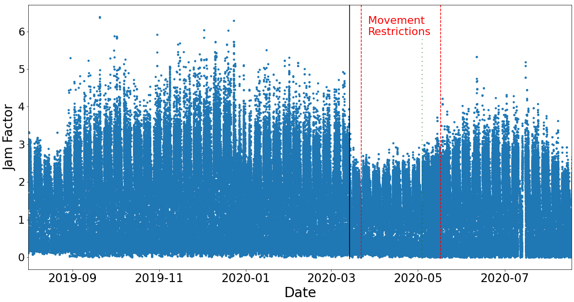

Figure 2.

Average Jam Factor per day.

Weather related attributes we used for our analysis involved the following: Humidity, Pressure, Temperature, Wind Direction, Wind Speed and Ultraviolet Radiation (UV). The target variable (traffic load), named Jam Factor, represents quality of travel. It ranges from 0 to 10, where 0 describes a completely empty road and 10 stopped traffic flow. The exact formula for computing the Jam Factor is not public. However it is known that it depends on the expected default travel speed (base speed in meters per second), the actual travel speed (traffic speed in meters per second), the road type, and other conditions (see Documentation Here [38]). The Jam Factor has also been used in traffic applications, such as vehicle energy use prediction [39], parking availability [40] and propagation of traffic congestion [41]. The dataset consists of 233 K records, which were collected between 01.08.19 and 31.08.20, including time periods with movement and transportation restrictions due to COVID-19.

The Greek government took the following measures to hinder the spread of COVID-19:

•

On March 23, 2020, they implemented a general lockdown and introduced an SMS based system to provide movement permits within regional units.

•

On May 4, 2020, they abolished the SMS system, but preserved regional restrictions regarding transportation.

•

On May 18, 2020, they permitted free and unconditional movement and transportation.

Figure 3.

Jam Factor hourly average.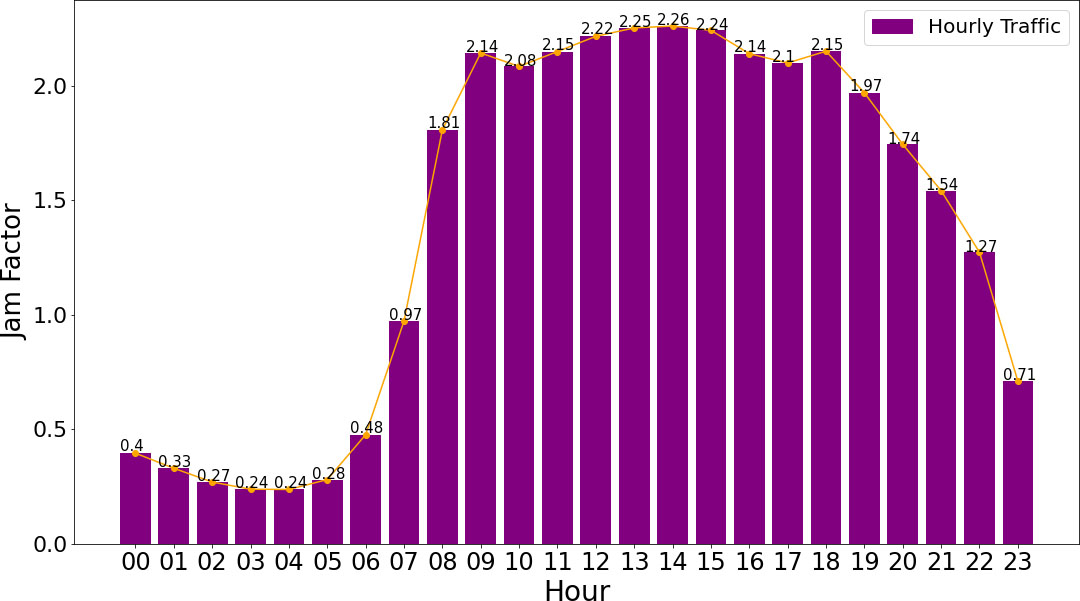

Consequently, based on movement and transportation restrictions imposed by the Greek government due to COVID-19, we introduced a new feature, named “status”, and defined three time periods:

•

August 1, 2019, to March 22, 2020, the pre-lockdown period, with unrestricted transportation.

•

March 23, 2020, to May 17, 2020, the lockdown period, with restrictions on transportation.

•

May 18, 2020, to August 31, 2020, the post-lockdown period, with unrestricted transportation.

The aforementioned information is depicted in Fig. 1. The red (dashed) lines signify the beginning and the end of the government restriction measures. It is obvious that restrictions and public concerns over COVID-19 had a significant impact on the Jam Factor. It is also important to mention that there is a remarkable drop in the Jam Factor a few days before the implementation of the movement and transportation restrictions. This can be explained by the fact that coffee shops, bars and shopping centers were forced to close on March 14, 2020, exactly where the black (solid) line is. We can additionally observe that the gradual increase in the Jam Factor after the COVID-19 period, actually begins at the green (dotted) line, which signifies the day that the SMS system was abolished by the government (May 4, 2020), and movement restrictions were relaxed.

Another special feature that was incorporated to our research was derived from the segregation of the days examined into weekdays and weekends. Figure 2 illustrates a significant drop of the Jam Factor during weekends, which deepens on Sundays. Thus, a new Boolean attribute was created, to examine the effect that weekends have on predicting the Jam Factor.

Those two features were implemented either individually or conjointly, contributed to model evolution and improved accuracy. Their effect is further analyzed and detailed in Section 4.

Figure 4.

Sensor location in Thessaloniki (left) and Athens (right).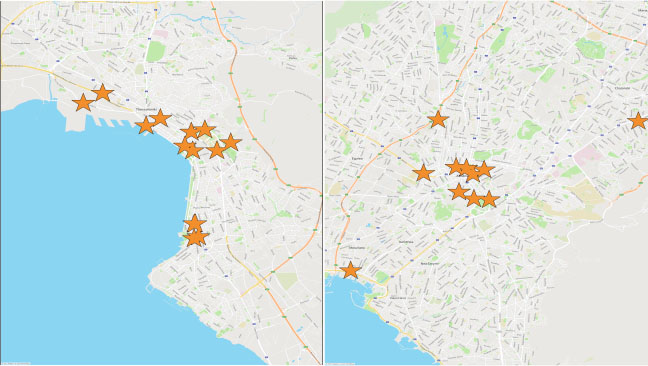

3.3 Data processing

The way the data were processed is conceptually straightforward. Regarding the data structure, three distinct time intervals within a day were originally defined and their predictability was examined [1]. Initially the focus was set on specific hours, which were recognized as the time intervals when people drive to or depart from their jobs, and the time interval that they usually go out for entertainment. The first interval, named Morning, includes data from sensors between 07:00 and 10:00. The second one, named Afternoon, includes data between 15:00 and 18:00 and the last one, named Evening, includes data between 19:00 and 22:00.

Therefore, the average value for the given data was computed. For example, if a sensor captures information every hour (e.g. at 07:10, 08:10, 09:10 etc.), the average value for each weather metric and the traffic load for that specific interval was computed. The rationale for this aggregation emerges from the fact that we try to follow the format of weather predictions. Typically, weather forecasting is provided in similar 3 or 4-hour intervals by the majority of meteorological institutes. Since our data reflect weather conditions we chose to aggregate as described.

In our earlier work [1], the above strategy resulted in creating three different datasets originating from a 6-month period. Fortunately, the quality of the dataset was high, missing values being scarce. It is worth noting that the averaging strategy implemented does not replace missing values. If there is a missing value in weather metrics, averaging is performed using the remaining two available values, instead of averaging and labeling three values.

To extend this work, we added a new time interval, named Noon, that includes data from sensors between 12:00 and 15:00, as it relates to school runs and shops, as well as public organizations closed for the afternoon break. This time interval was deemed to be important for our research.

As seen in Fig. 3, interestingly, the Jam Factor during Noon is slightly higher than any other time within the day. The time periods when people drive to their jobs and when they drive back home are generally considered as rush hour. Usually rush hours are before 12:00 and after 15:00. However, in big cities like Athens and Thessaloniki, there is a high volume of traffic even during noon, when people need to move through the city for tasks like school runs, shopping, business meetings, urban freight transport, as well as returning from work which stops around 3 p.m.. Thus, the time interval called Noon, can also be regarded as rush hour.

For our earlier work we used data derived from 10 sensors for only 6 months [1]. This time we collected data from 26 sensors over 13 months maintaining high quality consistently.

Moreover, the initial imbalance between the sensors located in Thessaloniki and Athens was addressed. Initially, 8 sensors were in Athens and 2 in Thessaloniki. This time we collected data from 10 sensors in Athens and 16 in Thessaloniki. Their location is depicted in Fig. 4. With this distribution of sensors, a straightforward comparison of the model’s reproducibility is now possible. Thus, result credibility has been enhanced.

Additionally, recursive feature elimination was implemented to select the optimal subset of features. The least important feature was wind direction and was removed. According to Fig. 5, the “weekends” feature demonstrates the highest importance score by far. Next come “uv” and “status” with equal high importance scores. The remaining features, such as temperature and atmospheric pressure, refer to weather conditions. These features are related to weather phenomena that strongly affect traffic. For instance, rain and snow often limit movement and cause traffic congestion.

Figure 5.

Feature importance using recursive feature elimination.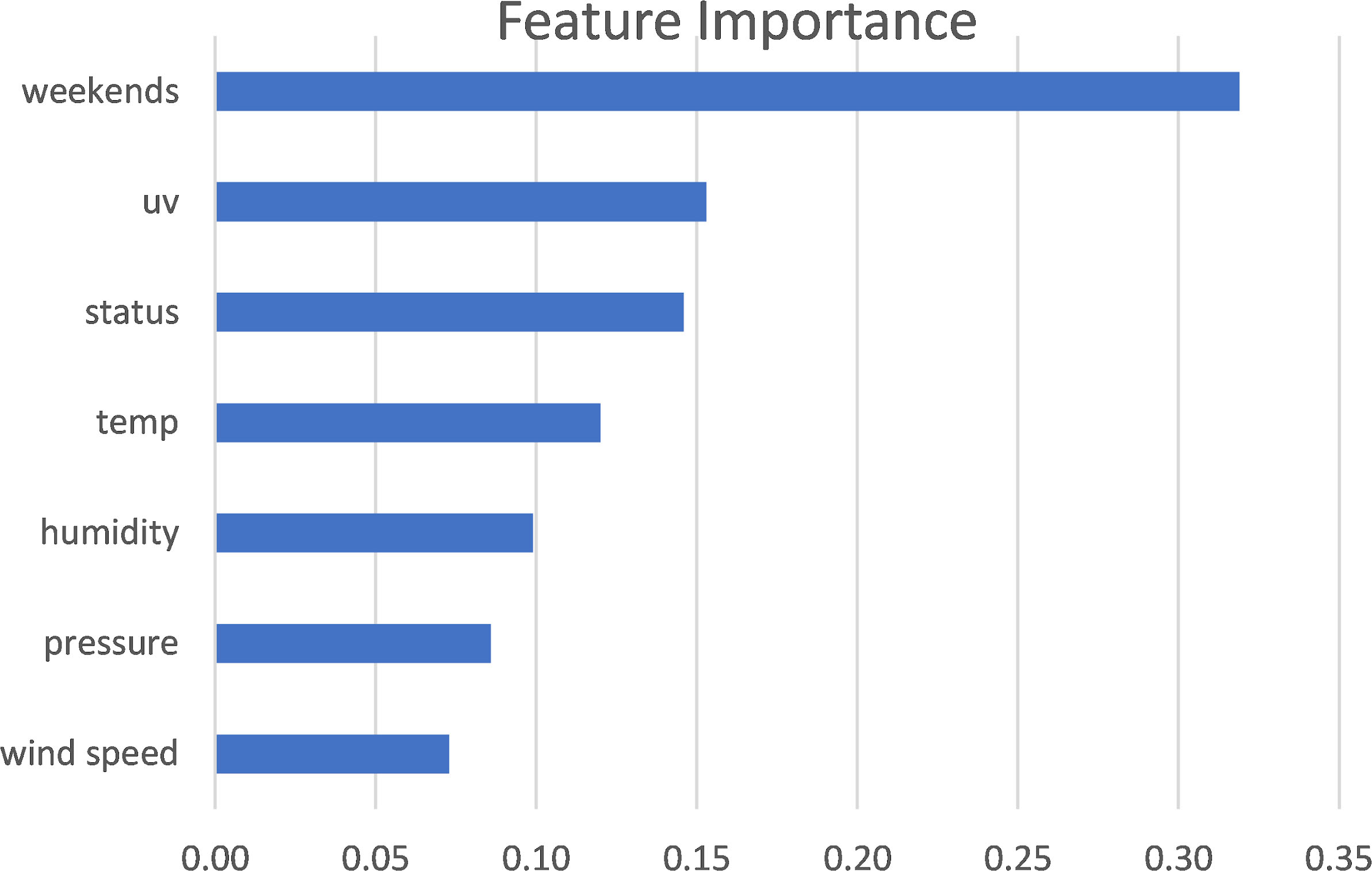

Reformulating the problem from one requiring regression to one suitable for classification by categorizing the target variable into two and later into three classes, was another key decision. Instead of using regression techniques to predict the exact Jam Factor value, we opted to use classification, as our broader motivation was to identify factors that affect day-ahead predictions. A regression output is not considered as a fully interpretable value for citizens and the standard deviation is admittedly low ( $s=$ 1 during 24-hour and $s=$ 0.8 for 07:00–22:00), while the real range of the Jam Factor equals 6.38. The binary and ternary classification scenarios are introduced, since the range and standard deviation are quite small and more typical numbers of classes (for example 5 or 10) would result in highly imbalanced datasets. Those were the main reasons behind our decision to transform the problem into one requiring long-term classification. Thus, the whole process could also be automated. Forecasting Jam Factor fluctuations has a different purpose from building a short-term model that focuses on the exact Jam Factor value.

An investigation was conducted on how effective the model is for each set of parameters and which reasons lead to differentiation in accuracy. Therefore, the model was initially transformed into a binary one. The split point was the median value for each dataset, aiming at a fully balanced task, which would grant safer conclusions. The two initial labels were “High” and “Low”, with regards to the Jam Factor. In a different set of experiments, the target variable was split into three categories of equal size (namely, “High”, “Medium” and “Low”), following the same splitting strategy. The metric used for evaluation was accuracy since classes are balanced and of equal interest. Its mathematical representation is shown below:

$\displaystyle\text{Accuracy}=\frac{\textit{TP}+\textit{TN}}{\textit{TP}+% \textit{TN}+\textit{FP}+\textit{FN}}$ (1)

where TP denotes true positive, TN denotes true negative, FP denotes false positive, and FN denotes false negative.

Figure 6.

Comparing logistic regression and random forest classifiers in 2-classes and 3-classes.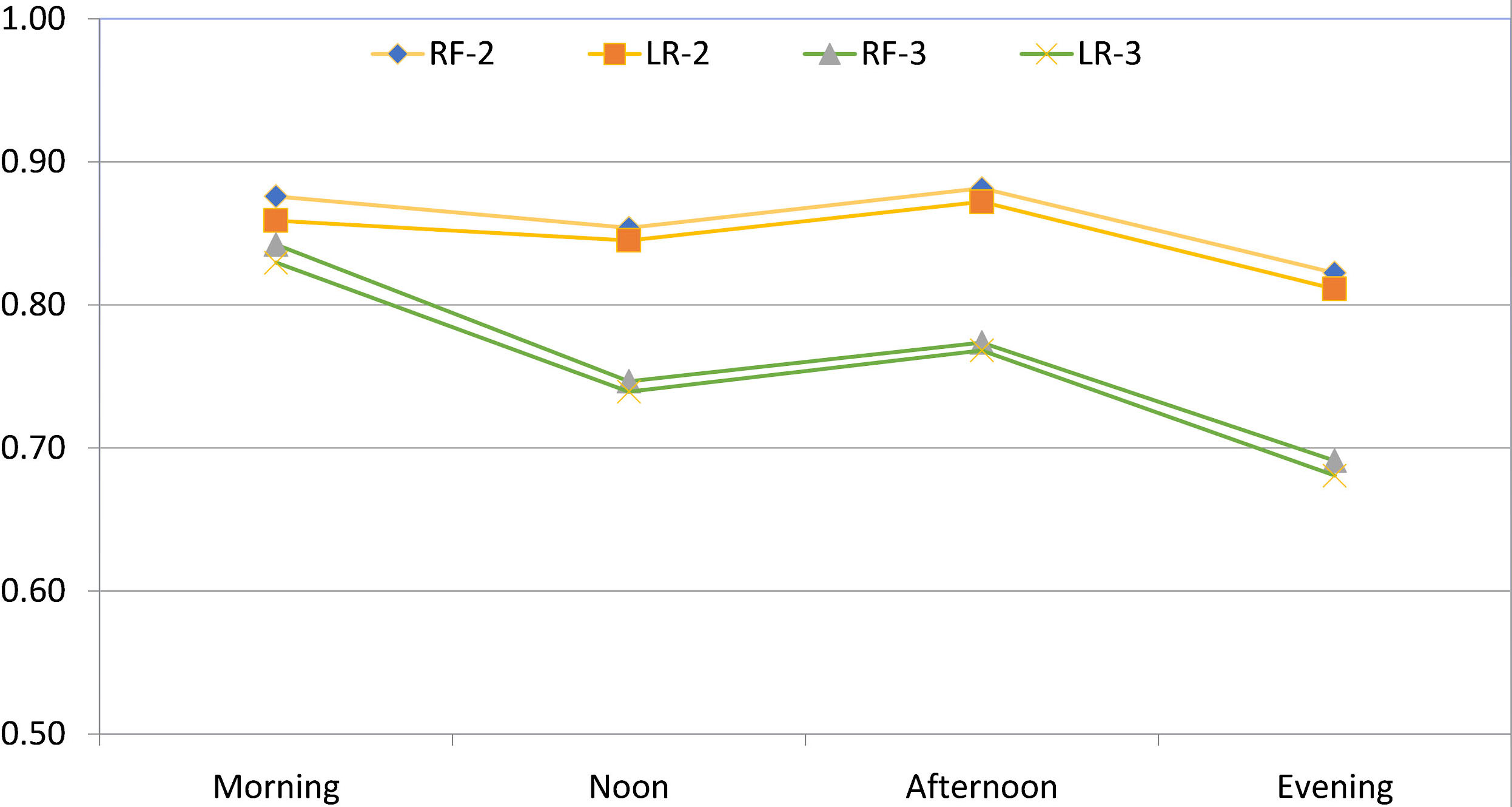

Through the experiments, it was ascertained that the two models display almost identical trends, but the 2-classes model produced, as expected, consistently better results than the 3-classes model, in terms of accuracy. Therefore, our experiments emphasized on using only two classes, namely “High” and “Low”.

After training the model, two types of model evaluation were used. One involved using a test set, containing 20% of the available, and another using a validation set. Both evaluation types produced identical results with high accuracy. The results presented in Section 4 pertain to the type using the validation set, as it emerged after a 10-fold cross validation.

Finally, apart from splitting the time based on COVID-19 related restrictions, seasonal based segregations were also performed. Models based on both 3-month and 4-month intervals were used and their results were compared with the results from the whole dataset. Interesting conclusions were extracted and are discussed in Section 5.

4. Experiments

This section presents experiments we conducted on our data. We start by briefly presenting our baseline, results reported in our earlier work [1]. We then provide results produced by our extended model, featuring improvements, such as the introduction of an attribute related to the type of day (weekday vs. weekend), the type of period related to COVID-19 (pre-, during, and post-lockdown) as well as their combination. We also present experimental results related to 3- or 4-month splits of the data. We conclude with a comparison between results for Athens and Thessaloniki.

4.1 Baseline

As described in Section 3 both types of generalization (test set and validation set) and both splits into 2 or 3 classes have insignificant variation and almost identical trends. Using the validation set and test set display minor differences, with the validation set producing slightly better results in terms of accuracy. It was established that the model constructed with 2 classes for the target variable outperforms the 3-classes model. Two classifiers were used: Random Forest and Logistic Regression. Grid search was executed for both, in order to specify the optimal parameters of each given model. Other classifiers were also tested, namely SVM, MLP, C4.5 and K-NN, without providing any significant variation on results. We present only these which are more stable and better.

Figure 7.

Model evolution featuring all time intervals.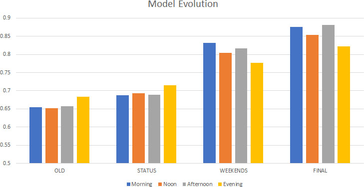

Figure 6 shows the accuracy achieved by Random Forest (RF-2, RF-3) and Logistic Regression (LR-2, LR-3) for the 2 and 3 class problems, respectively, with RF-2 being the best option followed by LR-2. For the 2-classes the model consistently achieved accuracy over 80%, with best results for Afternoon, while the 3-classes fared better in the Morning. Random Forest with 10-fold cross-validation achieved slightly better results than Logistic Regression. The trade-off between them is that Random Forest was 10 times slower than Logistic Regression. Random Forest was chosen due to its higher accuracy.

Thus, all remaining figures in the main body of this paper refer to results achieved using a validation set, for models trained with Random Forest and for target attribute with two classes. All figures that illustrate the results for three classes are available in Appendices A, C, D, respectively.

The original model [1] was not evaluated on predicting traffic congestion during special circumstances, such as the COVID-19 pandemic, and its accuracy fluctuated around 64%, as can be seen in the first set of four bars, labeled “OLD” in Fig. 7.

4.2 Model evolution

With the incorporation of the feature “status”, related to the lockdown due to COVID-19 (having three distinct values: pre-lockdown, lockdown, post-lockdown) into the original model, a slight improvement was observed, achieving accuracy close to 67% and over 70% for the Evening time interval. This can be observed in the second set of four bars labeled “STATUS” in Fig. 7.

Moreover, with the incorporation into the original model of the feature “weekends”, which categorizes days into weekdays and weekends, the new model achieves significant higher accuracy, even above 80% for Morning, as can be seen in the third set of four bars labeled “WEEKENDS”, in Fig. 7.

Finally, both these features, i.e. status and weekends are used conjointly to form the final model, illustrated by the fourth set of four bars in Fig. 7, labeled “FINAL”. Compared to the original approach, an undoubted improvement was achieved on accuracy, which increased to over 80% for all periods and approximated 90% for certain day intervals. Additionally, it is worth mentioning that the feature “status” contributes more to the classification task when combined with the feature “weekends” rather than merely added to the original model. Adding “weekends” actually offered higher improvement than that introducing “status”.

Another observation derived from Fig. 7 is that the two new features, namely “status” and “weekends”, have a different impact on each time interval. In particular, “status” has a homogenous impact on each time interval, by slightly improving accuracy ( $\sim$ 4%). On the other hand, the feature “weekends” seems to affect evening time intervals less than it affects the other three. It is observed that the Evening time interval has the best accuracy (68%) in the original model but has the worst accuracy (78%) when the feature “weekends” is incorporated into the model.

One possible explanation for that observation lies in the fact that evenings’ traffic congestion is related to transportation for recreation rather than for business purposes. Since weekends are rest days, it is normal for traffic congestion to be reduced during morning, noon and afternoon on those days, but this does not reflect the evening traffic loads. Therefore, while the prediction about the other three time intervals is heavily affected by the feature “weekends”, this is not the case about the Evening time interval.

This assumption is confirmed by Fig. 8, where it is obvious that, regarding the Jam Factor, the difference between weekdays and weekends is significantly lower during the evenings (19:00–22:00) than any other time interval.

Figure 8.

Average Hourly Jam Factor on weekdays vs. weekends.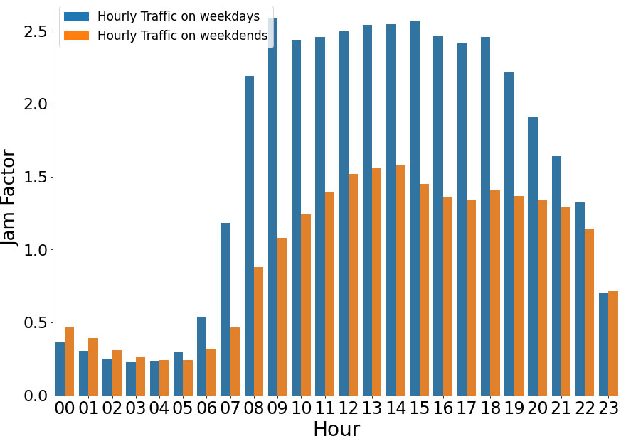

Figure 9.

Accuracy for 3-month periods and 2-classes.

Figure 10.

Performance in 4-month periods for 2-classes.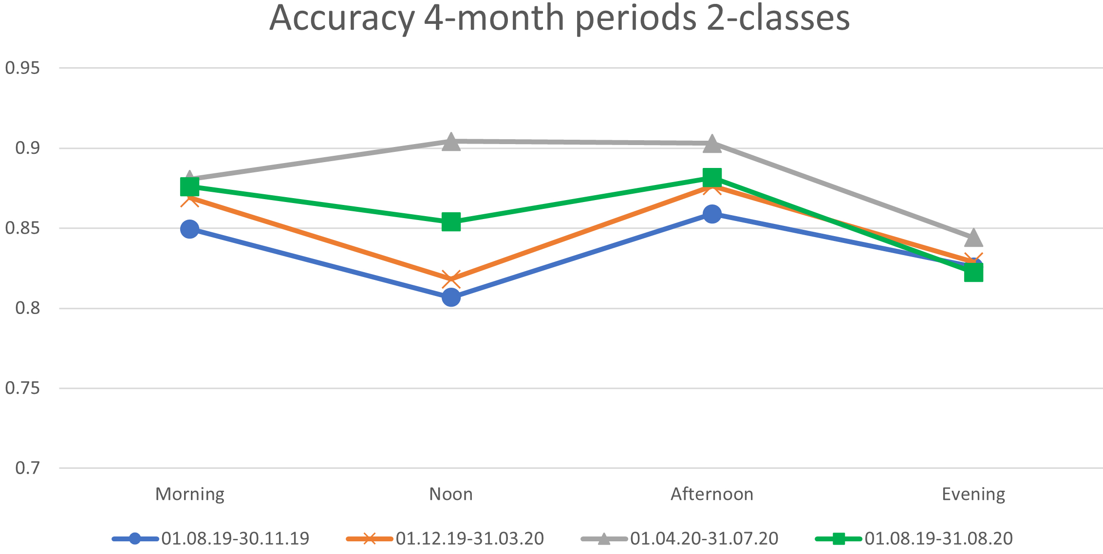

4.3 3-month split

By examining the dataset segregated using 3-month periods, it emerges that on average Morning (85%) and Afternoon (86%) are more predictable intervals than Noon (83%) and Evening (82%). As depicted in Fig. 9, the model trained on the whole dataset performs better (86%) than the other splits except for one: the best performing (87%) training period (01.05.20–31.07.20) contains both movement restrictions and free movement, which seems to be a key factor in data selection.

4.4 4-month split

The model is also trained and tested based on 4-month periods and compared to the training case of the whole dataset. The 3rd 4-month split (01.04.20–31.07.20) outperforms (88%) all others for every time slot. Observing Fig. 10 and comparing it to Fig. 9, the same patterns emerge as in the case of 3-month periods. For instance, the model performs on average better in the Morning (87%) and in the Afternoon (88%). The model trained with the whole dataset (01.08.19–31.08.20) achieves higher accuracy (86%) than the first two 4-months intervals (84%–83%) but is being outperformed (88%) by the last one (01.04.20–31.07.20). This remark also applies to Fig. 10.

It seems that a range containing both normal and special (COVID-19) traffic conditions is an optimal training period for the model. Moreover, since in this case there is a subset that outperforms (88%) the whole dataset (86%), we assume that it is recommended to include normal and special traffic conditions to our model. In any case, more data records do not guarantee higher accuracy.

Figure 11.

Accuracy comparison related to the lockdown.

Figure 12.

Accuracy comparison related to lockdown periods, featuring all time intervals.

4.5 COVID-19

It has already been mentioned that the Jam Factor and our predictions were influenced by the outbreak of COVID-19 (see Appendix B). To investigate that influence, the dataset was initially split into three periods of equal size of 56 days (pre-lockdown, lockdown, post-lockdown) and the results were compared with those for the whole dataset. Later, we merged those intervals and added one more time period, from 27.01.2020 to 12.07.2020 (168 days), which proved to be revealing. Results are presented in Fig. 11, after aggregating sensor outcomes for every time interval during the day.

Lockdown and post-lockdown periods turned out to be the most difficult to predict (76% and 75%), demonstrating the unexpected changes COVID-19 has caused to every-day life. The pre-lockdown split was the easiest to predict (84%). As previously exhibited, in pre-lockdown days, traffic conditions were normal. Afterwards, traffic dropped during the lockdown, and in post-lockdown days, rose but not up to normal levels. Subsequently, we assume that accuracy is affected by traffic conditions (i.e. movement restrictions) and that it is easier to predict traffic during normal traffic conditions.

Figure 13.

Average Jam Factor in Athens and Thessaloniki during 07.2019–08.2020.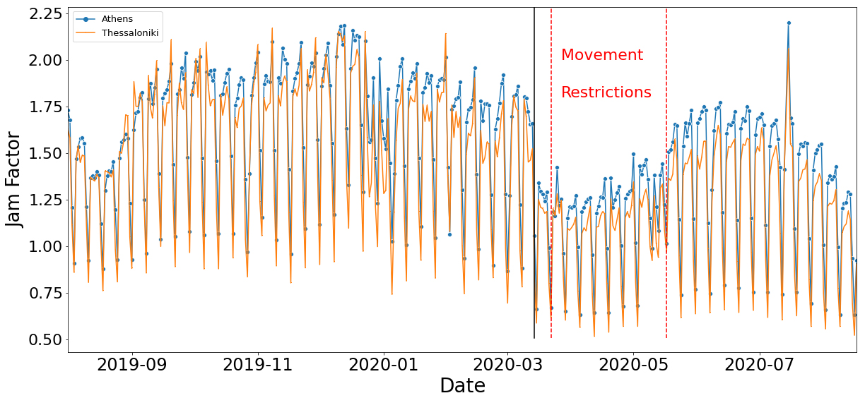

Figure 14.

Average Jam Factor in Athens and Thessaloniki before, during and after the lockdown.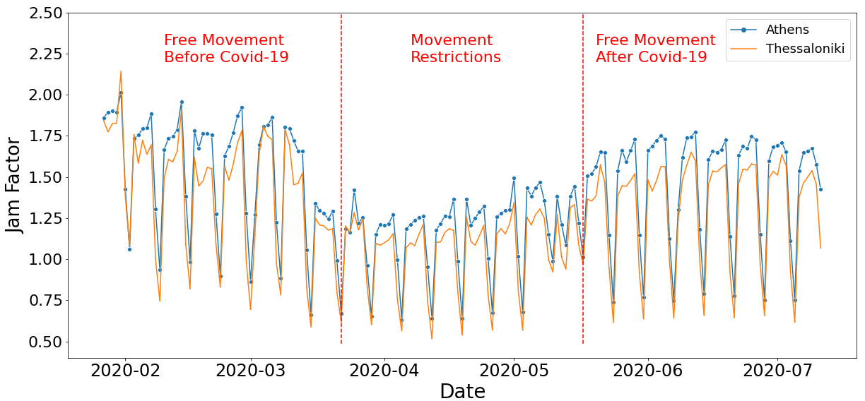

Interestingly, the model trained on the whole dataset produced better results (86%) than pre-lockdown, lockdown and post-lockdown periods, but “pre_until_post” outperformed (88%) all of them. In that case, the model trained from 27.01.2020 until 12.07.2020 achieved the highest performance with accuracy close to 90% (Morning, Afternoon). This can be explained by the fact that the feature “status”, which is one of the most important features of the model, during this period takes exactly an equal number of values from each category.

Consequently, there is a perfect balance on the values of this feature, which contributes to the model training and as a result to the classification ability. Balance between days with and without restrictions is absent for all three time periods (pre-lockdown, lockdown, post-lockdown), so “status” does not have a big contribution to the predictability.

The graph in Fig. 12 is an extension of Fig. 11, with the addition of time intervals. As already noted, Morning and Afternoon traffic is predicted with higher accuracy for most of the cases, except for the lockdown period, when Noon and Evening traffic has higher predictability.

4.6 Athens/Thessaloniki comparison

Finally, we compare and contrast experimental results for Athens and Thessaloniki. For the 2-classes experiments (see Appendix D), Athens outperforms Thessaloniki in all time intervals, having the model trained on the whole dataset. On average, accuracy is 2.5% higher. Furthermore, Fig. 13 shows the fluctuation of the Jam Factor, during the whole 13-month period for which data were collected. Both cities hit a peak on July 15, 2020, which incidentally was the day when direct flights from Great Britain to Greece were resumed.

Focusing on the Jam Factor between 27.01.2020 and 12.07.2020 in Fig. 14, one can observe the similar distribution for traffic in Athens and Thessaloniki. It is obvious that Athens has heavier traffic conditions than Thessaloniki. It is worth mentioning that the gap between the two cities is higher during the days with free movement after lockdown compared to other periods. Thus, we could assume that a bigger city reverts sooner to normal traffic levels after the uplift of movement restrictions.

Another reason behind that might be road construction work in the city center of Athens. In one case, for Panepistimiou Str., travel time almost doubled. This street is close to sensors 18, 25, 31 and surely it affected traffic congestion. The beginning of the construction works was on 21.5.2020 and the end was on 14.06.20.

A comparison on accuracy between the two cities was conducted, having the model trained on the best subset (“pre_until_post” period). As far as the 2-classes experiments are concerned, Figure 15 showcases that the accuracy was slightly better for Athens in the Morning (93%) and at Noon (91%). Similar scores were found in the Afternoon and Evening between cities. Evidently, Evening was the worst interval for both cities (85%–83%), regarding accuracy.

Figure 15.

Accuracy comparison between Athens and Thessaloniki for 2-classes experiments.

Figure 16.

Accuracy comparison between Athens and Thessaloniki for 3-classes experiments.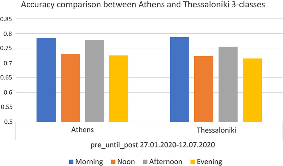

Especially, in the case of 3-classes experiments our model performed identically between the two cities as Fig. 16 showcases. Specifically, in each time interval accuracy was almost equal between the two cities, indicating our model’s stability. Although traffic levels are higher in Athens, our proposed model is reliable in both cities. Therefore, our modelling framework is validated in both cities.

5. Evaluation and discussion

This section discusses our findings and compares these with earlier findings [1]. While our early work focused on extracting conclusions regarding individual sensors, current work examines the whole set of sensors, and compares results for the two cities. An early conclusion from the initial effort [1], was that data subsets including abnormal/atypical traffic periods (mostly holidays) performed better than the corresponding trimester with the lowest abnormalities (15.09.2019–20.12.2019).

Based on that, it was decided to exploit the heavily disruptive period of the COVID-19 related imposed lockdown. The initial model contained only weather metrics and was not discriminating between weekdays and weekends. The dataset range was approximately six months, from August 2019 to January 2020. The current work includes a binary variable that distinguishes weekends, as well as a new feature regarding the lockdown, while expanding the range until August 2020. The following subsections briefly compare conclusions from our earlier work and new findings.

5.1 Discussion on early results

Both efforts utilize the same two classifiers: Random Forest and Logistic Regression. The difference in performance among the two classifiers was deemed insignificant with minor deviations. The same conclusion emerges from the current findings. On top of that, Random Forest needs approximately 10 times longer hyper-parameters tuning. Thus, the selection can be based on individual needs in terms of training and adaptation speed vs. accuracy. Respectively, related works suggest either Random Forest [7] or Decision Trees [6] as top performers.

Another important part was that in the 3-classes case, the accuracy of the previous model barely exceeded that of a baseline model. However, processing more data and the addition of a new variable that distinguishes weekdays from weekends resulted in an impressive (23%) accuracy leap. The same conclusion applies for both cases (2 and 3-classes). In fact, for Morning the accuracy (82%) for 3 classes was very close to that of Evening in 2 classes (82%). In both works, time intervals other than Morning and Afternoon resulted in a considerable drop in accuracy.

As further verification of earlier findings, new results confirm that adding more data does not always result in higher accuracy. Similarly to our earlier work, the best scores were not achieved by training the whole dataset.

5.2 Evaluation 3–4 months

Selecting multiple splits to the dataset reveals points worth discussing, after observing the results emerging from a 10-fold cross-validation. The first point is that quadrimester splits produce better results for most of the cases. The line indicating the whole dataset (13 months) is common in Figs 9 and 10, however it does not achieve better results than the corresponding subset of the lockdown and post-lockdown period at any interval during the day.

An interesting observation is that the newly introduced day interval named Noon always produces worse results than the corresponding Afternoon one, while it only once scores higher than Morning. Afternoon produces the best results (88%) for the case of two classes in both splits (3 and 4 months) and seems to be the most predictable interval among those examined. The Evening interval has the lowest traffic load and for both splits it fails to withstand.

When the dataset is split into 3 classes the results during the day differ (see Appendix A). The Morning interval gives better results than the rest, but still Afternoon outperforms Noon. Even though Morning and Evening intervals have the lowest loads of traffic throughout the dataset range, they do not share similar predictability. Evening usually underperforms all others, however in the case of the 4-month split it achieves accuracy similar ( $\sim$ 1%) to Noon.

5.3 Weekday vs. weekend

A period of undoubted traffic variation is weekends. The literature is unclear whether weekdays should be processed without weekends or models should consider them as a whole [15, 16].

Besides the fact that previous work segregated data as such, weekends as a binary feature was the dominating factor for this work. In general, this tagging was expected to show increased accuracy in advance, because those instances (weekends) present significantly less traffic congestion. Thus, the target variable on those instances is expected to be lower than the median value (class Low), bearing in mind that weekends are fewer than weekdays.

However, based on recursive feature elimination, it is impressive that it achieves approximately three times higher importance than any weather condition metric. The evaluation of this addition is positive, and it is considered of high significance for future research, as it is not an expensive and hard to capture feature like the rest utilized by the model.

5.4 Morning/noon/afternoon/evening

Time intervals of interest during a day can vary. In small cities normally the focus is mostly until afternoon. In this case both cities are quite large (Athens with over 4 million population, and Thessaloniki with over 1 million) and considered busy until very late. Thus, multiple splits were examined. In addition to our earlier work, a new subset of the same duration (3 hours), named Noon was introduced and captured data from 12:00 to 15:00. It is identified as peak hours but differs from other findings [37].

Prior observations [1] had shown that the load of traffic congestion was lower for Morning, while the new data which contain information for a whole year reflect a slightly different conclusion. Indeed, the current dataset reveals that the lowest traffic load is linked with Evening, followed by Morning. By having a bigger dataset, Noon and Afternoon are still the most heavily loaded intervals during the day.

Another significant observation is that for the Evening interval the new model struggles to compete with the rest, while for the original model, without the addition of the new features, it was the only prominent one. Overall, Morning and Afternoon intervals outperform the rest, even for the cases of the whole model and the lockdown segmentation.

5.5 COVID-19/lockdown

Unfortunately, 2020 contained a concurrent lockdown for both cities which -inevitably- heavily affected traffic. Indicatively, the levels of traffic were even lower than these in the middle of August which traditionally is considered in Greece to be the peak of vacations, thus traffic congestion is extremely low in both cities.

For this approach we decided to form a time range of interest based on the length of the lockdown period (56 days). In other words, we chose one subset of 56 days for the pre-lockdown period and another for the post-lockdown with the goal to compare the model for all three periods.

Based on that, the periods during and after lockdown scored approximately 10% worse than the pre-lockdown period. During the lockdown period the algorithm regarding Afternoon had the worst accuracy among all experiments, while Noon was marginally the best. Interestingly, combining all three subsets (“pre_until_post” period) the best accuracy (88%) achieved, was even higher than the score for the whole dataset (86%), as seen in Figs 11 and 12. Consequently, more data records do not necessarily lead to a better performance.

Finally, a validation of the trends is that the new model trained on the whole dataset has very similar (in terms of deviation) results to the whole COVID-19 related split of data from 27 January to 12 July. Similarly to the previous subsection, the same experiments were performed for all time intervals during the day for the 3-class split (see Appendix C). For the case of 3-classes, again, the Morning interval scores higher accuracy while the whole model also has very similar results to the merged lockdown-split.

5.6 Athens vs. Thessaloniki

Undoubtedly, Athens is more populated than Thessaloniki and attracts more tourists throughout the year. Considering that traffic is positively correlated to the population, higher jam factor values for Athens are explainable. However, the similarities between the two cities in daily activities lead to analogous patterns before and after COVID-19 restrictions. The results indicate that the model performs better with data from Athens in the Morning and at Noon, while similar performance is observed in the rest intervals. However, in the case of 3-classes, accuracy levels throughout the day are almost identical between the two cities, having the model trained on the proposed “pre_until_post” subset.

5.7 Threats to validity

Many scientific efforts analyze and examine their questions based on several assumptions. Most of the time those assumptions are raised due to unknown factors, limited data, or personal estimations. The validity of results and conclusions with assumptions is highly connected.

A crucial assumption of this work relies on the fact that the model developed needs accurate predictions of day-ahead weather conditions, which is not always feasible. Another threat is that 2020, due to the pandemic, seems to affect the post-lockdown load of traffic and thus the results may differ from previous years. In addition, transforming the problem into balanced classification may slightly affect the accuracy of the model since abnormal instances may not affect the split point the same way the mean value might do.

6. Conclusions and future work

The purpose of this paper was to examine how different intervals during the day and year can affect day-ahead traffic forecasting, while also assessing the effect of long atypical conditions (in our case-lockdown) in the predictability. The main aspects of the proposed model are weather metrics, combined with features describing weekends and the lockdown. In general, the fragmentation of the dataset was extensive. The dataset was initially split into four intervals during a day (Morning, Noon, Afternoon, Evening) and consecutive trimesters and quadrimesters along the whole range. On top of that, findings led to the decision for a further split adjusted for the lockdown period which lasted 56 days in Greece.

6.1 Conclusions

The major factor that boosted the model’s performance was the distinction of weekends. Besides that, having a new variable that marks the status of days, regarding lockdown presence, also rewarded the model with a small increase.

In between, transforming the target variable into three classes resulted in remarkably lower accuracy (besides the Morning subset), however it justified some findings regarding day intervals.

A clear conclusion is that the model was more successful for Morning and Afternoon. This is probably because these splits coincide with the beginning and the end of work for most of the working population. Also, the Evening interval does not stand out in comparison with the rest. This can be speculated to be because weather metrics, such as UV and humidity, do not add much variation. The Evening interval though has the lowest load of traffic, thus its predictability may be affected in a negative way.

The splits regarding Spring achieved higher accuracy, but this rather happened because of the explosion of the pandemic. The constructed subset based on the lockdown era, consisting of 168 days, clarified that dataset with equally mixed data scored consistently higher, and Morning and Afternoon intervals were again the most reliable. Consequently, in case of special events, it is suggested that training of models should be equal for each period.

Overall, our aim was to develop a model capable of predicting traffic levels, while special events (lockdown) exist, or during transitional periods (after a lockdown). However, our model can be applied under normal conditions as well. Figure 11 presents the “pre-lockdown” period (normal conditions) with 84% accuracy, without training on the desired subset. In addition, even during normal conditions, there are events that affect traffic (road maintenance, sports/social events, strikes). Thus, these events could temporarily have effects similar to a lockdown. Our methodology is robust to special events and our proposed model works.

The comparison between Athens and Thessaloniki indicates that our model is adjusted in both cities, having the model trained on the “pre_until_post” subset. As there is no significant differentiation in performance both in 2-classes and 3-classes experiments, our model could be considered stable.

It seems that higher traffic load does not guarantee higher accuracy, since even though the Noon split had higher traffic load, it did not outperform the rest at any point. On the other hand, the Evening interval which marked the lowest traffic load, performed worse for almost every scenario.

Also, testing the model on the whole dataset did not result in better performance, thus it is concluded that a bigger training set does not directly improve accuracy. This means that similar models in order to remain competitive in terms of accuracy should be deployed with a clear target period and not arbitrarily be trained on all available data.

Weather conditions are also considered as metrics subject to high correlations, however the correlation is not stable throughout a year period, thus it could affect each training subset individually. To summarize, traffic prediction is a problem with extended seasonality and training data should be carefully chosen to preserve relations amongst different periods.

Based on that, the proposed methodology can be used both as a standalone model that predicts day-ahead traffic (for travel planning) and as an assistance feature in a more sophisticated and complex system, since it can provide significant insights into the peculiarity of training data. Our purpose is to assist professionals that build traffic prediction systems, to understand the significance of weather data even for long-term scenarios, while endorsing the unique characteristics that each day interval and time slot is accompanied with. Lastly, the scientific merit is the validation of prior results [1] regarding the fluctuation of accuracy on each training subset and especially the positive effect of utilizing data for periods depicting movement restrictions such as the ongoing pandemic of COVID-19.

Our contribution includes a novel methodology for predicting day ahead (long-term) traffic state based on weather data as well as status information regarding weekends and lockdown. The methodology incorporates data engineering and preprocessing as well as model construction. Our findings suggest that our model, trained on the proposed subset “pre_until_post”, performs better (88%) than on the whole dataset (86%). Our prior work [1] is validated and extended by the new findings. Key new contributions include the exploration of the impact of weekends and/or lockdown limitations, a new timeslot for the noon rush hour. Another point that this work underlines is that such a model could also be replicated in different cities, since both Athens and Thessaloniki had similar effects and results. In addition, prior literature findings such as the huge difference in impact between weekdays and weekends [12, 29, 36]were also justified.

6.2 Future work

This work provides interesting insights into traffic prediction, some rather unexpected. There may be limited scope to further investigate the day interval splits. However, the splits throughout the year may reveal significant points in order to adopt the model and the potential is considered substantial. Feature-wise it would be interesting to also focus on the weather icon (snow, rain etc.) or holidays and examine current conclusions. Lastly, possible future movement restrictions could assist in further validating existing conclusions. The consecutive lockdowns are expected to have different magnitudes and compliance by the citizens.

Lastly, that kind of effort could also be applied by utilizing different kinds of data. Traffic load can also be expressed through OD demand estimation which offers a much broader coverage over the area of interest [42], and thus can eliminate any hesitation about balance while comparing a model amongst data gathered from different cities.

Footnotes

Acknowledgments

We would like to thank DOTSOFT S.A. for providing the sensor data required for our experiments.

Appendix A

Figure A1.

Results on 3-month and 4-month periods for 3-class experiments.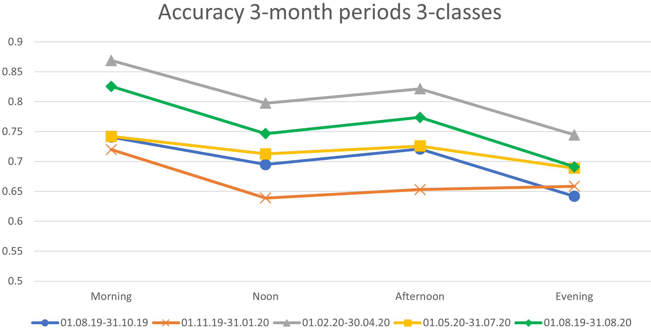

Appendix B

Figure B1.

Jam Factor throughout lockdown periods.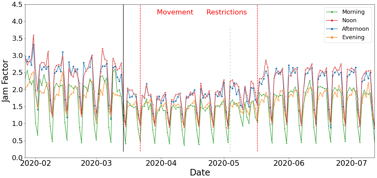

Appendix C

Figure C1.

Results before, during and after lockdown periods for 3-class experiments.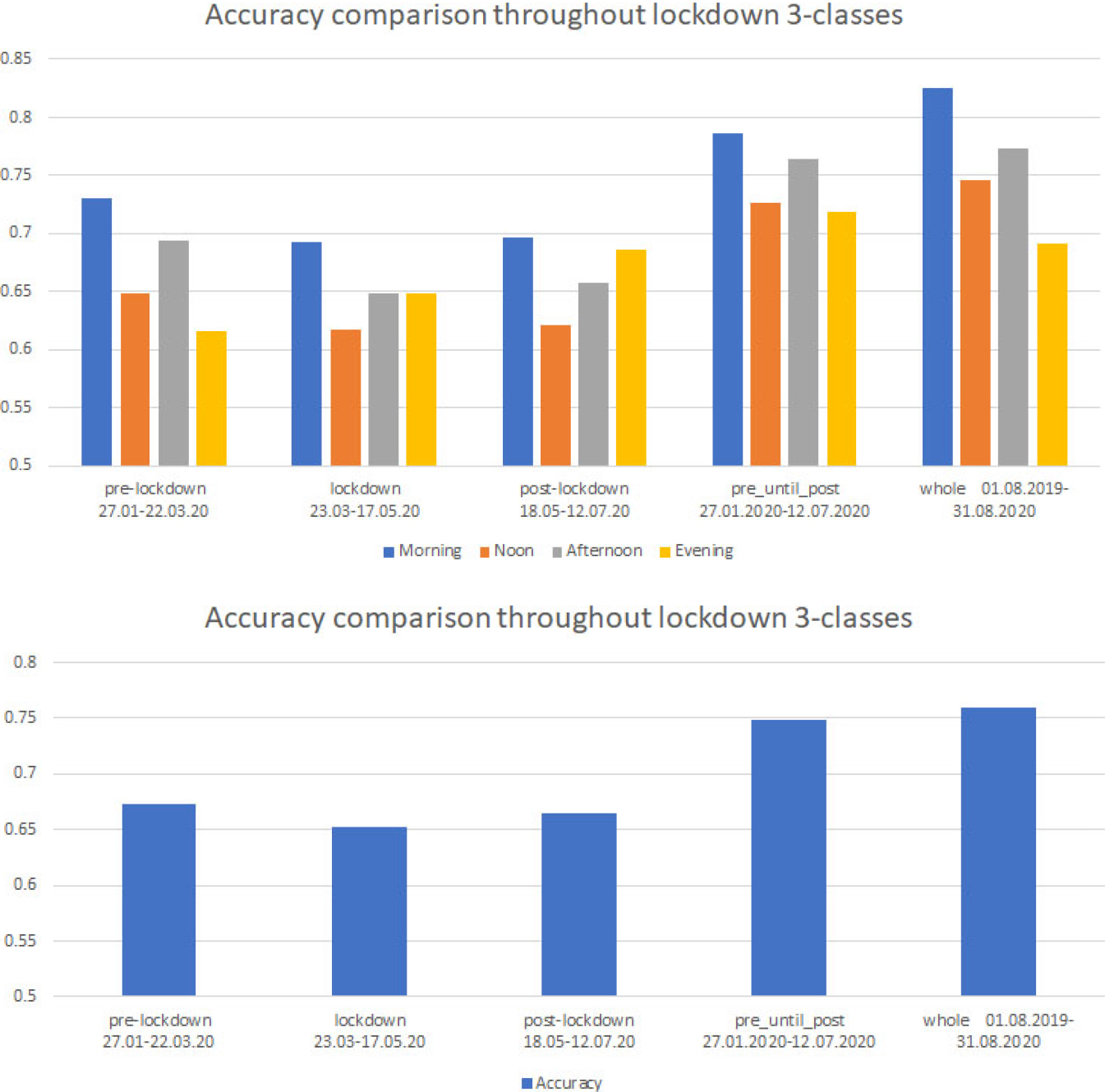

Table D1

Accuracy comparison between Athens and Thessaloniki for 2-class experiments for the whole dataset

Time Interval	Athens	Thessaloniki
Morning	89.52%	86.39%
Noon	87.26%	84.21%
Afternoon	89.36%	87.41%
Evening	82.79%	81.89%
Average	87.23%	84.98%

Appendix D

References

Christantonis

Tjortjis

Manos

Filippidou

Mougiakou

Christelis

. Using classification for traffic prediction in smart cities. IFIP Int’l Conf on Artificial Intelligence Applications and Innovations. Springer, Cham. 2020; p. 52-61.

Vlahogianni

Karlaftis

Golias

. Short-term traffic forecasting: Where we are and where we’re going. Transportation Research Part C: Emerging Technologies. 2014; 43: 3-19.

Nejad

Seifi

Ahmadi

Seifi

. Applying data mining in prediction and classification of urban traffic. WRI World Congress on Computer Science and Information Engineering. IEEE. 2009; p. 674-678.

Wang

Chen

Qin

Zhu

. Dynamic traffic prediction based on traffic flow mining. 2006 6th World Congress on Intelligent Control and Automation IEEE; 2006. p. 6078-6081.

Yan

. Short-term traffic condition prediction of urban road network based on improved SVM. 2017 Int’l Smart Cities Conf. (ISC2) IEEE. 2017; p. 1-2.

Mystakidis

Tjortjis

. Big data mining for smart cities: Predicting traffic congestion using classification. 11th IEEE Int’l Conf on Information, Intelligence, Systems and Applications, 2020.

Hashemi

Almasi

Ebrazi

Jahanshahi

. Predicting the next state of traffic by data mining classification techniques. Int’l Journal of Smart Electrical Engineering. 2012; 1(3): 181-193.

Liu

Choudhary

Zhou

Khokhar

. A scalable distributed stream mining system for highway traffic data. European Conf on Principles of Data Mining and Knowledge Discovery, PKDD 2006: Knowledge Discovery in Databases: PKDD 2006. Springer, Berlin, Heidelberg; 2006. p. 309-321.

Pan

Demiryurek

Shahabi

. Utilizing real-world transportation data for accurate traffic prediction. 2012 IEEE 12th Int’l Conf on Data Mining. IEEE; 2012. p. 595-604.

10.

Theodorou

Salamanis

Kehagias

Tzovaras

Tjortjis

. Short-term traffic prediction under both typical and atypical traffic conditions using a pattern transition model. 3rd Int’l Conf on Vehicle Technology and Intelligent Transport Systems. SciTePress; 2017. p. 79-89.

11.

Bai

Zhong

Sun

Zhao

. Traffic flow prediction based on expressway operating vehicle data. 2018 11th Int’l Conf on Intelligent Computation Technology and Automation (ICICTA). IEEE; 2018. p. 322-326.

12.

Clark

. Traffic prediction using multivariate nonparametric regression. Journal of Transportation Engineering. 2003; 129(2): 161-168.

13.

Qiao

Haghani

Hamedi

. Short-term travel time prediction considering the effects of weather. Transportation Research Record: Journal of the Transportation Research Board. 2012; 2308(1): 61-72.

14.

Zhang

Cheng

Ren

. A graph deep learning method for short-term traffic forecasting on large road networks. Computer-Aided Civil and Infrastructure Engineering. 2019; 34(10): 877-896.

15.

Zhang

Kabuka

. Combining weather condition data to predict traffic flow: A GRU-based deep learning approach. IET Intelligent Transport Systems. 2018; 12(7): 578-585.

16.

Liu

. Prediction of road traffic congestion based on random forest. 2017 10th Int’l Symposium on Computational Intelligence and Design (ISCID). IEEE; 2017. p. 361-364.

17.

Medrano

Aznarte

. A spatio-temporal attention-based spot-forecasting framework for urban traffic prediction. Applied Soft Computing. 2020; 96: 106615.

18.

Hou

Gao

Kang

Chen

, and Patz

. Intra-county modeling of COVID-19 infection with human mobility: Assessing spatial heterogeneity with business traffic, age and race. (2020) medRxiv.

19.

Aletta

Brinchi

Carrese

Gemma

Guattari

Mannini

, et al. Analysing urban traffic volumes and mapping noise emissions in Rome (Italy) in the context of containment measures for the COVID-19 disease. Noise Mapping. 2020; 7(1): 114-122.

20.

Dong

Gardner

. An interactive web-based dashboard to track COVID-19 in real time. The Lancet Infectious Diseases. 2020; 20(5): 533-534.

21.

Adeli

Ghosh-Dastidar

. Mesoscopic-wavelet freeway work zone flow and congestion feature extraction model. Journal of Transportation Engineering. 2004; 130(1): 94-103.

22.

Jiang

Adeli

. Wavelet packet-autocorrelation function method for traffic flow pattern analysis. Computer-Aided Civil and Infrastructure Engineering. 2004; 19(5): 324-337.

23.

Jiang

Adeli

. Dynamic wavelet neural network model for traffic flow forecasting. Journal of Transportation Engineering. 2005; 131(10): 771-779.

24.

Ghosh-Dastidar

Adeli

. Neural network-wavelet microsimulation model for delay and queue length estimation at freeway work zones. Journal of Transportation Engineering. 2006; 132(4): 331-341.

25.

Dunne

Ghosh

. Weather adaptive traffic prediction using neurowavelet models. IEEE Transactions on Intelligent Transportation Systems. 2013; 14(1): 370-379.

26.

Kong

Liu

. Short-term traffic volume prediction using classification and regression trees. 2013 IEEE Intelligent Vehicles Symposium (IV). IEEE; 2013. p. 493-498.

27.

Abdel-Aty

Pemmanaboina

. Calibrating a real-time traffic crash-prediction model using archived weather and ITS traffic data. IEEE Transactions on Intelligent Transportation Systems. 2006; 7(2): 167-174.

28.

Tang

Liu

. Short-term traffic flow prediction considering spatio-temporal correlation: A hybrid model combing type-2 fuzzy c-means and artificial neural network. IEEE Access. 2019; 7: 101009-101018.

29.

Christantonis

Tjortjis

. Data mining for smart cities: Predicting electricity consumption by classification. 2019 10th Int’l Conf on Information, Intelligence, Systems and Applications (IISA). IEEE; 2019. p. 1-7.

30.

Ganji

Shekarrizfard

Harpalani

Coleman

Hatzopoulou

. Methodology for spatio-temporal predictions of traffic counts across an urban road network and generation of an on-road greenhouse gas emission inventory. Computer-Aided Civil and Infrastructure Engineering. 2019; 35(10): 1063-1084.

31.

Zhang

Zhou

Chen

Zhang

. Network-wide traffic speed forecasting: 3D convolutional neural network with ensemble empirical mode decomposition. Computer-Aided Civil and Infrastructure Engineering. 2020; 35(10): 1132-1147.

32.

Liu

Lyu

. A spatio-temporal ensemble method for large-scale traffic state prediction. Computer-Aided Civil and Infrastructure Engineering. 2019; 35(1): 26-44.

33.

Ferreira

Poco

Freire

Silva

. Visual exploration of big spatio-temporal urban data: A study of new york city taxi trips. IEEE Transactions on Visualization and Computer Graphics. 2013; 19(12): 2149-2158.

34.

Antoniou

Koutsopoulos

Yannis

. Dynamic data-driven local traffic state estimation and prediction. Transportation Research Part C: Emerging Technologies. 2013; 34: 89-107.

35.

Wen

Zhang

Sun

Wang

. A hybrid temporal association rules mining method for traffic congestion prediction. Computers & Industrial Engineering. 2019; 130: 779-787.

36.

Gecchele

Rossi

Gastaldi

Caprini

. Data mining methods for traffic monitoring data analysis: A case study. Procedia - Social and Behavioral Sciences 2011; 20: 455-464.

37.

Necula

. Analyzing traffic patterns on street segments based on GPS data using R. Transportation Research Procedia. 2015; 10: 276-285.

38.

Guide - HERE SDK for Android (Navigate Edition) - HERE Developer [Internet]. HERE Developer. 2021 [cited 12 June 2021]. Available from: https://developer.here.com/documen-tation/android-sdk-navigate/4.6.2.0/dev_guide/topics/routing.html#find-traffic-along-a-route

39.

Ayman

Wilbur

Sivagnanam

Pugliese

Dubey

Laszka

. Data-driven prediction of route-level energy use for mixed-vehicle transit fleets. 2020 IEEE Int’l Conf on Smart Computing (SMARTCOMP). IEEE; 2020. p. 41-48.

40.

Zhu

Mehrabi

Xiao

Wen

. CrowdParking: Crowdsourcing based parking navigation in autonomous driving era. 2019 Int’l Conf on Electromagnetics in Advanced Applications (ICEAA). IEEE; 2019. p. 1401-1405.

41.

Basak

Dubey

Bruno

. Analyzing the cascading effect of traffic congestion using LSTM Networks. 2019 IEEE Int’l Conf on Big Data (Big Data). IEEE; 2019. p. 2144-2153.

42.

Caceres

Wideberg

Benitez

. Review of traffic data estimations extracted from cellular networks. IET Intelligent Transport Systems. 2008; 2(3): 179.