Image binarization method for markers tracking in extreme light conditions

Abstract

Image binarization is one of the fundamental methods in image processing and it is mainly used as a preprocessing for other methods in image processing. We present an image binarization method with the primary purpose to find markers such as those used in mobile 3D scanning systems. Handling a mobile 3D scanning system often includes bad conditions such as light reflection and non-uniform illumination. As the basic part of the scanning process, the proposed binarization method successfully overcomes the above problems and does it successfully. Due to the trend of increasing image size and real-time image processing we were able to achieve the required small algorithmic complexity. The paper outlines a comparison with several other methods with a focus on objects with markers including the calibration system plane of the 3D scanning system. Although it is obvious that no binarization algorithm is best for all types of images, we also give the results of the proposed method applied to historical documents.

Keywords

Real-time markers tracking light reflection non-uniform illumination

1. Introduction

1.1 Motivation

The technology of 3D scanning has become indispensable in many fields of science and industry. Structured light scanning systems use markers for coupling more scans into one and in the calibration process. Finding markers in both cases must be a robust operation. But, under extreme conditions such as light reflection or non-uniform illumination, it can be a very demanding task. It is understood that wrong marker positions cause incorrect calibration parameters, i.e., incorrect mathematical models, which causes distorted and incorrectly scaled scans of the desired object. However, inaccurately determined marker positions on an object cause incorrect geometry coupling, and in the case of several scans, the included coupling error may be unacceptable.

1.2 Background and applications

Marker tracking is based on determining corners (variations of the Harris algorithm), boundaries of shapes (variations of the Canny algorithm), components of binarization image, etc. When it comes to high light reflection, algorithms for marker tracking have a problem with robustness. For example, various versions of the Harris algorithm may detect too many corners and, using all of them, determining markers (square shapes) is quite complicated. Furthermore, the Canny algorithm may produce too many interrupted lines that do not bound any marker. If we try to set the parameters of both above algorithms in a way to avoid too many corners or too many interrupted lines, there is a high possibility some important markers will be undiscovered. In general, many algorithms use some heuristic parameters where a precise setup is required. Otherwise, it is almost like iterative algorithms that have neither linear nor (especially not) constant algorithmic complexity. The main goal is finding a balance between time-consuming costs and quality in using image binarization in real-time applications. In addition to markers (objects) tracking, image binarization finds numerous applications in historical document analysis and recognition [27], creating super-resolution medical 3D images [37], human facial expressions [1, 10], visual odometry for moving urban environments [7], people tracking [6, 11], textile industry [5], optimization [28, 34, 43], pattern recognition problems [12, 20], robotics [24, 40, 42], etc.

The rest of this paper is structured as follows.

Section 2 outlines related work. Section 3 describes the proposed method. Section 4 reports the results, including comparisons with some other methods. Section 5 brings the discussion, and Section 6 concludes this paper. Finally, Section 7 announces the future work.

2. Related work

As it is presented in the review work of Ismail et al. [13], image binarization can roughly be divided into two main categories: global and local, where their combination presents a hybrid method.

Image binarization as input uses a grayscale image with a value range within 0–255 and outputs an image where the value 0 corresponds to a black pixel and where the value 255 corresponds to a white pixel.

In the global case, for an input grayscale image $I$ , output image $B$ , and for threshold $T$ , the grayscale image becomes binary in the following way: $B(x,y)=$ 255 for $I(x,y)\geqslant T$ , $B(x,y)=$ 0 for $I(x,y)<T$ , where $I(x,y)$ presents intensity value of a pixel in location ( $x, y$ ). The threshold calculation is mainly based on the histogram, clustering, entropy, and particular objects. The term sub-image used in this paper refers to the square neighborhood of a pixel position ( $i, j$ ) where that position is the center of the neighborhood.

On the other hand, in the case of a local type of binarization, the threshold value is calculated for each pixel based on the local characteristics of its neighborhood (mean value, standard deviation, minimum and maximum value, statics moment, etc.), where the calculation is often accompanied by heuristic parameters.

In the same paper [13], the authors compared the most relevant methods from this area. They have briefly described algorithms and their advantages and drawbacks in conditions such as non-uniform illumination.

In the case of strong light reflection, and in the case of non-uniform illumination, images contain stains that resemble blurred pepper noise, and the local intensity varies a lot. Hence, global methods such as (Otsu [22]; Liu and Sri-Hari [44]) are inferior in comparison with methods based on local characteristics since the threshold value $T$ depends on intensity distribution.

Calculating the threshold value for each pixel based on the mean value and the standard deviation of its neighborhood and adaptive calculation of the threshold value based on the mean value of sub-image (Niblack [21], Sauvola and Pietikainen [31]) are the two basic ideas from which numerous variations have been made.

Lins et al. [17] outlined the binarization approach suitable for complex documents. The scheme automatically decomposes a document image and identifies each of the graphical elements to provide a suitable binarization for each of them independently. At the end of the binarization phase of all the elements, the image is re-assembled to obtain the binary high-quality version of the original document. Execution time is too long to use in the proposed application.

Singh et al. [33] presented a new adaptive binarization method for the degraded document images where four steps are applied: contrast analysis, contrast stretching, thresholding by the global threshold, and noise removal. The method is conceptually quite like the proposed method. The methods differ in the function that returns the local threshold value as well as in the parameters used within the function. Based on a relative comparison of time consumption, the algorithm is slightly slower than the other algorithms we compared with the proposed method (Table 1).

In [18] the authors address the document image binarization problem with a three-part procedure: removing background information from the image, separation of the remaining misclassified background and character pixels using a local co-occurrence mapping and local contrast. For the same reason as previous work, we also exclude this method.

Kesiman et al. [14] implemented the construction of ground truth binarized images. For the image binarization, inter alia, the authors applied contour detection by the Prewitt operator, Otsu’s global thresholding method, noise reduction by Median filter, and constrained local-global Otsu’s method. The algorithmic combination of this approach may also be applied to our case but setting the parameters for individual algorithms requires significant effort.

Several other papers are relevant for this purpose of use and give useful results (Wen et al. [41], Vo et al. [39]), but the execution time is too large which excludes them from further consideration and we do not make comparisons with them.

In [36] the authors presented an image binarization method based on a fully convolutional neural network. Convolutional neural networks are also contained in [38], where the authors use the image binarization method to detect musical notation. Both papers are based on neural networks and are therefore excluded due to their algorithmic complexity.

We also take note of two review papers. In the first of them [26], the authors present a competition on document image binarization in conjunction with the ICDAR 2017 conference. This paper includes the evaluation measures used and the performance of the 26 submitted methods along with a brief description of each method.

In the second one Mustafa et al. [19], outline review of different binarization approaches on degraded document images is presented, where several binarization techniques such as Bernsen [2, 8], Multiple Thresholding [23], and Deghost method [19] have been selected for comparison and applied on the H-DIBCO dataset.

In what follows, the proposed method is compared with one method which belongs to the global type of binarization Otsu [22] and with several local type binarization methods: Shi et al. [32], Saha and Ray [29], Niblack [21], Kittler and Illingworth [16], Bradley, Roth [4], Bernsen [2] and Feng and Tan [9].

The Otsu method assumes the division of pixels in two classes and calculates the threshold that divides the classes in a way that minimizes the covariance between them. The Niblack [21] method calculates the threshold value based on the mean value and standard deviation of the sub-image.

Saha and Ray [29] outlined an iterative method that belongs to the local type of binarization. For input image $I$ and current output image $C$ (initially $C=I$ ) which changes in each iteration, the method minimizes the energy function, where it presents the difference of the image $I$ and current image $C$ , over the edge, presents the norm of the gradient and defines the edge. The calculation is time-consuming and the method is too locally-oriented what leads to too many small regions inside markers (Fig. 5). Figure 5 shows that non-uniform illumination does not affect the result.

The method (Shi et al. [32]) is also an iterative method that belongs to the local type of binarization where the image is separated into square regions, and for each of the regions, the threshold value is calculated. The flat parts within the histogram of each area represent peaks, while the curved parts (valleys) within the histogram represent the threshold value. By using the Bhattacharya coefficient [3], the similarity between the histograms is measured and the best candidate represents the global threshold value.

Feng and Tan [9] present a local thresholding method based on the local mean, the minimum, and the standard deviation of two adaptively calculated local windows.

In the paper titled “Comparison of Niblack inspired binarization methods for ancient documents” [15] the authors present a local thresholding technique and give a detailed comparison of Niblack inspired binarization methods. In addition to the Niblack factor, the authors use the mean grey value and the number of pixels in calculating the local threshold.

Bradley and Roth [4] outlined a local thresholding method very similar to the proposed method where the authors set each pixel of the image to black value if its intensity is a certain percent lower than the average brightness of the sub-image pixels, otherwise, it is set to white. The proposed method can be considered as an adaptive upgrade of the Bradley and Roth methods.

3. Proposed method

The proposed method belongs to the hybrid type of binarizations. The size of the sub-image is estimated adaptively, but the binarization method with a fixed sub-image size Eq. (1) is used for this estimation.

Manually setting the sub-image size, as in Eq. (1), generally provides satisfactory quality results, and further improvement of the sub-image size is not necessary in most cases.

Yet, adaptive calculation of the sub-image size in some cases provides additional improvements and gives robustness.

Based on several local parameters: global median intensity, mean and median sub-image value, and pixel intensity value, the proposed method calculates whether the pixel belongs to the object or the background.

Figure 1.

Flow chart of the proposed algorithm.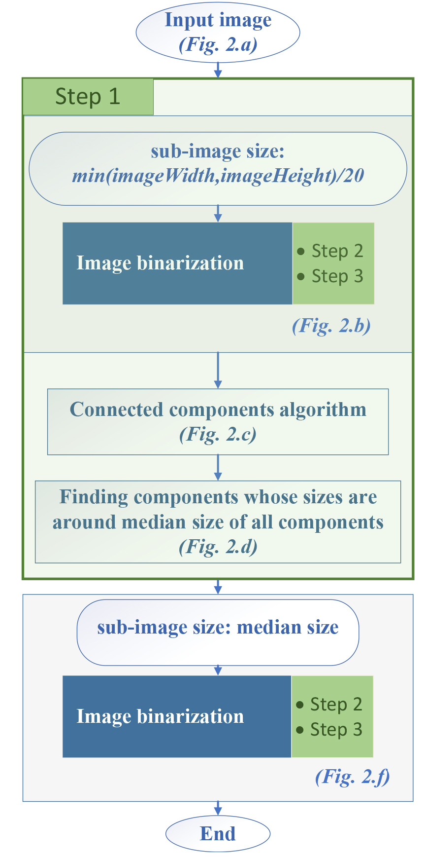

Figure 2.

Proposed adaptive calculation of sub-image size. a) Input image; b) proposed binarization with sub-image size set by (1); c) result of a connected component algorithm; d) components whose sizes are around the median size of all components; e) the way of calculating component size with width and height; f) proposed binarization with sub-image size as the size of the median component.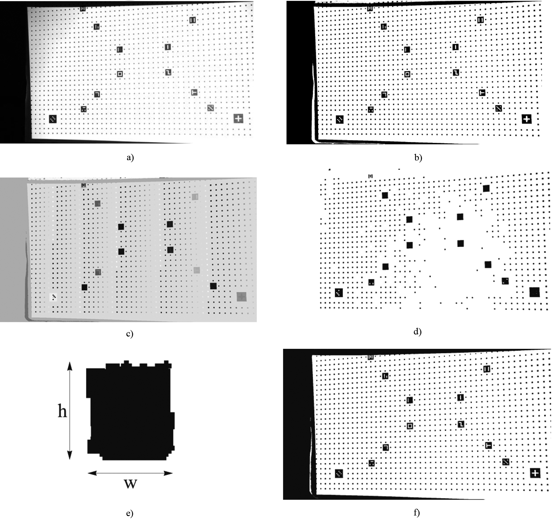

The steps of the proposed algorithm are graphically presented in the flow chart (Fig. 1), and here we describe them textually:

Adaptive calculation of sub-image size (Fig. 1, Step 1).

Calculating average and median pixel intensity inside given sub-image for each pixel. The key of this step is algorithm complexity $O$ (1) (Fig. 1, Step 2).

Based on the global median intensity of the whole image, average and median intensity of the sub-image, and the pixel intensity itself, it is calculated whether the pixels belong to the object or background (Fig. 1, Step 3).

3.1 Estimation of sub-image size

If the binarization involves an image that contains regions such as markers (Fig. 2), the approach to estimating the sub-image size is completely autonomous and adaptive (Figs 1 and 2).

We set sub-image size to the fixed value:

(1)min(imageWidth, imageHeight)/20.

Using this value, the method goes through the remaining two steps of the proposed algorithm (2 and 3). In this way we get a binarization image for the initial fixed sub-image size (Fig. 2b).

The idea is to find the average size of connected components within that image and estimate the global sub-image size based on that value. Hence, we apply the Connected component algorithm [30] onto the binarization image from the previous step (Fig. 2b) and obtain the image containing the connected components as a list of the positions of the connected pixels with the same intensity (Fig. 2c). For each component, we calculate the area of its minimum rectangular frame (Fig. 2e). Then, those components in which the area is several times larger or smaller than the median area are going to be removed from the image (Fig. 2d).

In this way, the components that represent noise are eliminated as well as the component that represents the background. The mean value of the height and width of the remaining components is set for the core size. After the sub-image size is calculated, step 2 is the next station of the approach.

In the cases where the image contains a lot of noise and there are nondominant homogeneous regions, instead of this adaptive step, we can just manually set the size of the sub-image to (1) and then go to step 2.

The algorithmic complexity of the connected components algorithm depends on the noise level of the input binary image. Since the results of our method are not noisy, algorithmic complexity tends to be constant complexity.
3.2 Mean and median value of the sub-image with algorithm complexity O(1)

The next step of the proposed algorithm, within algorithm complexity $O(1)$ , is to find the mean and median value of the sub-image to be used in last step 3. Of course, finding the mean and median values of sub-image for each pixel is a simple task if we ignore the time of calculation. The key to this step lies in the constant algorithm complexity. The whole idea can be found in [25] where the authors outline the Median filter with $O$ (1) complexity. Also, in [33] the authors used a similar approach. Here we present a summary of that idea as well as its application to our problem. The pixel intensity of a grayscale image is within the range of 0 to 255. To calculate the mean and median sub-image value of each pixel, the histogram $H$ as a field of 256 elements for each possible intensity of 0 to 255 is used where all elements of the histogram are initialized to 0. In what follows, $r$ presents the sub-image size calculated in the previous step, under $p_{i,j}$ we refer to the pixel intensity of its position ( $i, j$ ) in the image $I_{\textit{mage}}$ . The full sub-image histogram of the pixel ( $i, j$ ) is signed as $H_{i,j}$ , and the sub-image column histogram is denoted as $H_{j}$ . The location ( $i, j$ ) is the center of its sub-image histogram. By adding an intensity $p$ into the histogram $H_{i,j}$ , the value $H_{i,j}[p]$ increments by 1. Likewise, by removing an intensity $p$ from the histogram $H_{i,j}$ , the value $H_{i,j}[p]$ decrements by 1. The same applies to column histograms $H_{j}$ . Based on this, for two sub-images A and B, and any histogram H, $H\left({A\cup B}\right)=H\left(A\right)+H\left(B\right)$ is valid. All this is additionally described in Fig. 3.

Figure 3.

The manipulation with histograms. a) The vertical change of the column histograms; b) The sum of r column histograms – removing first column histogram from the left side and adding new column histogram from the right side.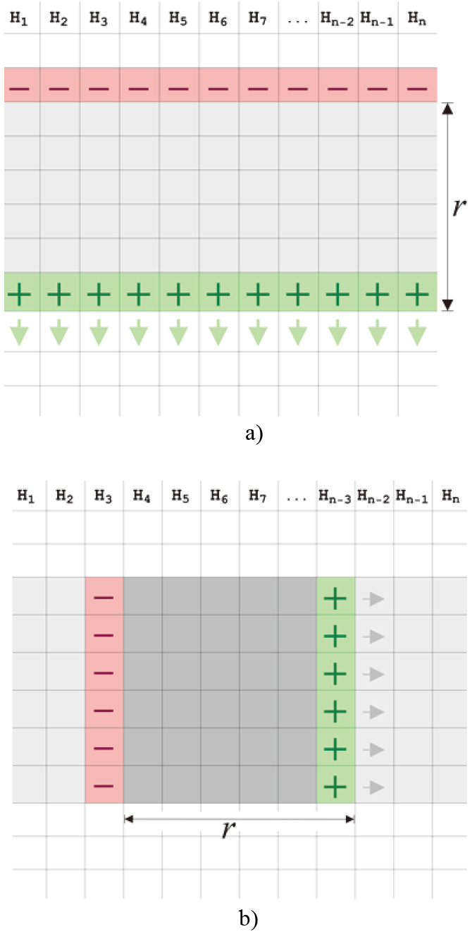

By increasing the pixel index $j$ we remove the first column histogram $H_{j-r}$ from the left side and add a new column histogram $H_{j+r}$ to the right side. After that, we have the new $H_{i,j}$ .

Figure 4.

Mean intensity value of the sub-image in the calculation of sensitivity to reflection.

To calculate the mean and median sub-image value for each pixel ( $i, j$ ) inside $I_{\textit{mage}}$ , the histogram $H_{i,j}$ as the union of column histograms $H_{j,\ldots,j+r}$ needs to be calculated.

The median value of the histogram $H_{i,j}$ is the position in histogram from 0 to 255 where the sum of histogram elements starting from the beginning becomes equal to or greater than the half number of histogram elements ( $r^{2}$ /2). Similarly, we calculate the mean value.

Figure 5.

The comparison of image binarization algorithms for the 3D scanner calibration plane with light reflection and non-uniform illumination included.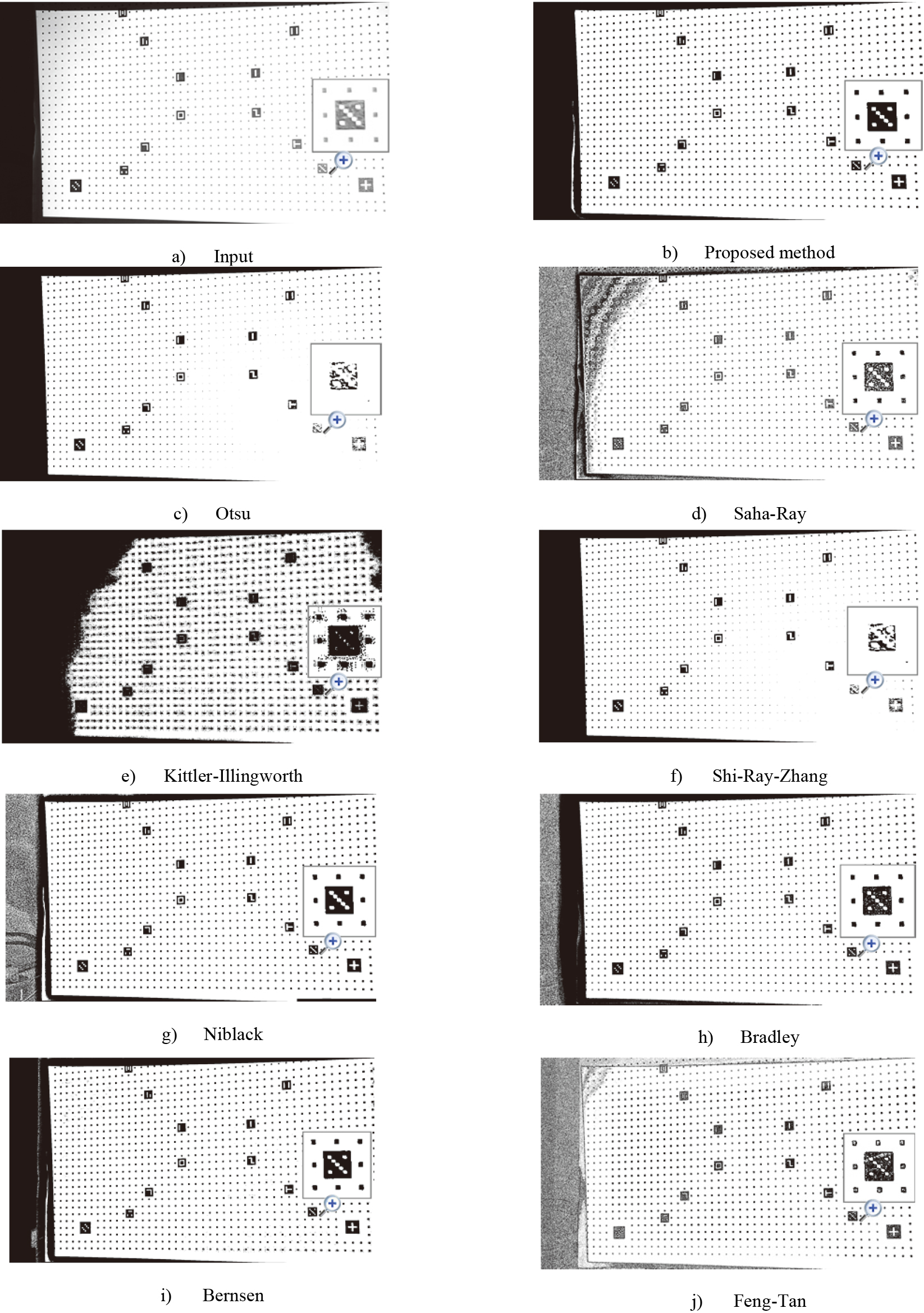

The key thing in calculating the histogram $H_{i,j+1}$ of pixel ( $i$ , $j+1$ ) is that we do not need to increment or decrement all intensities of the whole sub-image, while we just remove (decrement) the first column histogram $H_{j}$ from the previous histogram $H_{i,j}$ and add (increment) new column histogram $H_{j+1+r}$ .

Figure 6.

The comparison of image binarization algorithms on the sample with non-uniform illumination.

This way the algorithm complexity is $O$ (1) because we have:

•

One increment and one decrement for each column in histogram $H_{j}$

•

256 decrements while removing column histogram $H_{j}$ from histogram $H_{i,j+1}$ 256 increments while adding a column histogram $H_{j+1+r}$ to histogram $H_{i,j+1}$

•

Average 128 checks for median and 2 subtractions and 2 additions of the histogram for the mean value.

3.3 Determination of whether a pixel belongs to an object or background

Based on the global median, median, and average intensity of the sub-image, sensitivity function (2), and pixel intensity itself, we use the following formula to evaluate whether pixels belong to the object or background. The relative ratio of these parameters depends on the intensity of reflection. To cover the widest possible range of reflection, from small to large, we use the function:

$\displaystyle\textit{DiffRef}\left(P\right)=0.7+\frac{0.25}{1+e^{-\frac{P-150}% {20}}}$ (2)

Figure 7.

The results of the proposed method on three objects with markers. The left column presents objects with markers, while the second column presents the results of the proposed method.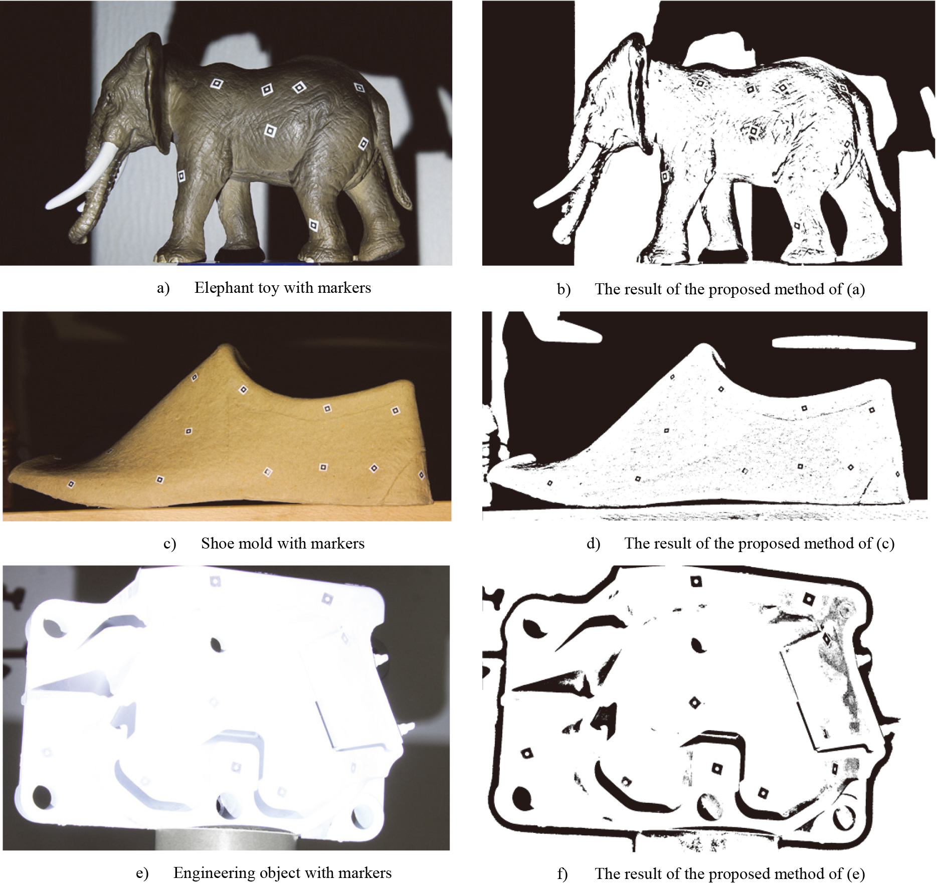

For each value from 0 to 255, the function calculates the coefficients of sensitivity to reflection. Local reflection correlates with the difference between the pixel and the mean intensity value of the sub-image of the pixel $P$ (Fig. 4). Hence, the DiffRef function presents the distribution in the percentage of how much the pixel $P$ should be lower than the mean intensity value of the sub-image of the pixel $P$ .

The proposed determination is shown in equation:

$\displaystyle B\left(P\right)=\left\{\begin{array}[]{cc}&P<\textit{DiffRef(% mean)}\ast\textit{mean}\\ 0,&\textit{or}\\ &\left|\textit{median}-\textit{globalMedian}\right|<10\\ {255,}&\textit{else}\end{array}\right.$

where mean is the mean intensity value of the sub-image of the pixel $P$ , median is the median intensity value of the same sub-image and globalMedian is the median value of the whole image.

Figure 8.

The results of the proposed method on a dataset from the DIBCO public platform.

Figure 9.

3D scanner calibration plane – light reflection, a result of the mobile 3D scanning.

The parameters 20 in Eq. (2) and parameter 10 in Eq. (3.3) have been set based on experience and a lot of testing. Based on the calculation of contrast and non-uniform illumination around markers, these parameters can be further improved or approximated by a function using contrast and brightness as inputs parameters. This will be a part of future work.

4. Results and comparison with other methods

The following figure (Fig. 5) shows a comparison with other image binarization methods in the case of a calibration image of our mobile 3D scanning system. Some of these methods do not give satisfactory results: Otsu, Saha-Ray, Kittler-Illingworth, Shi-Ray-Zhang, and Feng-Tan. Namely, the mentioned methods result in noisy regions of markers. In that situation, it is difficult to determine the markers in real-time because corner detection methods yield too many corners while line detection methods yield many dashed parts.

Compared to mentioned methods, Niblack, Bradley, and Bernsen provide quality results in our application. In the Niblack case, there is a problem in terms of large execution time (Table 1). Regarding Bradley and Bernsen, these methods are not time-consuming compared to our method and their parameters can be further adjusted such that a large set of problems can be solved by applying them.

In this sense, as we mentioned, our method can be considered as an adaptive extension of the Bradley method with additional effort in the flexible parameter setting. This extension consists of the DiffRef function and usage of the difference of median and global median values. Adaptive parameter setting is the main contribution of the proposed method, especially considering that the method can be used in standard applications.

Additional comparisons of the same methods are given in figure (Fig. 6). This is an example with included non-uniform illumination. It is evident that the proposed method does not include too many small regions what is important for the algorithmic complexity of the algorithm of connected components algorithm.

The following is an example with the results of the proposed method on three objects with markers (Fig. 7). The left column presents objects with markers, while the second column presents the results of the proposed method. We have also used these examples in table (Table 1) where the number of found markers is given.

The following figure (Fig. 8) shows the results of the proposed method in the case of a historical document. The samples belong to the public database DIPCO2016 (https://vc.ee.duth.gr/h-dibco2016/benchmark/).

Using the same parameters as in the previous example of the calibration plane (sub-image size is set according to (1)), the proposed method results in cleartext. This means that the proposed method avoids small noise regions while still being sensitive enough to keep larger regions as a whole.

The following figure (Fig. 9) shows the result of our mobile 3D scanning system which consists of a mobile phone and projector. The mobile phone used in this paper was Samsung Galaxy S8 with 8 processors, and the projector was the Optoma PK301 pico projector with a native resolution of 854 $\times$ 480 pixels and 100 ANSI lumens under power.

In this example, we show the importance and impact of the image binarization method on the final scanning result, a 3D point cloud. We applied two different image binarization setups and obtained two binarization images (Fig. 9a and b). The left figure (Fig. 9a) is the result of the proposed method, where the sub-image size is set according to (1). The right image is also the result of the proposed method, but the sub-image size is twice as large as in the case of the left image.

Twice the sub-image size results in larger (spilled) markers. Thus, the centers of these markers as connected regions differ from the centers of the markers of the left image. Positions in the 3D space of these markers and triangulated surfaces of both cases are shown in figures Fig. 9c and d respectively. Based on those 3D positions we fit the 3D calibration plane and get the scanner calibration parameters.

Figure 9e shows the distribution of difference of the two surfaces of the calibration plane (Fig. 9c and d). The final impact of different image binarization methods is shown in figure (Fig. 9f). The image contains the distribution of the difference of two triangulated 3D point clouds obtained by our 3D mobile scanning system where the first point cloud is based on the binarization image (Fig. 9a) and the second point cloud on the binarization image (Fig. 9b). These results show the importance of the binarization method is in calculating the calibration parameters of the proposed mobile scanner. The goal is to obtain the most accurate 2D initial values for calculating the 3D position of the marker, so the accuracy of the proposed method is extremely important to us.

The next table (Table 1) contains the computation time for the same examples. The PC we used for the calculation has an Intel(R) Core (TM) i7-8700K processor with 3.7 GHz. The system is Windows 10 and the compiler we used is Microsoft Visual Studio 2019 compiler /O2.

Table 1
The computational cost for example in Fig. 6

Methods	Time (s)
Saha-Ray	99.53
Niblack	82.07
Otsu	0.5333
Shi-Ray-Zhang	26.10
Kittler-Illingworth	0.9961
Bradley	0.30
Bernsen	0.48
Feng-Tan	0.49
Proposed	0.49

The most important performance parameter for the proposed method is the number of markers found. The table below lists the number of markers found for nine different methods on the examples in Fig. 6. It is evident from the results that the application of the proposed method is justified.

Figure 10.

Referent images for calculating F-Measure and NRM measure for images from Fig. 7.

Table 2

The number of markers found for the examples in Fig. 7

Methods	Found markers (%)
Saha-Ray	74.2
Niblack	89.9
Otsu	60.1
Shi-Ray-Zhang	53.8
Kittler-Illingworth	4.3
Bradley	69.2
Bernsen	75.6
Feng-Tan	0
Proposed	89.8

Since we have given a result of the application of the proposed method in the case of a historical document (Fig. 8), we bring the mean values of the F-Measure and Negative Rate Metric (NRM) [35] that apply in such cases (Table 3).

Table 3

F-Measure and NRM measures for the examples from Fig. 8

Method	F-measure	NRM
Saha-Ray	0.490806	0.104832
Niblack	0.308690	0.105435
Otsu	0.887279	0.050606
Shi-Ray-Zhang	0.891047	0.047096
Kittler-Illingworth	0.397663	0.070684
Bradley	0.567855	0.039610
Bernsen	0.280638	0.122043
Feng-Tan	0.822008	0.131901
Proposed	0.689214	0.166805

We also calculated the mean values of the same measures on examples with markers from the figure (Fig. 7). The values have shown in the table below.

Table 4

F-Measure and NRM measures for the examples from Fig. 7

Method	F-measure	NRM
Saha-Ray	0.022811	0.238341
Niblack	0.013333	0.253060
Otsu	0.003566	0.452885
Shi-Ray-Zhang	0.003924	0.452836
Kittler-Illingworth	0.008267	0.555613
Bradley	0.008679	0.338135
Bernsen	0.015608	0.267318
Feng-Tan	0.036854	0.325283
Proposed	0.030055	0.212576

The reference images for calculating the measures in the table above are shown in Fig. 10 where the background is completely white.

In our opinion, these measures do not make much sense in this case because the actual background varies between white and black and thus affects the calculated values.

5. Discussion

The obtained results show the success of the proposed method in conditions of strong reflection and uneven illumination. In most cases, it was sufficient to use the method with the fixed sub-image kernel size. An adaptive sub-image size calculation is needed in cases where a previous call with a fixed size is not good enough. This, of course, saves extra time. We assume that methods based on deep learning give equal or better results, but in that case, time execution does not allow execution in applications such as a mobile 3D scanner. The calculation of measures such as F-measure and Negative rate metric (NRM) only makes sense in cases where images that contain markers have a consistent background, only black or only white.

6. Conclusion

This paper outlines an image binarization method with the main purpose of finding markers in a mobile 3D scanning system. As well known, different applications and conditions imply different settings of existing binarization methods. We are aware that finding markers with 100% success is not realistic and that improvements to some other methods can give the same or even a higher number of found markers. Nevertheless, we have shown that in cases of strong light reflection and non-uniform illumination, our method is robust and fast enough to be used in real-time applications such as mobile scanners.

7. Future work

In future work, we plan to remove the constant values set by testing (Function (2), Algorithm 1). Based on contrast calculation and non-uniform illumination around markers we will try to design a new function that should improve the current result regarding finding markers. Also, the functionality will be applied in the binarization of historical documents and there we expect more progress.

Footnotes

Acknowledgments

This work was supported by the Croatian Science Foundation [HRZZ-IP-2018-01-6774].

References

Benamara

Val-Calvo

Álvarez-Sánchez

Díaz-Morcillo

Ferrández-Vicente

Fernández-Jover

, et al. Real-time facial expression recognition using smoothed deep neural network ensemble. Integr Comput Aided Eng. 2020 Dec 21; 28(1): 97-111.

Bernsen

. Dynamic Thresholding Of Grey-Level Images. In: Proceedings – International Conference on Pattern Recognition, 1986.

Bhattacharyya

. On a measure of divergence between two statistical populations defined by their probability distributions. Bull Calcutta Math Soc. 1943; 35: 99-109.

Bradley

Roth

. Adaptive thresholding using the integral image. J Graph Tools. 2007 Jan 30; 12(2): 13-21.

Chen

Toyoura

Terada

Mao

. Image-based textile decoding. Integr Comput Aided Eng. 2021 Mar 5; 28(2): 177-90.

Van Crombrugge

Penne

Vanlanduit

. People tracking with range cameras using density maps and 2D blob splitting. Integr Comput Aided Eng. 2019 Apr 28; 26(3): 285-95.

Delmas

Gee

. Stereo camera visual odometry for moving urban environments. Integr Comput Aided Eng. 2019 Apr 28; 26(3): 243-56.

Eyupoglu

. Implementation of Bernsen’s Locally Adaptive Binarization Method for Gray Scale Images. J Sci Technol. 2017; 7(2).

Feng

M-L

Tan

Y-P

. Contrast adaptive binarization of low quality document images. IEICE Electron Express. 2004; 1(16): 501-6.

10.

García

Fernández-Sotos

Vicente-Querol

Lahera

Rodriguez-Jimenez

Fernández-Caballero

. Design of reliable virtual human facial expressions and validation by healthy people. Ferrández

Andina

Fernández

, editors. Integr Comput Aided Eng. 2020 May 20; 27(3): 287-99.

11.

Halima

Laferté

J-M

Cormier

Fougères

A-J

Dillenseger

J-L

. Depth and thermal information fusion for head tracking using particle filter in a fall detection context. Integr Comput Aided Eng. 2020 Feb 27; 27(2): 195-208.

12.

Hamreras

Boucheham

Molina-Cabello

Benítez-Rochel

López-Rubio

. Content based image retrieval by ensembles of deep learning object classifiers. Ferrández JM, Andina D, Fernández E, editors. Integr Comput Aided Eng. 2020 May 20; 27(3): 317-31.

13.

Ismail

Sheikh Abdullah

SNH

Fauzi

. Statistical Binarization Techniques for Document Image Analysis. J Comput Sci. 2018 Jan 1; 14(1): 23-36.

14.

Kesiman

MWA

Prum

Burie

J-C

Ogier

J-M

. An initial study on the construction of ground truth binarized images of ancient palm leaf manuscripts. In: 2015 13th International Conference on Document Analysis and Recognition (ICDAR), IEEE; 2015. pp. 656-60.

15.

Khurshid

Siddiqi

Faure

Vincent

. Comparison of Niblack inspired binarization methods for ancient documents. In: Document Recognition and Retrieval XVI, 2009.

16.

Kittler

Illingworth

. Minimum error thresholding. Pattern Recognit. 1986 Jan; 19(1): 41-7.

17.

Lins

Silva de FP e

de Almeida

. Binarizing complex scanned documents. In: 2015 13th International Conference on Document Analysis and Recognition (ICDAR). IEEE; 2015s, pp. 56-60.

18.

Mitianoudis

Papamarkos

. Document image binarization using local features and Gaussian mixture modeling. Image Vis Comput. 2015; 38.

19.

Mustafa

Aziz

Khairunizam

Ibrahim

Shahriman

Razlan

. Review of different binarization approaches on degraded document images. In: 2018 International Conference on Computational Approach in Smart Systems Design and Applications, ICASSDA 2018, 2018.

20.

Naranjo

Santos

Garmendia

. A convolution-based distance measure for fuzzy singletons and its application in a pattern recognition problem. Integr Comput Aided Eng. 2020 Dec 21; 28(1): 51-63.

21.

Niblack

. An introduction to digital image processing. Strandberg Publishing Company Birkeroed, 1985.

22.

Otsu

. A threshold selection method from gray-level histograms. IEEE Trans Syst Man Cybern. 1979 Jan; 9(1): 62-6.

23.

Papamarkos

Gatos

. A new approach for multithreshold selection. Comput Vision, Graph Image Process Model Image, Process. 1994; 56(5): 357-70.

24.

Pérez-Hurtado

Martínez-del-Amor

MÁ

Zhang

Neri

Pérez-Jiménez

. A membrane parallel rapidly-exploring random tree algorithm for robotic motion planning. Integr Comput Aided Eng. 2020 Feb 27; 27(2): 121-38.

25.

Perreault

Hebert

. Median filtering in constant time. IEEE Trans Image Process. 2007 Sep; 16(9): 2389-94.

26.

Pratikakis

Zagoris

Barlas

Gatos

. ICDAR2017 Competition on Document Image Binarization (DIBCO 2017). In: 2017 14th IAPR International Conference on Document Analysis and Recognition (ICDAR). IEEE; 2017. pp. 1395-403.

27.

Roe

Mello

CAB

. Thresholding color images of historical documents with preservation of the visual quality of graphical elements. Integr Comput Aided Eng. 2018 May 17; 25(3): 261-72.

28.

Rostami

Neri

Epitropakis

. Progressive preference articulation for decision making in multi-objective optimisation problems. Integr Comput Aided Eng. 2017 Sep 5; 24(4): 315-35.

29.

Saha

Ray

. Image thresholding by variational minimax optimization. Pattern Recognit. 2009 May; 42(5): 843-56.

30.

Santiago

DJC

Ren

Cavalcanti

GDC

Jyh

. Efficient 2 × 2 block-based connected components labeling algorithms. In: 2015 IEEE International Conference on Image Processing (ICIP). IEEE; 2015. pp. 4818-22.

31.

Sauvola

Pietikäinen

. Adaptive document image binarization. Pattern Recognit. 2000 Feb; 33(2): 225-36.

32.

Shi

Ray

Zhang

. Shape based local thresholding for binarization of document images. Pattern Recognit Lett. 2012 Jan; 33(1): 24-32.

33.

Singh

Sharma

Ghosh

Mittal

. Adaptive bina-rization of severely degraded and non-uniformly illuminated documents. Int J Doc Anal Recognit. 2014 Dec 30; 17(4): 393-412.

34.

Siqueira

Santana

Macedo

Figueiredo

Gokhale

Bastos-Filho

. Simplified binary cat swarm optimization. Integr Comput Aided Eng. 2020 Dec 21; 28(1): 35-50.

35.

Sulaiman

Omar

Nasrudin

. Degraded historical document binarization: A review on issues, challenges, techniques, and future directions. J Imaging. 2019 Apr 12; 5(4): 48.

36.

Tensmeyer

Martinez

. Document image binarization with fully convolutional neural networks. In: 2017 14th IAPR International Conference on Document Analysis and Recognition (ICDAR). IEEE; 2017, pp. 99-104.

37.

Thurnhofer-Hemsi

López-Rubio

Roé-Vellvé

Molina-Cabello

. Multiobjective optimization of deep neural networks with combinations of Lp-norm cost functions for 3D medical image super-resolution. Ferrández JM, Andina D, Fernández E, editors. Integr Comput Aided Eng. 2020 May 20; 27(3): 233-51.

38.

Tran

M-T

Q-N

Lee

G-S

. Binarization of music score with complex background by deep convolutional neural networks. Multimed Tools Appl. 2021 Mar 3; 80(7): 11031-47.

39.

Kim

Yang

Lee

. Binarization of degraded document images based on hierarchical deep supervised network. Pattern Recognit. 2018 Feb; 74: 568-86.

40.

Wang

Zhang

Gou

Paul

Neri

Rong

, et al. Multi-behaviors coordination controller design with enzymatic numerical P systems for robots. Integr Comput Aided Eng. 2021 Mar 5; 28(2): 119-40.

41.

Wen

Sun

. A new binarization method for non-uniform illuminated document images. Pattern Recognit. 2013 Jun; 46(6): 1670-90.

42.

Zhang

Zhu

Jiang

Neri

. Geometry based three-dimensional image processing method for electronic cluster eye. Integr Comput Aided Eng. 2018 May 17; 25(3): 213-28.

43.

Yan

Zhang

Xie

. An optimizer ensemble algorithm and its application to image registration. Integr Comput Aided Eng. 2019 Sep 11; 26(4): 311-27.

44.

Liu

Srihari

. Document image binarization based on texture features. IEEE Trans Pattern Anal Mach Intell. 1997 May; 19(5): 540-4.

Image binarization method for markers tracking in extreme light conditions

Abstract

Keywords

1. Introduction

1.1 Motivation

1.2 Background and applications

2. Related work

3. Proposed method

Table 1 The computational cost for example in Fig. 6

6. Conclusion

7. Future work

Footnotes

Acknowledgments

References

Table 1
The computational cost for example in Fig. 6