
Abstract
Safe navigation at sea is more important than ever. Cargo is usually transported by vessel because it makes economic sense. However, marine accidents can cause huge losses of people, cargo, and the vessel itself, as well as irreversible ecological disasters. These are the reasons to strive for safe vessel navigation. The navigator shall ensure safe vessel navigation. He must plan every maneuver and act safely. At the same time, he must evaluate and predict the actions of other vessels in dense maritime traffic. This is a complicated process and requires constant human concentration. It is a very tiring and long-lasting duty. Therefore, human error is the main reason of collisions between vessels. In this paper, different reinforcement learning strategies have been explored in order to find the most appropriate one for the real-life problem of ensuring safe maneuvring in maritime traffic. An experiment using different algorithms was conducted to discover a suitable method for autonomous vessel navigation. The experiments indicate that the most effective algorithm (Deep SARSA) allows reaching 92.08% accuracy. The efficiency of the proposed model is demonstrated through a real-life collision between two vessels and how it could have been avoided.
Introduction
The development of artificial intelligence (AI) has become an essential trend in many applications. The AI can be applied to a wide range of tasks and systems, see e.g. [1, 2, 3, 4, 5, 6, 7, 8, 9, 10, 11, 62, 64, 65]. It is essential because it solves routine tasks and could carry out monitoring of vital processes. Medicine is one of the most attractive fields for AI, see [3, 4, 5, 11, 64] for exciting applications. This is because medicine generates huge amounts of visual and numerical data. Recently, the theory of artificial intelligence has been developed (e.g. [10, 65]), and new application fields are arising: emotion recognition [6], information fusion [7], time series analysis [8, 63], etc. In this paper, we extend the use of AI for ship collision avoidance through a reinforcement learning approach.
Nowadays, more than ever before, cargo shipping has become vital to the global economy. This leads to maritime congestion and makes maritime traffic difficult and dangerous. Vessels are trying to carry the cargo as fast as possible and cost-effective. The main challenge is to operate a large and loaded vessel safely while ensuring best maritime practices for navigation. It is crucial because vessel collisions cause to loss of human life, property, and vessels. This problem must be solved by providing navigators with timely and relevant navigational information. The navigational information could ensure right decisions. On the other side, the usage of navigational information is limited by the navigator’s perception and experience. Therefore, navigational information by itself is not sufficient to avoid a collision between vessels. The safe voyage of a vessel depends on the experience and reaction of the navigator.
Navigators are required to carry out their duties personally on the vessel bridge. This rule helps to ensure a safe vessel voyage. Recently, technologies have significantly improved safety and reduced the risk of collisions. The primary technology that ensures safe navigation is radar. Radar uses electromagnetic waves to calculate the position of vessels or other obstacles. Otherwise, radar does not by itself ensure the safe vessel navigation. The radar uses the Automatic Radar Plotting Aid (ARPA) [12] to reduce the risk of collision. ARPA is an excellent tool for calculating and predicting dangerous maneuvres of vessels. The main problem with this calculation is that the maneuvering situation can change at any time. However, ARPA is the most effective tool when the speed and course of vessels are constant.
Technologies for autonomous vessel navigation are being developed. This is a key direction in the development of various artificial intelligence-based approaches. An autonomous vessel could significantly reduce the cost of vessel maintenance and operation. In addition, it could help to solve problems of recruitment or crew management. However, all these costs cannot be reduced without ensuring a safe vessel voyage. In addition, the use of autonomous vessel technologies could save fuel. This could be done by continuously analyzing and recalculating the vessel voyage parameters (weather, maneuvering actions, etc.) and adjusting the vessel route and the main engine load. On the other side, autonomous technologies could significantly improve the quality of life at sea. It could be achieved by reducing the number of crew members and creating better living spaces. The same strategy could be applied to maximize cargo space [13]. However, autonomous vessels face a variety of problems (legal [14], technical [13]). These problems must be resolved before autonomous vessel technology would be applied. A number of projects have been launched to address the problems of autonomous shipping; for example, the Yara Birkeland electric autonomous vessel [15], the MUNIN research project [16], and the DIMECC “One Sea” Consortium [17].
To assess the maneuvring situation, various factors need to be considered. For example, geographical or hydro-meteorological conditions are important for safe vessel maneuvering. As mentioned before, human error is the main cause of accidents at sea. The navigators must find the safest way to navigate in maritime traffic. Therefore, it is essential to discover the most suitable algorithm to maintain alertness and help to navigate.
This paper discloses the ideas of applying the different reinforcement learning strategies. It extends and generalizes the results of [18]. The various algorithms operate through an agent that performs the suggested maneuvers.
Related work
In recent years, various autonomous vehicles have been under development. The main aim of autonomous vehicles is to save human lives. This applies primarily to land transport. However, it is also essential for the maritime industry to avoid collisions at sea, to solve crew hiring, vessel maintenance problems, and voyage time limitations.
Many different methods were created to avoid the collision, see [12, 19, 20]. The methods used to avoid collisions vary widely, depending on the formulation of the problem – dynamic games theory [21], dynamic programming [22], maze routing algorithm [23], fast marching method [24], genetic algorithm [25, 26], cooperative path planning algorithm [27], artificial potential field [28], the fuzzy logic-based method [29], evolutionary algorithms [30] and ant colony optimization [31].
The application of automated navigational aids reduces the risk of collision. To improve the safety of maritime navigation, intelligent decision-making tools and systems must be able to detect anomalies or dangerous situations. The case-based reasoning system is proposed in [35]. This system is created to solve the vessel turning problems. It was applied for ocean navigation and collision. The idea of case-based reasoning lies in retrieving past solutions that are similar to the current situation and adapting them for the proper decision. The Radar filtration algorithm is proposed in [37]. It helps the vessel traffic service officer gauge the degree of collision risk around a particular vessel. The software displays the vessel’s list based on their degree of collision severity.
Some studies attempted to apply the Artificial Neural Networks (ANN) model for safe marine navigation. These models learn the actions of navigation officer and predict maneuvers [32]. Also, [33] tried to predict the effect of waves on the vessel yaw motion. However, the biggest issue for ANN is to predict the vessel collision. The vessel collision analysis proposed in [34] is a simplified analytical approach. The authors used the interaction between the deformation on the striking and the struck vessels. This approach involves experiments, numerical simulations, and simplified analytical methods. It can be applied from the local element down to the small ship level. The study [38] combined a fuzzy inference system with an expert system in the collision avoidance system. A multi-layer perceptron neural network is applied to the collision avoidance system to make up for fuzzy logic. The study [39] presents two approaches for anomaly detection. It has been proposed to analyze the network traffic in cloud communications. The analysis was based on Synergetic Neural Networks and catastrophe theory.
Machine learning found application in [36], where the marine traffic anomaly detection by the combination of the DBSCAN clustering algorithm (Density-Based Spatial Clustering of Applications with Noise) with k-nearest neighbors analysis among the clusters and particular vessels has been proposed. Probabilistic forecasting of maritime traffic is proposed in [42]. A knowledge-assisted methodology is used for maritime traffic forecasting. It is based on a vessel’s waterway pattern and motion behavior. The DBSCAN algorithm was applied to extract the vessel’s waterway pattern. The seaway model was used to predict the position of the opposing vessel based on the route extraction method proposed in [41]. The regression model combined with the dead reckoning model has been trained. Machine learning algorithms incorporate both the vessel’s waterway pattern and motion behavior knowledge to get a set of probable coordinates in [43].
In recent years, Deep Learning (DL) found attention in marine traffic patterns or anomalies, too [45]. This technology seems to have broad applications in further analysis of marine geospatial data.
Our paper considers deep reinforcement learning as a part of the autonomous vessel navigation system. Deep reinforcement learning combines artificial neural networks with a framework of reinforcement learning. As a result, software agents learn how to reach their goals. This is a new stage in vessel navigation research.
The idea of an agent for navigation
Navigation in marine traffic is a complicated task, even for a human. This study aims to apply the different reinforcement learning (RL) algorithms acting as agents in maritime traffic. Reinforcement learning (RL) [46, 47] is the framework for solving various control tasks. The RL algorithms can process complex data and learn from data patterns. It could be achieved by rewarding the right decisions and maximizing rewards. This allows the RL algorithm to predict wrong decisions and avoid negative rewards. At first, the RL agent must avoid collision with an obstacle. The second aim is to reach the position of the destination. The agent is trained to act in some area (environment) of marine traffics. The environment contains participants in the maritime traffic, including possible moving obstacles. The maritime traffic area is interpreted in this case as a fixed-size grid structure with a dynamic obstacle. The agent tries to learn the acting in the grid with one obstacle. Such limitation to one obstacle simplifies the task. However, such evaluation of the situation is usual in everyday marine navigation because decisions are made according to the most risky obstacles.
Thus, like the navigator on the vessel, the RL algorithms allow the agent to learn about the current state in the surrounding area and to decide about the possible action. So, the agent or vessel should avoid obstacles and make safe maneuvering depending on the situation. The agent must reach the point of destination. This point of destination in the real environment area could be expressed as a turning waypoint. This turning point is a part of the route between two ports. Usually, turning waypoints are preplanned in advance before the voyage starts. The agent must start from one turning point and safely reach the next turning point.
Therefore, the main idea is that the agent learns actions based on the environment. We propose a specific approach for assessing and applying trained agents. The learning environment is the same marine traffic on a particular time scale. For example, the time scale could be 1 min, 3 min, or 6 min. it depends on the concrete situation – distance and speed between vessels. Such an approach is common in marine navigation because all predictions (for example, on Radars) are based on such calculations on different time scales.
The applied reinforcement algorithms
In this paper, four different algorithms were used to navigate the vessel around other vessels or obstacles. According to the restrictions mentioned above, the RL algorithms simulate vessel control. Thus, the non-human expert can be used to learn the maneuver in the vicinity of other vessels and obstacles. The reward system was used in the environment of learning. The agent is rewarded when the vessel reaches the point of destination in the considered area. In this area, the agent (in our case – the vessel) tries to learn to maneuver around obstacles. The agent has two primary purposes: to achieve the destination position and not appear in the same position with obstacles simultaneously. In the modeling and training, the obstacle moves like other usual vessels in marine traffic. Thus, the agent should plan the moves in a dynamic environment.
In this paper, the possibilities of applying different reinforcement learning algorithms to control the vessel are investigated. The chosen four methods represent Model-Based (Monte Carlo) and Model-Free (algorithm of the Q-learning family) reinforcement learning algorithms. The deeper analysis shows the Model-Free potential, especially of the Deep SARSA.
Q-learning.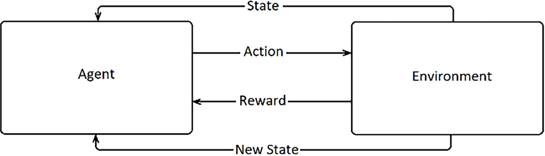
These are four different algorithms:
The RL algorithm is intended to solve a Markov Decision Process (MDP) – a discrete-time stochastic control process. As shown in Fig. 1, in MDP we deal with:
A set of states. The states represent the agent’s all possible locations in the environment. A set of actions. The set of actions represents all possible actions that the agent could take in the environment. Transition probabilities. The probability of success of the agents’ decision. Rewards. The value of the reward depends on the agent’s specific state. A discount factor. The factor’s purpose is to diminish the value of future rewards compared to instant rewards.
A policy is defined as a mapping between the state-action and the probability of taking action in a state. The agent’s purpose is to learn the optimal policy, and this policy must ensure optimal actions in any given state.
Q-learning is model-free and belongs to reinforcement learning methods. It was proposed in [48]. It is an active reinforcement method, and its agent’s policy or Q-table is generated on the fly. This Q-table uses state-action pairs to index a Q-value. This value is described as an expected discounted future reward for taking action in a particular state. Thus, every state has an assigned value. The Q-learning algorithm exploits off-policy control to maximize the expected value. It allows isolating the deferral policy from the learning policy. The action is selected by the Bellman optimal equations and the
In Q-learning, a lookup table (Q-table) of maximum expected rewards is made at each state. The Q-table guides the agent for the best action at each state. In our case, the environment initially generates an obstacle at a random place in every episode. The random generation of obstacles makes learning tasks close to real situations.
SARSA algorithm
The second algorithm applied is SARSA (State – Action – Reward – State – Action) [49, 50]. In the same way as the Q-learning algorithm, SARSA tries to explore the grid area. Actions are the same: up, down, right, and left. The episode starts with constant rewards until the goal position is reached. The SARSA algorithm explores different options to discover the best solution based on the optimal policy. The policy is generalized by using iteration by the Temporal-Difference learning (TD). This is used in the evaluations or prediction part.
Contrary to the Q-learning algorithm, the first step of SARSA is to learn an action-value function comparatively to a state-value function. The episode consists of an alternating sequence of states and state-action pairs. As with all on-policy methods, SARSA continually estimates the action-value for the current behavior policy.
Monte Carlo algorithm
Monte Carlo algorithm learns from episodes without prior knowledge of MDP (the states, actions, rewards, etc.) transitions. This method is essentially a random sampling from the environment [51]. The deficiency of Monte Carlo lies in the fact that the return of the episode could be calculated only when the episode expires. Thus, this algorithm lacks the ability to update the reward after every action. The Monte Carlo goal is to estimate value-action (Value|State, Action) or value-function (Value|State) from episodes of experience under a random policy. After every performed episode, Monte Carlo acquires an experience that is represented as the sequences of states, actions, and rewards. This experience is determined by simulation of interaction with the environment.
At the start, Monte Carlo initializes the policy and state-value function [52]. After this step, it starts generating an episode considering the current policy. The state’s status is saved after every episode. The return is added to the list of returns, and the returns are averaged overall. The calculated average is used as the state value. This step is repeated until it finds the optimal policy.
The Monte Carlo method must be applied cautiously because the end of the episode is not assured for all policies.
Deep SARSA algorithm
AI in recent years has made significant progress because of the development of machine learning, especially deep learning (DL) tools. For example, the DeepMind team has recently successfully trained an agent using a Deep RL (DRL) algorithm to game Go, eventually defeating a human professional player. The DRL is an important research field in machine learning and consists of two parts: deep learning (DL) and reinforcement learning (RL) [53, 54]. Here the reinforcement signal was used to critique the action and gain experience from the environment through several trials and errors. DRL is based on a neural network. The neural network tries to predict the action based on the various environment [55, 56]. Thus, the neural network is getting states as input. The suggestion of action is the output of the neural network. This action is from the set of possible actions.
Deep SARSA is exploiting the SARSA on-policy RL algorithm together with the deep learning method. It allows to estimate state action values and build an optimal policy for an agent. For each episode, the agent starts from steps based on the epsilon-greedy policy. The Deep SARSA uses two methods to achieve better results:
Experience replay technique – the tuples of the previous actions are stored into replay memory. This technique helps the agent learn and avoids oscillations or divergence in the parameters. The double estimator technique – the Double Q-learning helps determine the value of the next state to reduce overestimations.
Deep SARSA algorithm searches the future rewards by strategies. The Deep SARSA algorithm does not rely on one single best action.
In reinforcement learning, after every episode, the agent collects information about the environment. This information is used to find an optimal strategy to achieve the agent’s goals. Some learning value Epsilon should decay due to the agent’s learning. Epsilon’s value should decay across an agent’s life to have it learn and act optimally eventually [55]. Epsilon is multiplied by the real value less than 1 in every episode. This exploration is called the decaying Epsilon exploration method [58, 59]. The decay of Epsilon expresses the learning progress of the optimal strategy. Epsilon decay progress during the experiment is illustrated in Fig. 2.
All tested RL is performed in some environment. In general, the environment is any dynamic process, and this process generates data that belongs to achieving our objective. This data is of a particular size and type. The particular data of the environment is bundled into discrete packets, and it is a state of the environment. The states allow passing data to the RL algorithm at discrete time steps. In our case, the environment contains some area of marine traffics, including possible moving obstacles.
Epsilon decay progress depending on episodes.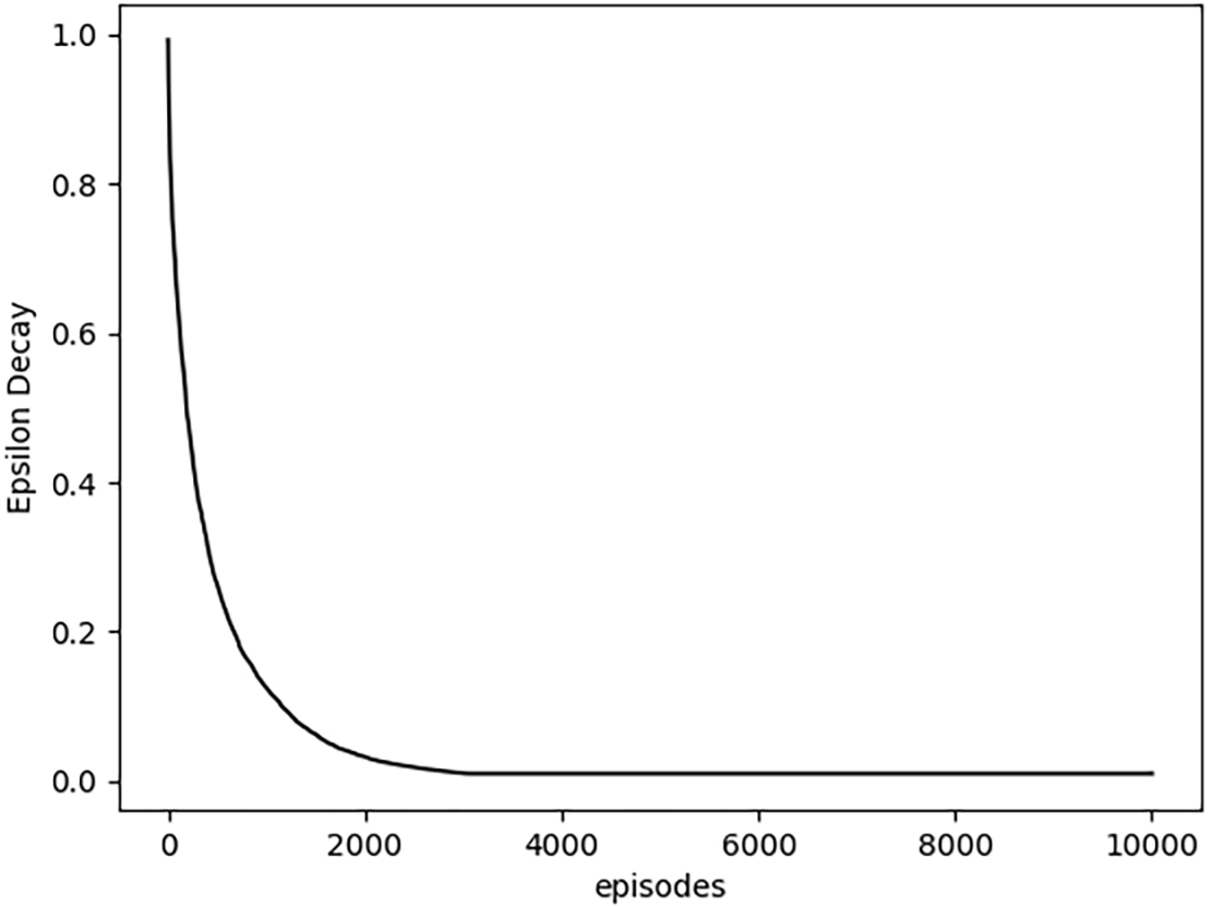
The proposed experiment was conducted on the 5
The agent acts in some environment. Let the environment consists of 25 possible positions – the grid of 5 rows and 5 columns, where the vessel spends the same time (e.g. 1 or 6 minutes). There are four possible actions of an agent: up, down, right, and left.
The examples of situations are presented in Fig. 3: (a) is the initial state, and (b) is some intermediate state. The environment is given as a square with 25 subsquares inside it. The hexagon denotes the agent. The black square denotes the destination. The rhombus denotes the obstacle. The continuous lines with arrows denote the actual direction of motion. The dotted lines with arrows denote other possible moving directions of the obstacles. The agent’s motion starts from the left upper corner and tries to reach a square (see Fig. 3). The agent starts to learn about possible actions in the environment. The trained agent should predict the next position of the moving obstacle to avoid a collision.
The training process consists of episodes. In these episodes, the agent tries to learn about the environment and solve the maneuvering/optimization problem. Therefore, the episode consists of one agent, one obstacle, and a point of destination. The main goal of the agent is to reach the destination point. The environment is dynamic. The agent and obstacle are moving continuously. Thus, the obstacle could move independently in any direction (up, down, right, and left) on the grid. Moreover, the start position of the obstacle is chosen at random in every episode. The agent is self-training to avoid obstacles and other vessels. If the agent reaches the point of the destination, it yields a reward of 1. If the agent makes a collision with an obstacle, it causes a penalty of 1 point. The agent should learn to navigate around various obstacles or other moving vessels.
Agent training: a) initial state, b) intermediate state.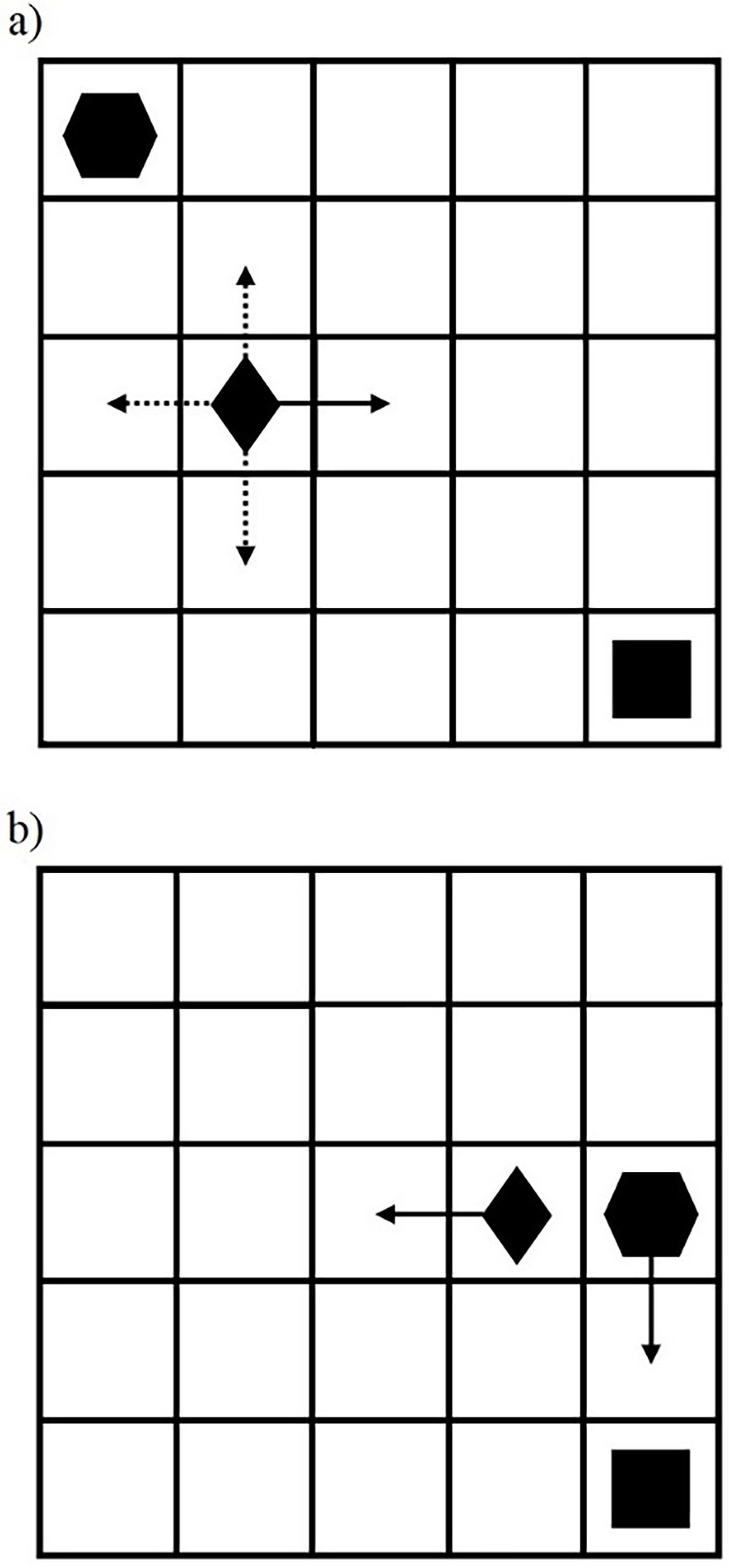
If the agent reaches the point of destination with collision, it fails to learn the episode. The agent should reach the destination point in 25 steps. Otherwise, it fails – returns
The agent must reach the destination in not more than 25 steps because of a few reasons:
the optimal strategy consists of much fewer steps than 25, the agent learning time is not wasted on hopeless strategies, 25 steps are adequate to avoid obstacles and reach the destination.
Another essential parameter that allows us to evaluate the training progress is the number of successful episodes. The results are given in Figs 4–7. During the first steps, the agent does not achieve good performance. However, the performance achieves better results with every later step.
In this paper, we performed experiments designed to provide insight into controlling the movement of agents in an unknown environment with moving obstacles. In particular, we investigate the potential of agents to safely reach their destination in a dynamic environment. The four different RL algorithms were applied to achieve this task. It is the first step in making a completely functional system for autonomous vessel navigation. The next possible step would be to make RL based decision system based on actual marine traffic data.
Agent, based on Q-learning algorithm, learning: a) after 50 episodes, b) after 100 episodes.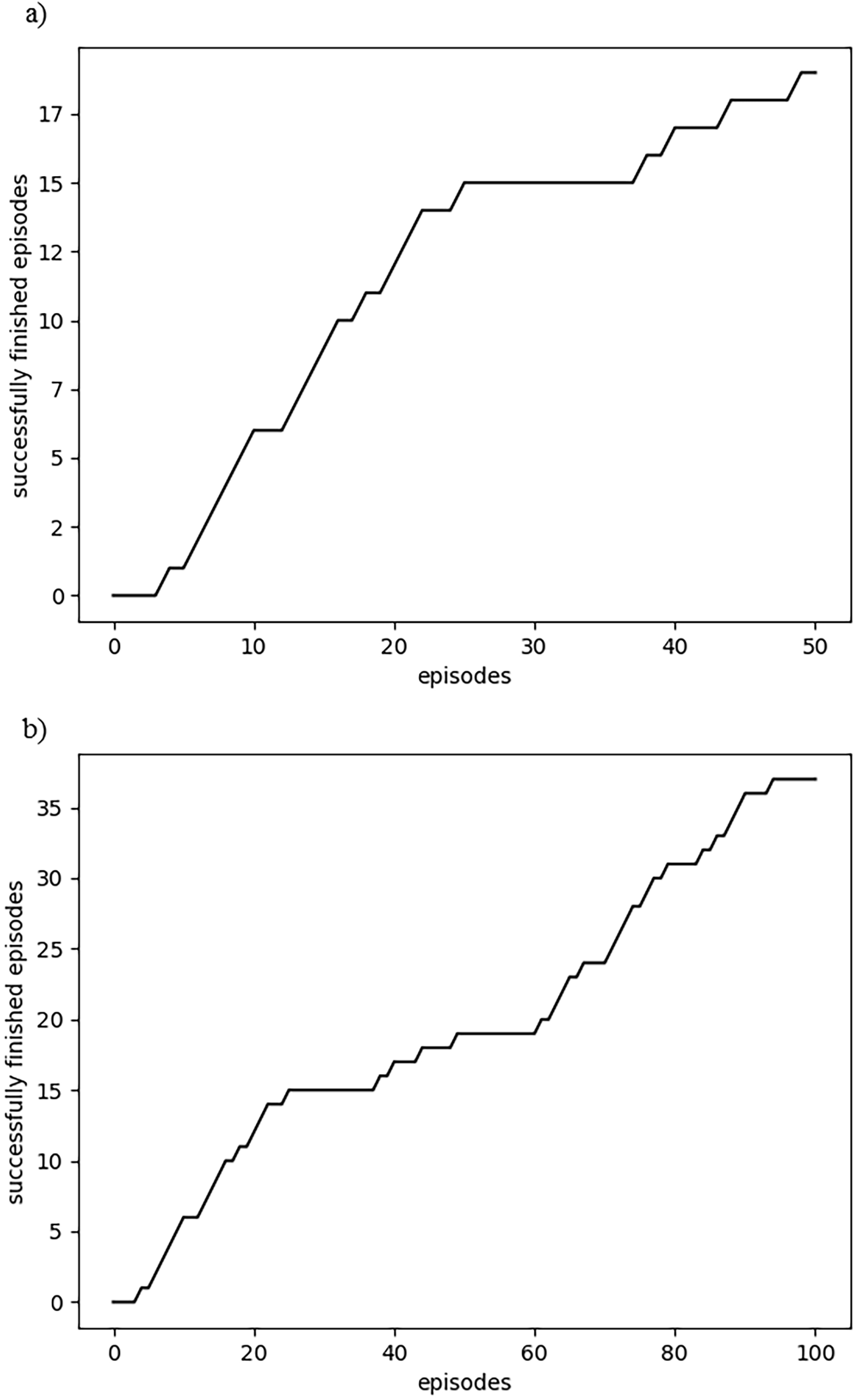
Agent, based on SARSA algorithm, learning: a) after 50 episodes, b) after 100 episodes.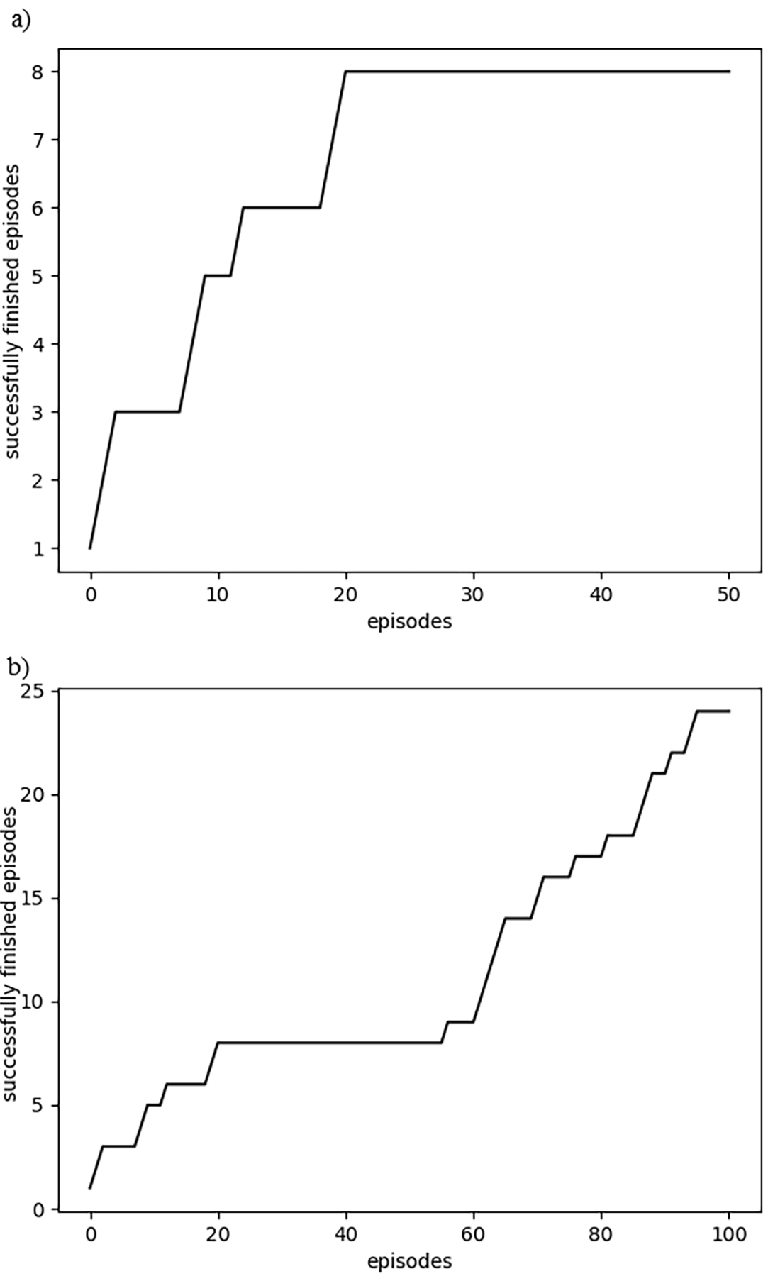
The new environment is generated on every episode. As mentioned before, the environment, corresponding to marine traffics, includes the moving obstacle. The starting position of the obstacle is chosen randomly in every episode. Moreover, the obstacle could move independently in any direction (vertical/horizontal) on every step. The agent must avoid collision with an obstacle and reach the position of the destination.
The first experiment was carried out using the Q-learning algorithm. The agent reaches 37.25% precision after 50 episodes, as shown in Fig. 4. The learning reaches 36.63% precision after 100 episodes. In our case, precision is the percent of episodes where the agent successfully reaches the point of destination. The detailed learning progress is shown in Table 1. The primary episodes last about 5 min. because the agent starts with a low experience in finding the point of destination.
A similar experiment was done using by SARSA algorithm. The agent reaches 15.69% precision after 50 episodes, as shown in Fig. 5. The learning reaches 23.76% precision after 100 episodes.
A further experiment was done using by Monte Carlo algorithm. The agent reaches 49.02% precision after 50 episodes, as shown in Fig. 6. The learning reaches 57.43% precision after 100 episodes.
Learning progress of RL algorithms
Agent, based on Monte Carlo algorithm, learning: a) after 50 episodes, b) after 100 episodes.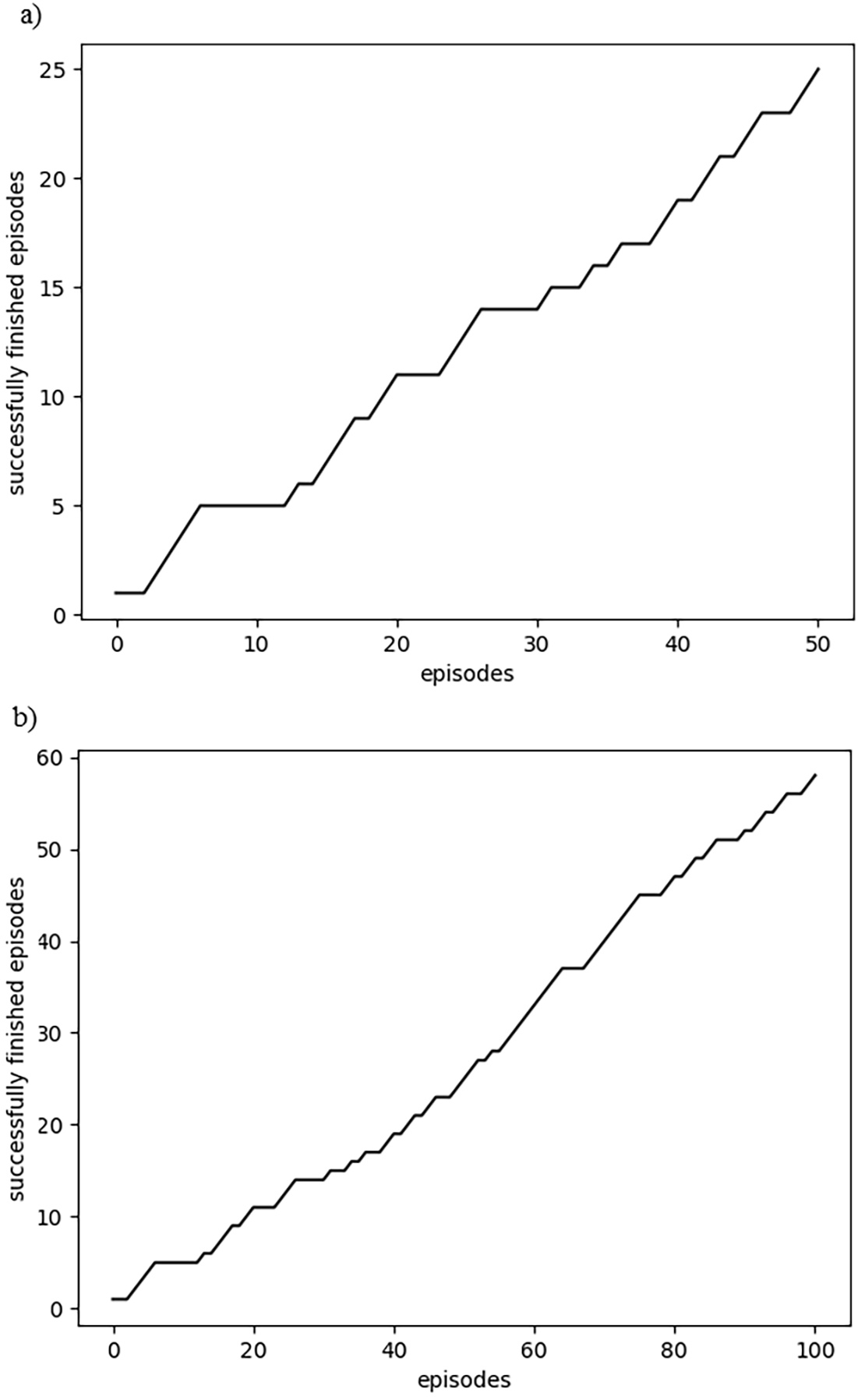
The progress of the Deep SARSA algorithm is shown in Fig. 7. After 50 episodes, the agent achieves 41,18% precision. The learning reaches 49,50% precision after 100 episodes.
Agent, based on the Deep SARSA algorithm, learning: a) after 50 episodes, b) after 100 episodes.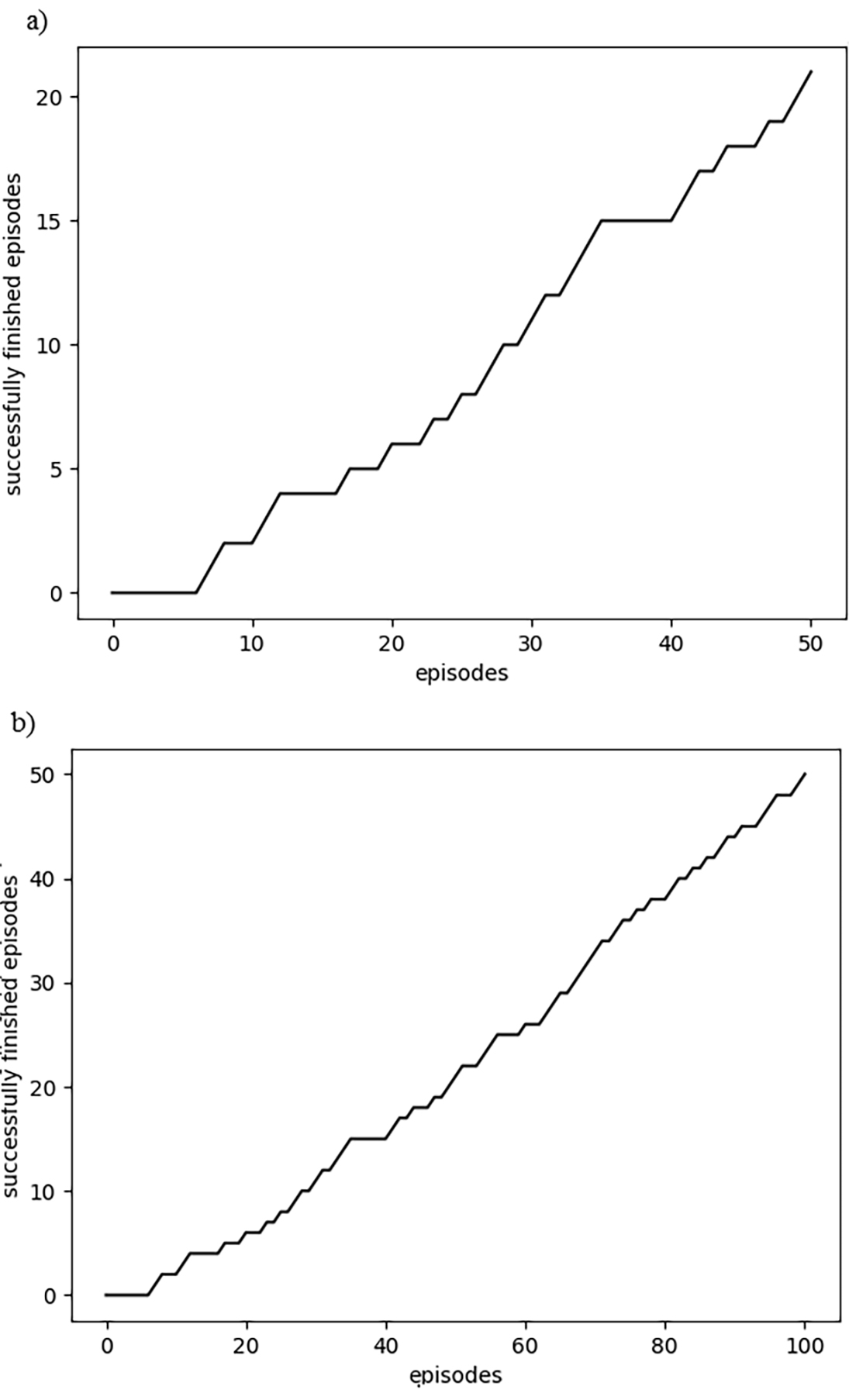
The learning progress of the different RL algorithms is shown in Fig. 9 and Table 1. The running time of different algorithms was not compared. However, the usage of the neural network does not dramatically increase the calculation time because of relatively simple calculations (states as input in a Deep neural network and possible action as output).
In Fig. 9, we see some oscillations during the initial episodes. Then the learning progress stabilizes to the even monotonical growth. Table 1 gives exact estimates of agent success in reaching the destination point. Deep SARSA looks the best starting from the 250th episode.
The efficiency of the proposed model is demonstrated through a real-life collision between two vessels and how to apply the proposed method to avoid collision between vessels. The proposed model could be applied to one vessel or both vessels.
Agent, based on the Deep SARSA algorithm, learning progress.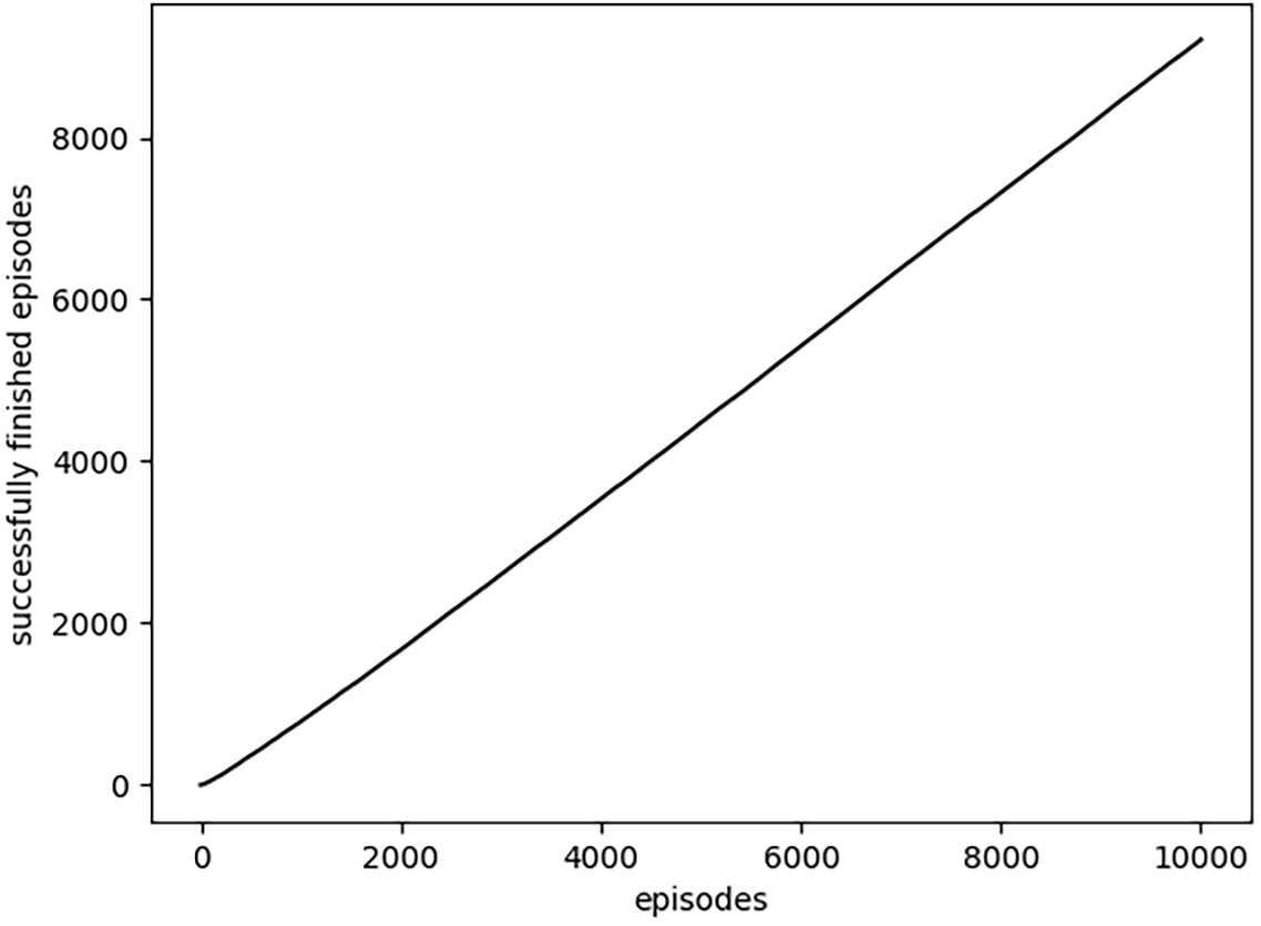
Learning progress of the different simulations carried out with RL algorithms.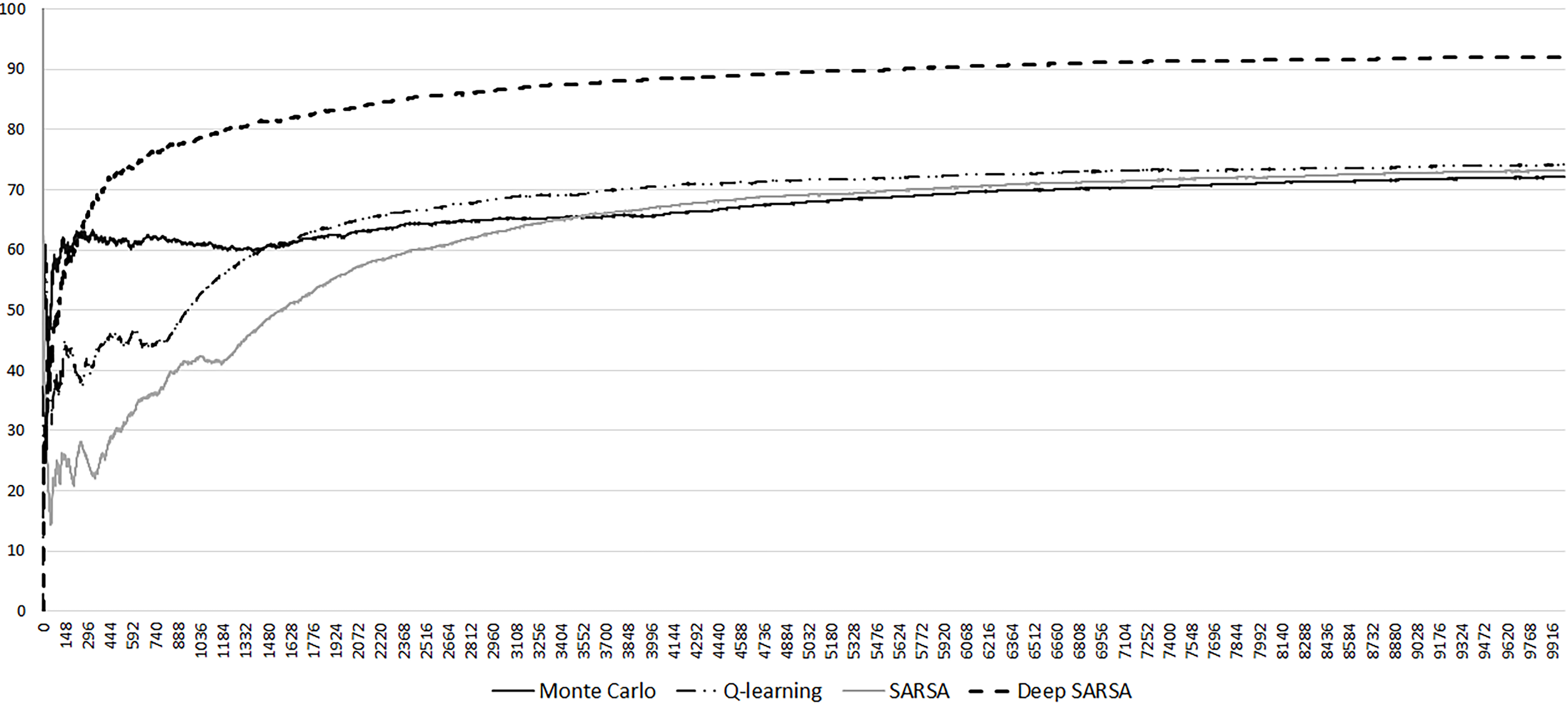
Vessels path and points every 1 minute 30 minutes before the collision.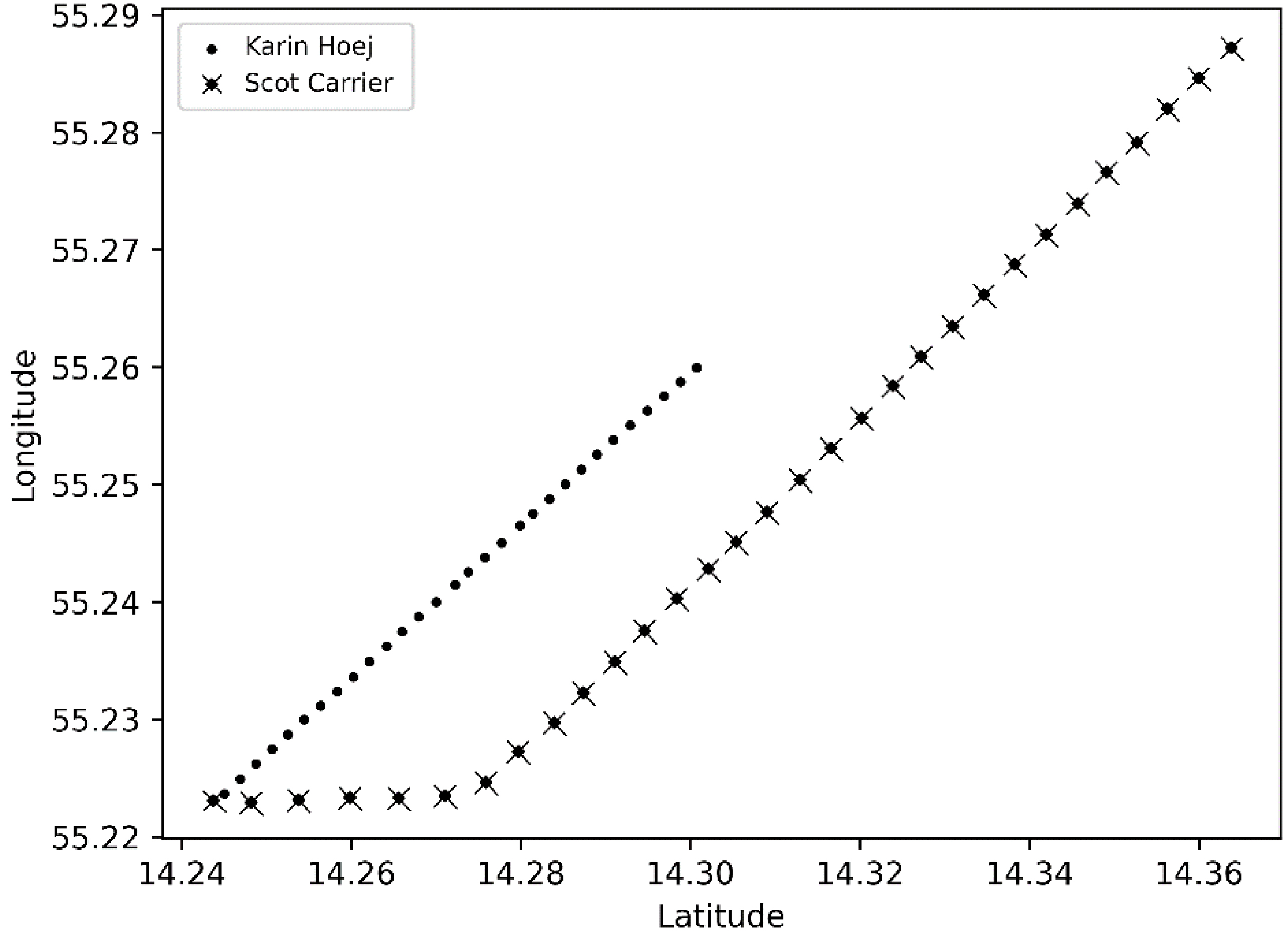
Vessels route and points every 3 minutes 30 minutes before the collision.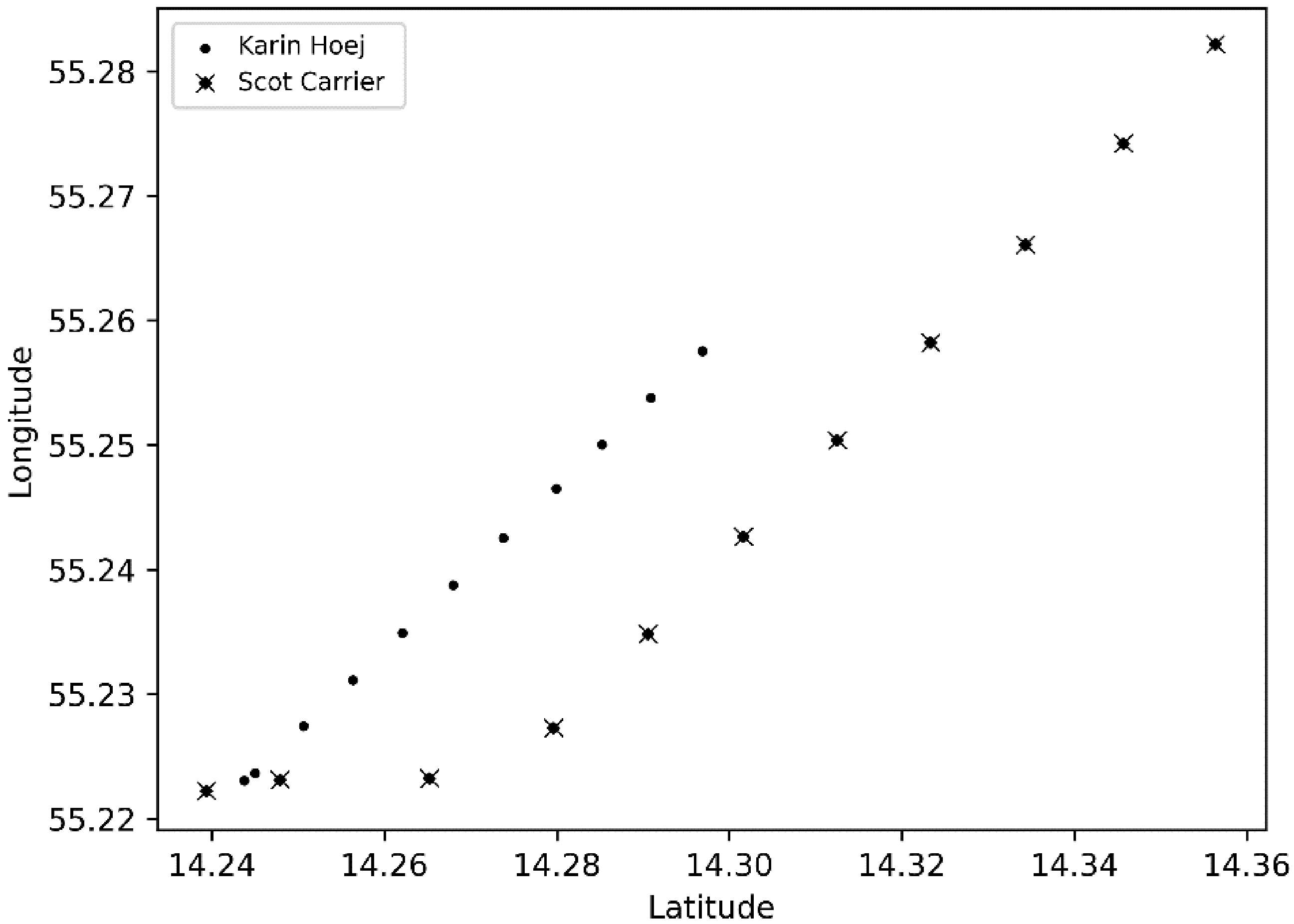
The British cargo vessel Scot Carrier and Danish cargo vessel Karin Hoej collided in the Baltic sea on 13 December 2021. The Karin Hoej capsized, one crew member was found dead, and one person was missing. The main reasons for this collision are gross sea drunkenness and gross negligence in maritime traffic.
Manuvering situation.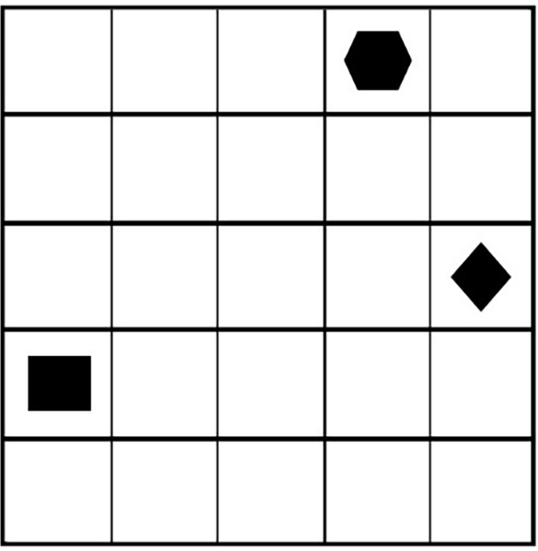
Vessels path and points every 1 minute 9 minutes before the collision.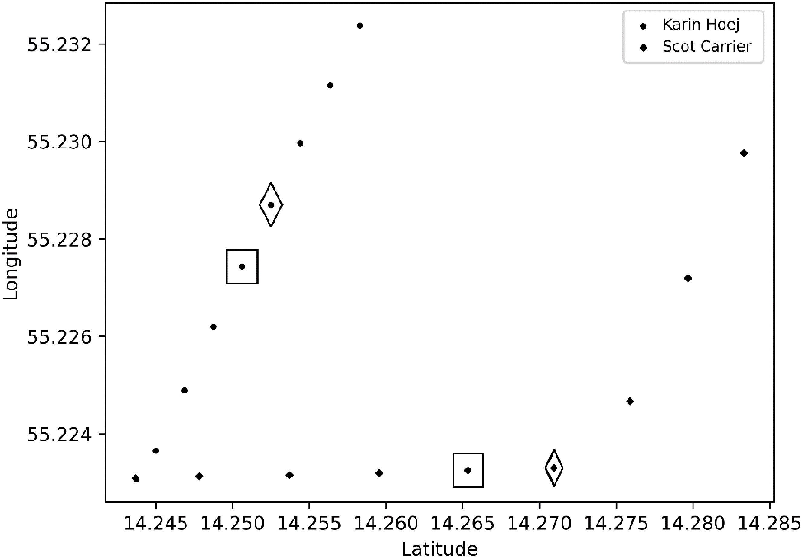
Initial maneuvering situation.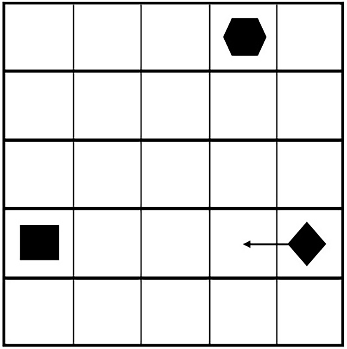
Maneuvering situation.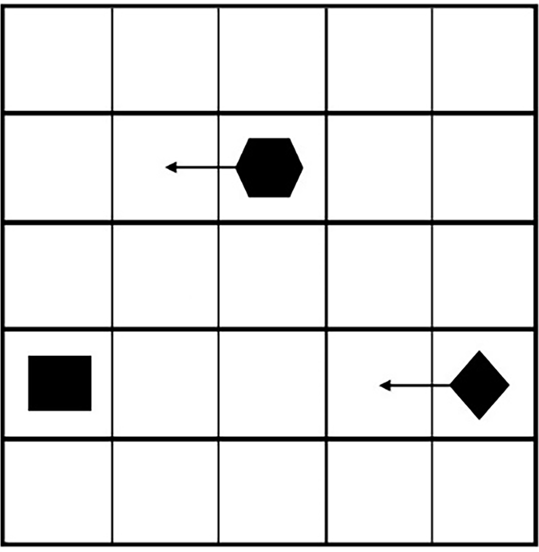
The route of both vessels is shown in Fig. 10. It displays the 30 minutes route before the collision; every point step means every minute of the route. In Fig. 11, every point step means 3 minutes of the route. The Karin Hoej speed was about 7 knots, and the Scot Carrier speed was about 14 knots at the time of the collision. The Scot Carrier tried to bypass Karin Hoej at a safe distance. However, Scot Carrier changed the course to the east, and it caused the collision with Karin Hoej.
In this case, it is important to mention the applied time scale. The main principle of the time scale is the division of the whole maneuvering situation into time steps (time scale) of 1, 3, or 6 minutes. This division comes from the basic sea navigation rules applied in distance and speed calculations. Likewise, such rules are also applied to Radar calculations (speed, distance, etc.).
The usage of the time scale allows the application of the proposed model at different geographical positions. The model is adapted to the relative positions of bend over vessels. Such assumptions allow the application of our model in any geographical position or location. However, it is important to evaluate the relative positions between vessels in a particular maneuvering situation.
Therefore, the proposed model is applied by converting the real geographical positions to a relative. In this example, the square environment is divided into subsquares where the vessel spends 1 min. However, the same procedure could be applied for 3 min or 6 min time step. This division depends mainly on the situation being assessed, i.e. the distance between vessels. Such a method allows us to start assessing the situation in advance.
The difference between real and predicted calculations could be used as an indicator (alarm) of an abnormal maneuvering situation. Moreover, the proposed model could suggest a safe route to avoid a collision or ambiguous maneuvering. The example of the step view is shown in Fig. 11.
Another critical requirement is the point of destination. This point could be obtained by the same distance/time rule – by calculating steps with the time scale of 1, 3, or 6 minutes. In our case, the point of the destination is the 5th point (step) of a further point from the current vessel position of the planned route. As described in the proposed model, each step means a new environment for prediction with current navigational data. At every step (episode), the vessel, as an agent, must avoid collision with an obstacle and recalculate the direction to the position of the destination.
In this example, we applied the Scot Carrier speed for environment calculations with 1 minutes step. Therefore, the square environment correspondent to about 4.6 km
The vessels proceed on a parallel course at a safe distance. There is no danger in such a situation. However, 5 minutes before the collision the Scot Carrier changed course to the Karin Hoej as shown in Fig. 13.
Such maneuvering drastically changed the whole situation. Both vessels started approaching each other. Such a situation is very dangerous in any way. However, nobody on both vessels noticed it. No decision was made in time and a collision occurred.
After the Scot Carrier changed course (the point is marked as rhombus, Fig. 13) navigators of both vessel had to watch closely the situation because such a course clearly led to a collision. At the point marked with a square in Fig. 13, we should apply the proposed model (trained and saved Deep SARSA model). The proposed model analyses the maneuvering situation as shown in Fig. 14.
Figure 14 indicates the possible collision because the vessel could reach the suggested point of destination at the same time. The proposed model could suggest turning right much earlier. It allows evading collision. Firstly, the trained model was applied to the position of Karin Hoej (marked with a hexagon). The recommendation for the Karin Hoey course is shown in Fig. 15.
Secondly, the proposed model was applied for Scot Carrier action (its route is denoted by black squares in Fig. 16). In this case, the trained model proposed the solution for the Scot Carrier as shown in Fig. 16.
Such a real example demonstrates the adaptability of the proposed method for relative comparison of maneuvering situations.
Both suggested vessel courses are shown in Fig. 17. The arrows show the suggested new directions of the analyzed vessels. The course change was suggested 4 minutes before the collision.
Maneuvering situation.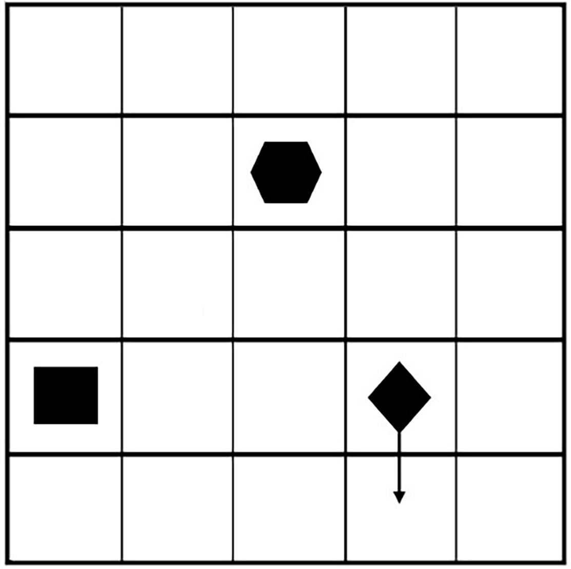
The suggested vessel courses.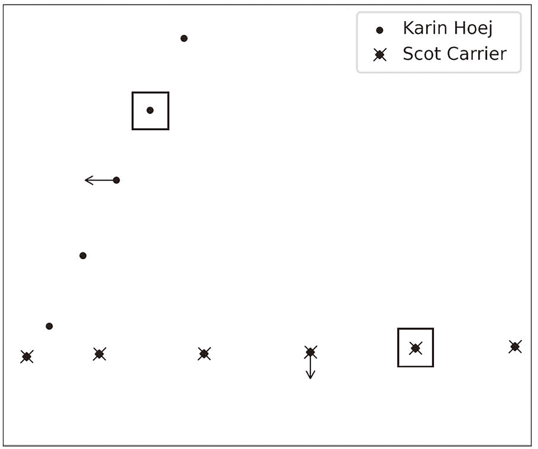
The suggested Karin Hoej course allows to avoid collision and after some time should change course to a planned waypoint. However, the suggested Scot Carrier course is not best in this situation because this suggestion staves off the resolve of such situation. Ideally, the Scot Carrier should change course to the north direction (must go to the top of the image). Nevertheless, both suggested courses could be used as an alarm indicator of an abnormal situation – if there is a difference between the planned route and the proposed one the navigator must evaluate the situation and make the right decision.
In this paper, we have examined RL algorithms to evaluate and find the most appropriate one to ensure safe maneuvering in maritime traffic. It is a crucial real-life problem. The experiments disclose the potential of the Deep SARSA algorithm to solve this problem. This work is a proof-of-concept study, and much more research is needed. Nevertheless, it allows us to identify key trends. Deep SARSA achieves the best precision (92.08%) as compared to Q-learning, SARSA, or Monte Carlo algorithms. This is mainly achieved by applying neural networks to help overcome the learning limits of Q-learning, SARSA, and Monte Carlo. However, the algorithms have been tested in a simplified environment that is not as complex as the real maritime navigation traffic. Due to learning limitations, the RL algorithm cannot operate over a large environment area. Moreover, in maritime traffic, the decision on the further action is stretched in time. RL algorithms tries to find a decision at each step, despite on necessity of the action. Therefore, the best approach to apply the proposed method is to activate the RL algorithm when it is necessary, i.e. when maneuvering starts or a dangerous situation occurs. The efficiency of the proposed model is demonstrated through a real-life collision between two vessels and how it could have been avoided by applying the proposed method.
To conclude, RL algorithms can learn to perform an action or make a decision in a particular situation. This is especially useful for vessel maneuvering in a real environment and for autonomous vessel navigation. The RL algorithm can be applied to help in avoiding human errors by offering a decision in a particular marine maneuvering situation. Nevertheless, significant learning progress must be achieved by designing more robust RL algorithms to discover an optimal strategy.
In future research, we will investigate the application of RL algorithms to control and navigate the vessel in real marine traffic. The application would be used as a recommendation to the navigator or for autonomous navigation. An interesting idea lies in the integration of multi-criteria decision making (see e.g. [60, 61]) with the navigator’s knowledge and experience in the reinforcement learning process. In addition, more complex marine traffic data will be taken into consideration to improve the optimal navigation strategy for real-world applications.