
Abstract
In this paper, a novel Artificial Bee Colony algorithm is proposed to solve a variant of the Job Shop Scheduling Problem where only an interval of possible processing times is known for each operation. The solving method incorporates a diversification strategy based on the seasonal behaviour of bees. That is, the bees tend to explore more at the beginning of the search (spring) and be more conservative towards the end (summer to winter). This new strategy helps the algorithm avoid premature convergence, which appeared to be an issue in previous papers tackling the same problem. A thorough parametric analysis is conducted and a comparison of different seasonal models is performed on a set of benchmark instances from the literature. The results illustrate the benefit of using the new strategy, improving the performance of previous ABC-based methods for the same problem. An additional study is conducted to assess the robustness of the solutions obtained under different ranking operators, together with a sensitivity analysis to compare the effect that different levels of uncertainty have on the solutions’ robustness.
Introduction
The job shop scheduling problem (JSP) in its different variants is considered one of the most relevant problems in scheduling, in part because it is used to model many practical engineering and social applications [1]. It consists in organising the execution of a set of jobs on a set of resources under a set of given constraints in an optimal way. In the literature, this most commonly translates into minimising the project’s execution timespan, also known as makespan. Solving this problem improves the efficiency of chain production processes and has a positive impact on costs and environmental sustainability [2].
Real-world applications of JSP can be generally found in industries where customer orders may differ and have their own parameters; this applies obviously to many manufacturing industries, but also to service industries. For instance, a very common application is semiconductor manufacturing; this includes wafer fabrication, where layers of metal and wafer material are built up in patterns on wafers of silicon or gallium arsenide to produce the circuitry and where each layer requires a number of operations. Another classical example of a job shop is a hospital, where patients can be seen as jobs, so each patient has to follow a given route and has to be treated at a number of different stations while going through the system [3]. A railway scheduling problem can also be modelled as a job shop by dividing the railway network into segments, so each job corresponds to a train trip and operations in a job correspond to the track segments on the train route [4]. Steel mills also have workshops that function as job shops; they produce heavy-duty parts which are processed in different machines, including cutting machines, shaper machines, grinding machines, milling machines, lathes and special turning machines, drilling/boring machines, polishing machines, and painting and drying machines [5]. Another example can be found in the apparel industry, where the job shop is used to model both a progressive bundle system and a unit production system [6]. A wide list of applications of the job shop scheduling in its multiple variants can be found in the survey from [1]. Additionally, real-life applications of the flexible variant of the job shop are reviewed in [7].
To increase its applicability, we must take into account that in real-world situations the available information is often imprecise. Interval uncertainty arises as soon as information is incomplete, and contrary to the case of stochastic and fuzzy scheduling, it does not assume any further knowledge [8, 9]. Moreover, intervals are a natural model whenever decision-makers prefer to provide only a minimal and a maximal duration, and obtain interval results that can be easily understood. Under such circumstances, interval scheduling allows to concentrate on relevant scheduling decisions and to produce robust solutions. Intervals can also be provided if there is some uncertainty about numerical data, as done, for instance, in [10].
Solving scheduling problems with interval uncertainty can also contribute to the active field of fuzzy scheduling [11]. Here, it is common to use fuzzy intervals to represent both uncertainty and preference in parameters, such as ill-known processing times and flexible due dates [12]. Fuzzy intervals are fuzzy sets in the real line whose level-cuts are intervals. Since fuzzy arithmetic is defined via the extension principle for fuzzy sets, operations between fuzzy intervals extend the usual interval analysis into membership functions [13, 14]. Hence, solving a scheduling problem where pure intervals are used to represent ill-known durations provides a first step towards solving problems in the framework of fuzzy scheduling.
Additionally, intervals are inherent to interval-valued fuzzy sets, where the membership degree of an element of the set corresponds to a value in a considered membership interval [15]. Interval-valued fuzzy sets provide an alternative model for ill-known processing times where decision makers find it tough to quantify their judgement about the membership of a possible duration value as a number in the interval
Contributions to scheduling with interval uncertainty are not abundant in the literature. A recent review of publications where intervals are used to model either setup or processing times (or both) in different scheduling problems can be found in [9]. For the job shop, a genetic algorithm is proposed in [18] to minimize the total tardiness when both durations and due dates are intervals. In [19] a different genetic algorithm is applied to the same problem and [20] includes a study of the influence of using different interval ranking methods on the robustness of the resulting schedules. In [21], a hybrid between particle swarm optimisation and a genetic algorithm is used to solve a flexible JSP with interval durations within a more complex integrated planning and scheduling problem. Finally, the JSP minimising makespan with interval durations is tackled using a population-based neighbourhood search in [22], a genetic algorithm in [23] and, more recently, an artificial bee colony method in [24], with the latter achieving the results that constitute the current state of the art and serve as basis for this paper.
The above methods for solving scheduling problems with interval uncertainty belong to the nature-inspired computing paradigm. Indeed, nature-inspired methods have proved very successful in solving complex optimisation [25]. Evolutionary algorithms, inspired in biological evolution, have been widely used for solving complex optimisation problems, many of them with engineering applications [26]. Another well-known group of bio-inspired algorithms are swarm intelligence methods, mimicking the collective behaviour of decentralised, self-organized systems in nature, such as flocks of birds or ant colonies [27]. Together with biology-based algorithms, we find methods inspired in physics [28]. Perhaps the best-known is simulated annealing (SA), based on the principle of thermodynamics [29]. Other example of physics-based method is the harmony search algorithm (HSA), which is a music-inspired population-based metaheuristic algorithm [30]. The gravitational search algorithm (GSA) has its roots in gravitational kinematics [31] while the water drop algorithm (WDA), in hydrology and hydrodynamics [32]. Finally, we can also find chemical reaction optimisation, a population-based meta-heuristic algorithm based on the principles of chemistry [33].
Examples abound in the literature where swarm intelligence methods have been proposed to tackle complex optimisation problems. For instance, cat swarm optimisation, inspired by the biological behaviour of domestic cats, performs very well on binary combinatorial optimisation problems such as 0/1 knapsack [34]. Spider monkey optimisation, based on the social behaviour of spider monkeys is successfully applied to the travelling salesman problem [35]. A particle swarm optimisation (PSO) method with multiple swarms helps improving transfer learning methods in [36], while an ensemble of five particle swarm optimisation strategies is applied to designing the structure of echo state networks in [37]. Another PSO-based method with selective search helps to find good solutions to the university course scheduling problem [38].
There is also an extensive record of successful applications of different metaheuristic methods, most of them nature-inspired, to solving complex engineering problems. For instance, modified versions of the ant colony optimisation algorithm have been proposed to solve high-speed railway alignment and vertical alignment within highway geometric design [39, 40]. A hybrid metaheuristic algorithm that combines harmony search, flower pollination, teaching-learning-based optimisation and Jaya algorithm has been used for the optimization process of active tuned mass dampers, used in structures in the reduction of structural responses resulted from earthquakes [41]. A coronavirus optimisation algorithm combined with long short term memory deep learning has served to forecast deformations of a hydropower dam in [42]. The neural dynamic model of Adeli and Park has been successful in optimising large steel structures [43, 44]. More recently, game theory-based strategies have been incorporated to a Jaya algorithm to improve the computation efficiency and effectiveness in design optimization of civil engineering structures [45].
In particular, artificial bee colony (ABC), a swarm intelligence optimisation template inspired in the foraging behaviour of honeybees, has shown very competitive performance on deterministic JSP with makespan minimisation. For instance, [46] proposes an evolutionary computation algorithm based on ABC that includes a state transition rule to construct the schedules. Taking some principles from genetic algorithms, an improved ABC (IABC) is proposed in [47] that uses a mutation operation to explore the search space, thus enhancing the search performance of the algorithm. An effective ABC approach based on updating the population using the information of the best-so-far food source can be found in [48]. More recently, [24] introduces the idea of having an elite set of bees instead of a queen to improve diversification.
In this work, we tackle the JSP with makespan minimisation and intervals modelling uncertain durations. The problem is presented in Section 2. Building upon our former work in [24], where the employed bee phase was modified, in Section 3 we propose to include a new strategy based on the seasonal behaviour of bees. These variants are compared in Section 4, where the most successful one is also compared with the state-of-the-art. In that section, a robustness analysis is conducted to compare different interval ranking methods, together with a sensitivity analysis on the performance of the algorithm over scenarios with different levels of uncertainty.
The job shop problem with interval durations
In the job shop scheduling problem we have several machines or resources
A schedule
Interval uncertainty
Uncertainty in the processing times of tasks is modelled using closed intervals as done, for instance, in [22, 20]. This approach is appropriate when the lack of historical data does not allow to estimate probabilities and only an upper and lower bound of the likely duration can be provided or when there is uncertainty in numerical data [9, 10]. Under these circumstances, the processing time of a task
The interval JSP (IJSP) with makespan minimisation requires two arithmetic operations: addition and maximum. Given two intervals
Also, given the lack of a natural linear order in the set of closed intervals, to determine the schedule with the “minimal” makespan, we need an interval ranking method. We follow [20] and consider the rankings
Given a schedule
For a task
The makespan is given by the completion time of the last task to be processed according to
A mixed integer formulation of the IJSP can be derived by introducing a binary decision variable
Let
s.t.
The first constraints Eqs (6) and (7) ensure that it is not possible for the starting time of each task to take negative values, while constraint Eq. (8) ensures that the starting time
The makespan obtained for the IJSP under uncertainty is an interval
This is the idea underlying the concept of
where
This robustness measure depends on a particular configuration
This provides an estimate of the robustness of the solution
Simulation techniques such as the one proposed to compute the average robustness are not rare in complex optimisation settings. Simulation allows for modelling and artificially reproducing complex systems in a natural way within affordable computational effort [52]. In particular, our proposal is related to the dominant use of simulation in management science and operations research as a means for system analysis, where the intent is to mimic behaviour to understand or improve system performance [53].
The Artificial Bee Colony (ABC) algorithm is a swarm-based metaheuristic search schema based on the foraging behaviour of honey bees which has been successfully applied with different modifications to a variety of optimisation problems [54]. However, when applied in its standard form to the interval job shop with makespan minimisation, it seems to lead to premature convergence, so a modification was introduced in [24] to improve its diversification capabilities and hence avoid this phenomenon. This method, denoted
In the following we build on
Pseudocode of the Elitist Seasonal ABC[0] An IJSP instance A schedule Generate a pool
In standard ABC, a hive of bees exploits a changing set of food sources (representing solutions to the problem) with two leading models of behaviour: recruiting rich food sources (i.e. keeping promising solutions) and abandoning poor ones (i.e. discarding bad solutions). It starts by generating and evaluating an initial pool
In our proposal, each food source fs encodes an IJSP solution using permutations with repetition [55]. The decoding of a food source follows an insertion strategy, consisting in iterating along the permutation and scheduling each task at its earliest feasible insertion position [23]. Thus, the creation of the initial pool of food sources
Employed bee phase
Originally, the employed bees’ search is always guided by the queen’s food source. That is, each bee combines its food source with the best one in the hive to find a new one. However, this strategy may in some occasions cause a lack of diversity and lead to premature convergence [48]. To address this issue, a modification of the original strategy was proposed in [24] so the guiding food source was instead selected from an elite group. Three different ways of defining the elite group were considered and evaluated.
Once an elite solution
Onlooker bee phase with seasonal behaviour
In this phase, onlooker bees with a food source that is not exhausted (i.e. it has not reached the maximum number of improvement trials) search in the neighbourhood of their food source with a probability
However, a behaviour where bees only move to improving food sources is likely to reduce the search ability of onlooker bees by getting them stuck in local optima. The Scout Bee Phase (Section 3.3) is supposed to solve this issue by discarding those food sources that have not improved after a number of attempts, and replacing them by new random ones. Consequently, new diversity is introduced in the population, but it is a diversity which initial quality might not be adequate to make an effective contribution to the resolution of the problem. Therefore, it seems advisable to allow for certain moves to worsen food sources in the onlooker bee phase with the goal of escaping local optima and avoiding premature convergence.
In nature, honeybees already have this mechanism in place. Seasons have an influence on the honeybees’ thermal behaviour, which might be connected with seasonal shifts of temperature regulated by the honeybee colony. When spring comes, new sources of nectar become available. At that moment, the bees increase their activity to explore larger areas and find the best food sources. This is the time when they accumulate nectar in big amounts and reproduce. By summer, when the daylight period is the longest, bees have already located the best food sources and they make use of the longer days for maximum foraging of nectar. In this period, they focus on honey production and prepare for winter. When freezing temperatures arrive in winter, bees cease their activity in wait for the new spring. In an optimisation context, this resembles a dynamic strategy: at the first stages (spring and reproduction) the swarm focuses on exploration, and as time advances the focus shifts towards exploitation (summer) until it reaches a freezing state (winter). This is analogous to simulated annealing, where a temperature parameter allows for more exploration at the beginning and reduces it as the algorithm advances. The inertia in particle swarm optimisation also has a similar effect, enabling more movement in the first stages, and slowing down when the particles converge to promising areas. A similar idea is also found in memetic algorithms, where local search is combined with population-based evolutionary algorithms and applied with certain probability to balance exploration and exploitation [29, 56].
To mimic this behaviour in our algorithm, we take the food source fs of an onlooker bee and a neighbouring one
Scout bee phase
In this last phase, a scout bee is assigned to each food source that has reached the maximum number of improvement trials. Since this food source has not been improved after the given number of attempts, it is discarded and the scout bee is in charge of finding a replacement. To implement this phase, every food source fs having
Seasonal strategies
To model how temperatures change in our seasonal environment, we get inspiration from simulated annealing algorithms, where temperature is also used to lead the system from states of high energy to states of low energy. To simulate that behaviour, these methods start from an initial temperature
Monotonic strategies
We consider two subcategories of monotonic cooling strategies: multiplicative and additive. In multiplicative strategies, the temperature
Exponential multiplicative cooling (ExpM):
Logarithmic multiplicative cooling (LogM):
Linear multiplicative cooling (LinM):
Quadratic multiplicative cooling (QadM):
In additive strategies, two new values need to be taken into account: the number of cooling cycles NC and the final temperature
Linear additive cooling (LinAd):
Quadratic additive cooling (QadAd):
Trigonometric additive cooling (TrigAd):
Independently of the strategy type, values
Monotonic cooling strategies only take into account the number of iterations of the algorithm. In our case, the temperature of the environment and, with it, the bees behaviour will only depend on the time of the year if a monotonic strategy is used. However, it is reasonable to assume that onlooker bees will be more willing to explore if the food sources around them are poor and they will be more conservative if their neighbourhood is reasonably rich. This would correspond to a non-monotonic adaptive cooling where the temperature
where
To enhance this feature, we propose a new variant of the previous one where
In the experimental analysis, we shall determine which adaptive strategy works better for our problem.
In this section, the different seasonal strategies are evaluated and compared with respect to the best-known solutions in the literature. Also, a study is carried out to determine the advantage (if any) of considering uncertainty during the optimisation process. Different ranking methods for intervals are compared to assess which one yields more robust solutions. Finally, a sensitivity analysis tries to assess the impact of having larger intervals on the solutions.
The experimental analysis is performed on benchmark instances from the literature. Two sets of benchmark instances for IJSP have been proposed in the past: 17 instances in [22] and 12 instances in [23]. The first set of instances is an extension to the IJSP of the well-known crisp instances ORB1 to ORB5 (size
All experiments are done using a C
Parameter analysis
Range of parameter values for each seasonal strategy.
Range of parameter values for each seasonal strategy.
Best parameter setup for variants of ESABC with different seasonality strategies
Average
A preliminary parametric study is conducted to find the best parameter configuration for ESABC. To compare the behaviour of the seven proposed monotonic seasonal strategies, we consider seven different variants of ESABC, namely
Employed bee phase operator: GOX, JOX, PPX Employed bee phase probability: 0.5, 0.75, 1.0 Onlooker bee phase operator: Insertion, Inversion, Swap Onlooker bee probability: 0.5, 0.75, 1.0 Max. number of tries: 10, 15, 20 Size of the elite: 40, 50, 60
In addition, every seasonal strategy has its own specific parameters that need to be tuned: the cooling constant
Finally, the adaptive strategies from Section 3.4.2 are also tested on each variant of ESABC. Table 2 reports the best parameter values for each variant of ESABC. Each row corresponds to one parameter and each column, to one variant of the algorithm. The values in the sixth row, corresponding to the adaptive strategy, are Standard if Eq. (27) is used, Quadratic, if Eq. (28) is used, or Disabled, if no adaptive strategy is used. It would seem that the Quadratic adaptive strategy proposed in this work as a variant of the one in [59] finds better results when combined with the different multiplicative monotonic cooling variants, appearing to be the best option for all of them.
Comparison between GA,
Best solution found by 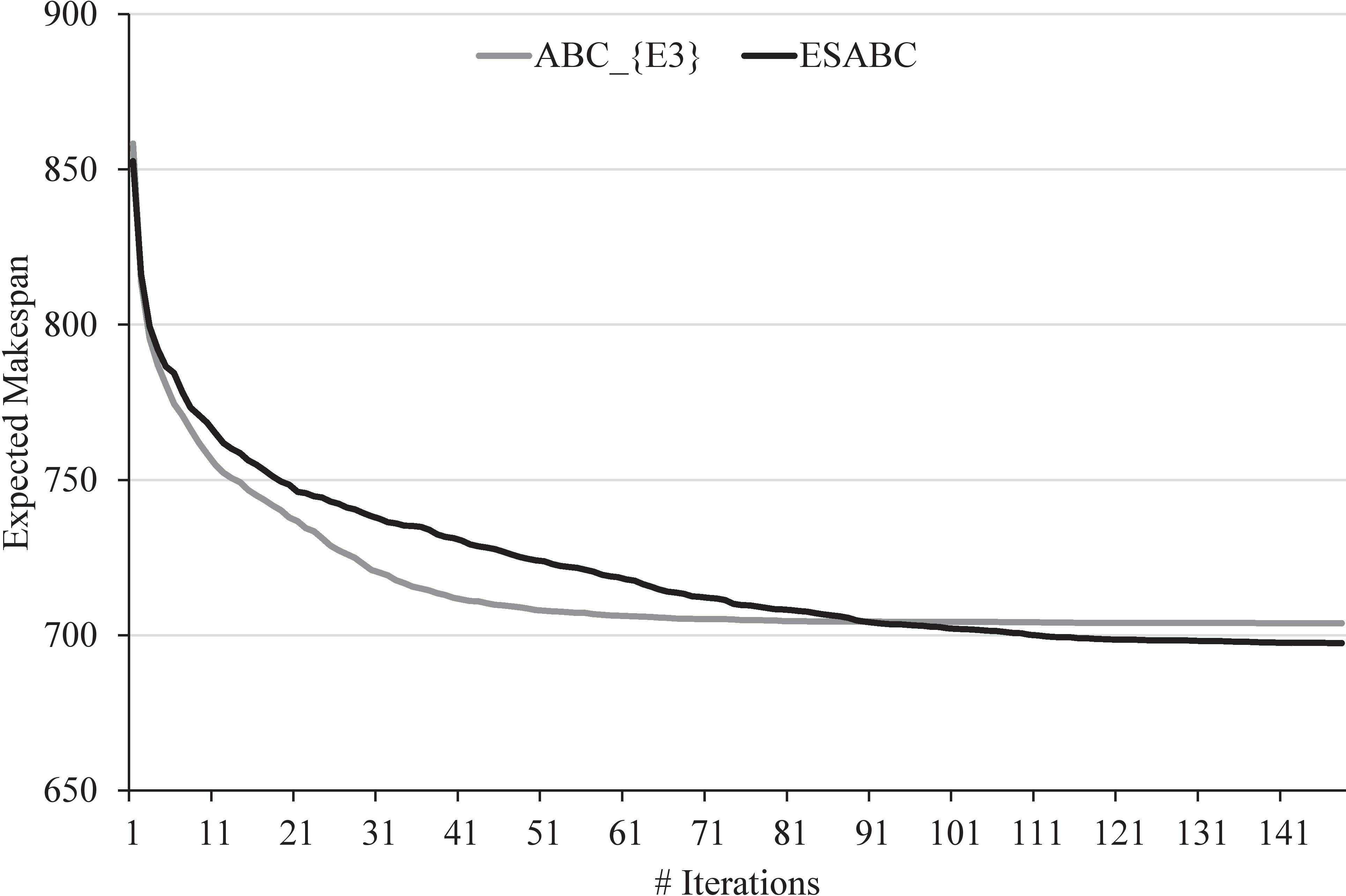
The results obtained with the best setup of each variant are detailed in Table 3. Each row corresponds to one of the instances; the first column contains the name of the instance and the remaining seven columns correspond to the results obtained by ESABC using the different seasonal strategies presented in Section 3.4, so for each seasonal strategy se, the heading of the column
Table 4 reports the comparison of our method with the GA and
Best parameter setup for ESABC using different interval ranking methods
Best parameter setup for ESABC using different interval ranking methods
Average
The comparison is made in terms of Relative Errors (RE) with respect to the best-known lower bound of the problem, shown in the second column of the table. For the sake of clarity, Table 4 shows these errors as percentages. Columns Best and Avg. show the best and average relative errors obtained in 30 runs of each method w.r.t. the given lower bound. Values in brackets represent the standard deviation (SD). Finally, the column Time contains the average runtime of each algorithm. Best average values of each instance are in bold. In terms of the best found values,
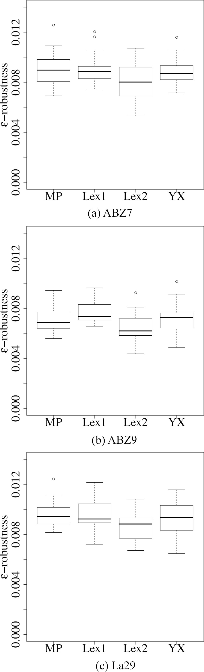
After comparing the different versions of ESABC among themselves and with a state-of-the-art method, we study the effect of using different ranking methods for intervals during the optimisation process. For this study, we focus on ESABC and create four variants of it using the four rankings introduced in Section 2.1. A crisp version of ESABC,
To establish a comparison between all variants, we must take into account that comparisons between intervals depend on the chosen ranking. Since we are comparing the different rankings themselves, choosing a specific one as basis for comparison would be unfair and favour the ESABC variant that used that ranking during the optimisation process. To avoid this problem, the
It is clear that the solutions to the associated deterministic problem are considerably less robust than the solutions obtained incorporating the knowledge about interval uncertainty to the search. In comparison with
Average
To understand why
In that setting, we use the
The average
1000 deterministic realisations of the best solutions obtained by 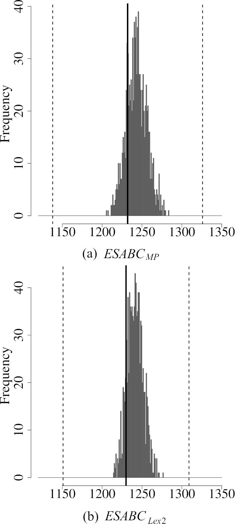
Histograms of 
Histograms of 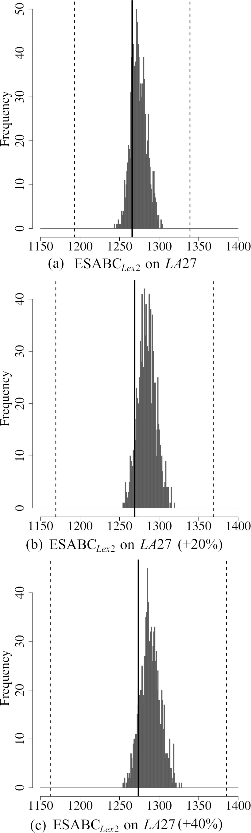
After comparing the algorithm using the instances previously defined in the literature for IJSP, we carry out a new set of experiments on a new set of instances of varied sizes. Our goal is to check the performance of the variant
Employed operator: GOX with probability Onlooker operator: Swap with probability Max. tries: 20 Elite size: 60
Average
Average relative error obtained by 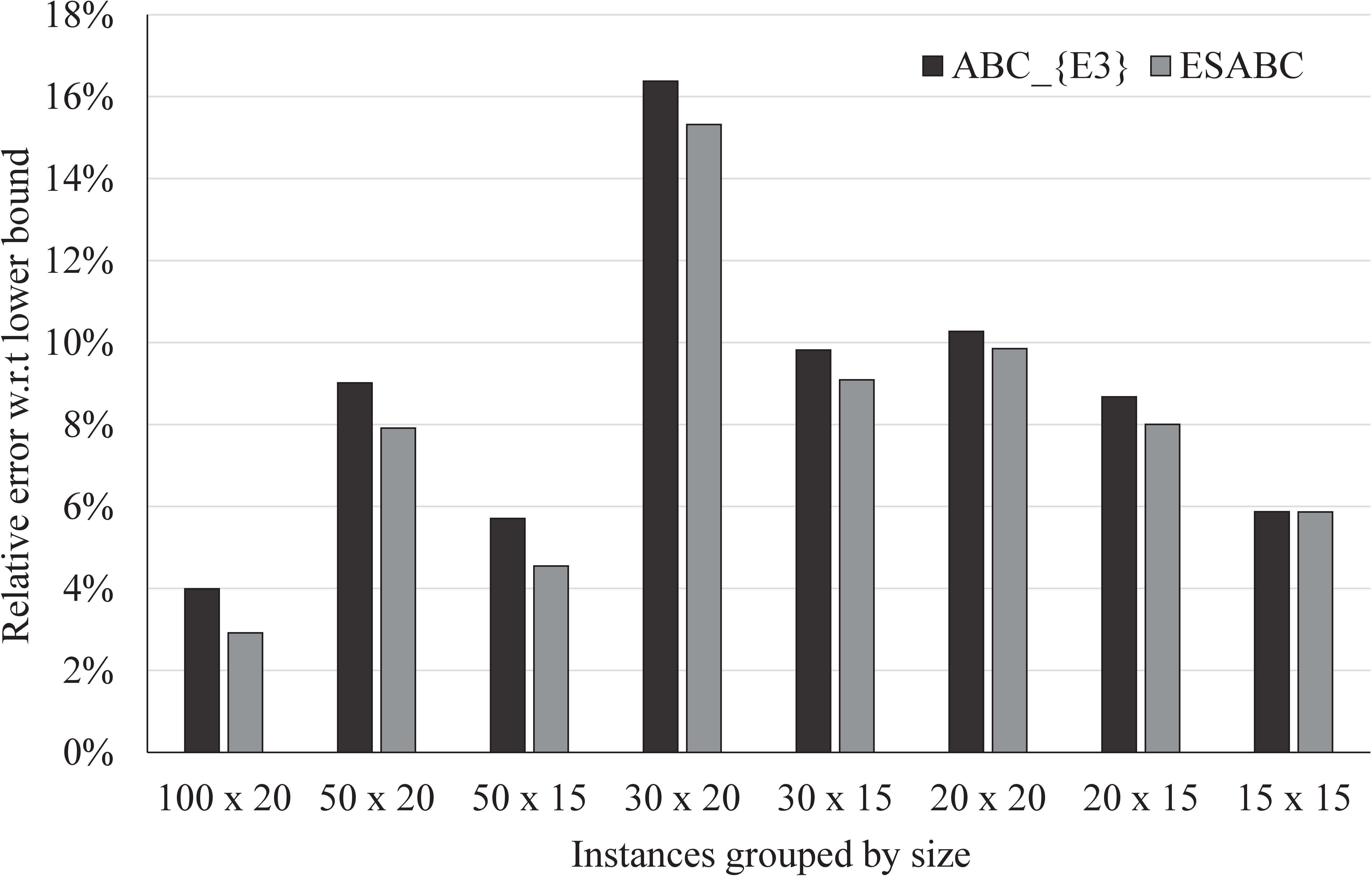
For the parameters that are specific for
Adaptive cooling: Quadratic
As with the previous set of instances, the best results are obtained with the quadratic adaptive cooling scheme. Detailed results on all 80 instances obtained after the parameter tuning can be found in the Appendix. There, Tables 9 and 10 report the best and average
In this work we have confronted the IJSP, a version of the JSP that uses intervals to model the uncertainty on task durations often appearing in real-world problems, with the goal of minimising the makespan. In [24] we used an ABC approach as solving method, adapting the general scheme to our problem, and we tackled the problem of lack of diversity in the swarm by proposing a new ABC variant,
An experimental analysis has shown the potential of the seven variants of seasonal behaviour combined with
In the future, the novel search strategy of ESABC could be applied to combinatorial optimisation problems other than the IJSP. This could be achieved by changing the problem-specific components of the algorithm, that is, the coding of solutions as food sources and their decoding to evaluate the nectar amount, as well as the operators for food-source combination in the employed bee phase and for finding neighbouring food sources in the onlooker bee phase. The general search schema, including the seasonal strategy would remain unchanged.
Also, now that greater diversity is achieved with the seasonal strategy in the search, it would be possible to hybridise the population-based ABC with local search without risking premature convergence to local optima. In this way, the hybrid method could benefit from the synergies between global and local search, as is the case with memetic algorithms, to obtain solutions with higher quality [56].
Finally, it would be interesting to study the effect on the robustness of the solutions obtained with different ranking methods if the Monte-Carlo simulations where obtained using non-symmetric distributions, simulating more extreme scenarios where shorter or larger processing times than expected are more likely to occur.
Footnotes
Acknowledgments
Supported by the Spanish Government under research grant PID2019-106263RB-I00 and by the Asturias Government under research grant Severo Ochoa.
Appendix A. Additional experimental results
Best and average
ESABC
Size
Instance
LB
Best
Avg. (SD)
Time
Best
Avg. (SD)
Time
15
TA1
1231
1289.00
3.7
1286.50
1320.52 (12.91)
5.4
TA2
1244
1277.00
3.9
1284.50
1304.58 (8.99)
5.2
TA3
1218
1262.50
1286.58 (12.40)
4.4
1263.50
5.7
TA4
1175
1226.50
1257.17 (17.39)
4.0
1235.50
5.9
TA5
1224
1263.00
1283.80 (12.82)
3.5
1254.50
5.0
TA6
1238
1280.00
1307.40 (13.05)
4.2
1267.00
5.5
TA7
1227
1261.50
1286.60 (13.08)
3.6
1258.50
5.3
TA8
1217
1248.00
3.9
1241.00
1286.10 (20.72)
5.2
TA9
1274
1331.00
4.1
1343.50
1379.18 (20.15)
5.7
TA10
1241
1280.00
3.8
1287.00
1320.95 (16.13)
5.3
20
TA11
1357
1442.00
1484.13 (16.66)
6.6
1448.50
9.7
TA12
1367
1428.00
1448.93 (10.93)
5.8
1407.00
8.5
TA13
1342
1426.00
7.1
1438.50
1466.07 (15.34)
9.8
TA14
1345
1395.50
1412.52 (15.06)
6.3
1378.50
8.6
TA15
1339
1418.50
1453.27 (17.80)
6.3
1400.50
9.6
TA16
1360
1455.50
6.3
1453.00
1485.33 (28.44)
8.6
TA17
1462
1546.00
1589.52 (20.08)
6.1
1525.00
8.0
TA18
1377
1506.50
1539.35 (14.83)
6.6
1506.00
9.6
TA19
1332
1445.50
1483.32 (18.01)
5.7
1438.00
8.9
TA20
1348
1415.00
1457.00 (18.98)
6.2
1419.00
10.2
20
TA21
1642
1749.00
1774.48 (15.46)
6.9
1731.00
11.2
TA22
1561
1696.00
1725.35 (17.30)
8.1
1689.50
11.8
TA23
1518
1670.00
1693.55 (12.78)
8.0
1662.00
11.8
TA24
1644
1728.50
1766.83 (20.59)
7.8
1731.00
11.0
TA25
1558
1702.50
7.8
1683.50
1732.78 (29.44)
11.2
TA26
1591
1758.00
1798.65 (18.78)
8.4
1750.00
11.7
TA27
1652
1793.50
1824.07 (19.29)
8.3
1775.00
11.6
TA28
1603
1706.50
1734.60 (17.04)
7.5
1703.00
10.9
TA29
1583
1709.50
1744.63 (18.38)
7.6
1704.00
12.0
TA30
1528
1677.00
1714.68 (21.00)
7.7
1681.00
10.6
30
TA31
1764
1870.00
1918.87 (21.63)
12.5
1864.50
18.7
TA32
1774
1963.50
2005.80 (20.28)
13.4
1943.00
19.8
TA33
1788
1956.00
1997.40 (20.46)
13.3
1949.50
18.8
TA34
1828
1978.50
2004.02 (16.49)
12.2
1961.00
17.3
TA35
2007
2036.50
11.7
2039.00
2085.75 (22.44)
13.0
TA36
1819
1963.50
1994.12 (15.63)
12.7
1932.50
18.2
TA37
1771
1915.50
1942.83 (17.27)
12.7
1896.00
16.4
TA38
1673
1815.50
1851.15 (18.12)
12.1
1795.00
18.9
TA39
1795
1905.00
1944.97 (19.65)
13.2
1893.00
18.0
TA40
1651
1835.50
1872.52 (17.79)
13.1
1836.00
17.8
Best and average
ESABC
Size
Instance
LB
Best
Avg. (SD)
Time
Best
Avg. (SD)
Time
30
TA41
1906
2241.00
2297.70 (25.10)
16.1
2217.50
22.4
TA42
1884
2150.50
2212.85 (23.41)
15.3
2156.50
20.8
TA43
1809
2099.50
2136.97 (20.58)
16.5
2059.50
24.2
TA44
1948
2179.50
2228.73 (26.44)
16.8
2152.00
25.9
TA45
1997
2136.50
2185.62 (23.61)
17.0
2132.00
24.2
TA46
1957
2211.50
2268.27 (29.82)
18.2
2198.00
26.2
TA47
1807
2106.00
2176.27 (30.54)
16.3
2084.00
24.0
TA48
1912
2139.50
2177.72 (20.44)
15.1
2128.00
22.1
TA49
1931
2145.00
2185.63 (24.78)
17.1
2135.00
21.3
TA50
1833
2136.50
2206.25 (29.39)
16.3
2135.50
22.1
50
TA51
2760
2912.00
2958.60 (31.68)
27.3
2863.00
40.6
TA52
2756
2867.00
2919.47 (26.24)
27.5
2835.00
43.2
TA53
2717
2816.50
2863.85 (27.06)
27.5
2793.50
37.9
TA54
2839
2857.00
2922.90 (26.70)
24.3
2848.50
34.3
TA55
2679
2840.00
2905.17 (26.14)
29.3
2836.50
39.2
TA56
2781
2871.50
2921.12 (21.82)
23.7
2864.50
36.9
TA57
2943
2991.00
3049.33 (29.99)
26.9
2979.00
41.1
TA58
2885
2974.00
3027.40 (24.09)
26.7
2941.00
38.4
TA59
2655
2804.50
2854.22 (24.07)
27.8
2780.50
38.9
TA60
2723
2843.50
2888.35 (21.77)
24.7
2822.00
34.9
50
TA61
2868
3062.00
3121.43 (29.76)
33.5
3034.50
49.2
TA62
2869
3139.00
3205.95 (29.12)
33.7
3117.50
44.7
TA63
2755
2965.50
3008.20 (23.92)
30.6
2930.00
45.8
TA64
2702
2889.50
2927.90 (20.47)
33.6
2862.50
47.0
TA65
2725
2954.50
2996.90 (27.91)
33.8
2924.00
47.5
TA66
2845
3038.50
3088.55 (21.51)
32.1
3017.00
42.8
TA67
2825
3008.50
3077.80 (27.33)
34.0
3008.50
45.4
TA68
2784
2969.50
3007.00 (22.07)
32.7
2919.50
46.6
TA69
3071
3227.00
3273.53 (28.63)
29.6
3184.50
45.0
TA70
2995
3247.50
3291.77 (20.81)
30.9
3210.50
42.9
100
TA71
5464
5645.50
5723.65 (44.87)
94.2
5581.50
136.0
TA72
5181
5359.00
5409.03 (30.16)
103.1
5283.50
132.4
TA73
5568
5683.00
5735.93 (41.97)
95.3
5631.50
134.5
TA74
5339
5434.00
5512.33 (54.56)
99.5
5391.00
121.7
TA75
5392
5649.50
5731.18 (33.34)
105.0
5618.00
127.7
TA76
5342
5535.00
5586.72 (35.81)
101.2
5481.50
126.5
TA77
5436
5529.50
5616.35 (65.01)
107.0
5492.50
133.5
TA78
5394
5490.00
5535.08 (29.19)
102.7
5426.00
125.5
TA79
5358
5446.00
5502.72 (33.76)
107.8
5418.50
125.9
TA80
5183
5373.00
5440.45 (35.15)
107.1
5339.00
138.5