Enhancing peak prediction in residential load forecasting with soft dynamic time wrapping loss functions

Abstract

Short-term residential load forecasting plays a crucial role in smart grids, ensuring an optimal match between energy demands and generation. With the inherent volatility of residential load patterns, deep learning has gained attention due to its ability to capture complex nonlinear relationships within hidden layers. However, most existing studies have relied on default loss functions such as mean squared error (MSE) or mean absolute error (MAE) for neural networks. These loss functions, while effective in overall prediction accuracy, lack specialized focus on accurately predicting load peaks. This article presents a comparative analysis of soft-DTW loss function, a smoothed formulation of Dynamic Time Wrapping (DTW), compared to other commonly used loss functions, in order to assess its effectiveness in improving peak prediction accuracy. To evaluate peak performance, we introduce a novel evaluation methodology using confusion matrix and propose new errors for peak position and peak load, tailored specifically for assessing peak performance in short-term load forecasting. Our results demonstrate the superiority of soft-DTW in capturing and predicting load peaks, surpassing other commonly used loss functions. Furthermore, the combination of soft-DTW with other loss functions, such as soft-DTW $+$ MSE, soft-DTW $+$ MAE, and soft-DTW $+$ TDI (Time Distortion Index), also enhances peak prediction. However, the differences between these combined soft-DTW loss functions are not substantial. These findings highlight the significance of utilizing specialized loss functions, like soft-DTW, to improve peak prediction accuracy in short-term load forecasting.

Keywords

Short-term load forecasting loss function dynamic time wrapping soft-DTW deep learning peak prediction

1. Introduction

Load forecasting can be a valuable contribution to power system operation and the decision-making process of unit commitment. The transition from traditional centralized power stations to the decentralized energy system becomes more and more popular, as it allows for more optimal use of renewable energy and provides the possibilities for small energy producers to better connect with end-users. Microgrids, as one of the most effective forms of decentralized energy systems, gather facilities to generate, supply, and store electricity with or without the support of the centralized macrogrid [1]. Despite many advantages of microgrids, a smart control system is highly demanding due to the technical challenges associated with the control system. Smart grid is an intelligent electricity network with the integration of the users’ behaviors and actions to manage the volatility from multiple types of small power producers and small-scale electrical transmission and distribution networks [2]. One of the essential tasks of smart grid is short-term load forecasting with high granularity and precision to match demands and generations. Unlike the national aggregated load forecast, the disaggregated load, especially at the individual level, is hard to predict with rapid fluctuations and different user behaviors, making short-term residential load forecasting at the individual level challenging.

Before the success of artificial intelligence, load forecasting was carried out with physically explicit methods [3]. These models are based on heat and transfer equations to calculate energy consumption with detailed thermo-physical information. This physically explicit method can be described as a white box composed of explicit equations describing measurable variables. The advantage of the physically explicit method is that it does not rely on any historical data to perform load prediction. However, it requires the knowledge of many thermo-physical parameters which are not always easy to access. Therefore, it is challenging and time-consuming when addressing large and complex use cases with the physically explicit method. Another important limitation of such approaches is the complexity of the resulting models when taking into account all involved phenomena. Hence, simplifying assumptions are often chosen in order to obtain a less computationally expensive model, such as simplified user behaviors.

The development of smart electricity meters enables the collection of large datasets, making the data-driven model feasible for load forecasting. Deep neural network as one of the prominent techniques in artificial intelligence, has been proposed for short-term load forecasting within the last two decades [4]. As a data-driven approach, it does not require either thermo-physical information or occupant behaviors, but only historical data compared to the previous physically explicit model. Numerous studies have demonstrated the effectiveness of deep neural networks in short-term load forecasting [5, 6, 7, 8]. And there are different approaches to improve its performance by modifying the architecture of the neural network [9, 10] or adding preprocessing techniques [11, 12]. But only very few studies focus on the analysis of loss functions.

Mean squared error (MSE) has been primarily employed as a loss function for regression to train neural networks for short-term load prediction [13, 14, 15, 16]. Li et al. [17] compared mean absolute percentage error, cross-entropy, and mean absolute error (MAE) for the aggregated load. Dudek [18] added weights into MSE for different training samples. A critical constraint of training with these loss functions is that they measured the cumulative errors along the target time series without specific consideration of load shape. As a result, they may exhibit less capability to accurately predict peak loads, which is crucial for short-term load forecasting. Dynamic time wrapping (DTW) [19] may be a possible solution. It aims to find an optimal alignment between two time series. As it concentrates on the time series similarities, it may add more importance to the load shape of the prediction task in order to strengthen peak load forecasting. Because of its ability to measure the similarities between curves, DTW has been mainly used for clustering algorithms [20], but less for regression because of its non-differentiability for gradient descent optimization. In 2007, soft-DTW [21], a differentiable formulation of DTW, has been proposed to fit better the backpropagation of neural networks. It has demonstrated considerable success in clustering applications [22, 23, 24, 25, 26], while its application and analysis in the field of load prediction have been relatively limited [27]. Besides, the drawback of soft-DTW has been discussed in the literature, Le Guen and Thome [28] demonstrated its incapacity of capturing temporal distortion and proposed incorporating an extra term to the soft-DTW loss function: time distortion index (TDI). This combined loss function has gained attention in the task such as time series imputation task [29] and PM2.5 concentration prediction [30]. However, it is relatively rare discussed in load prediction.

Therefore, the main objective of this article is to conduct a thorough comparative analysis of the soft-DTW loss function in relation to other loss functions, with a specific focus on its peak prediction performance. Many existing studies used peak loads as the inputs and outputs for training [31, 32, 33], it is rare to find evaluations on peak prediction performance when forecasting the entire time series. Thus, we introduce in this article a novel evaluation methodology using confusion matrix and propose new errors for peak position and peak load, tailored specifically for assessing peak performance in short-term load forecasting.

The article is organized into three main parts:

•
Analysis of soft-DTW loss function: In this part, we provide an introduction to soft-DTW and the proposed neural network architecture, followed by a comparison to the result presented in the literature on a benchmark dataset to validate our model. Then three loss functions: soft-DTW, MAE, and MSE were compared on a real dataset from Irish residential buildings to give insights into the improvement of soft-DTW and the limitations of common error metrics.
•
Peak evaluation: In this part, we give the definition of our new error metrics, namely peak position error and peak load error. We then evaluate the previous results using these error metrics and the confusion matrix to demonstrate how the utilization of soft-DTW loss function can enhance the accuracy of peak load forecasting.
•
Combined soft-DTW loss functions: In this part, our focus is on comparing three different combined loss functions, namely soft-DTW $+$ MSE, soft-DTW $+$ MAE, and soft-DTW $+$ TDI. We aim to gain insights into how the incorporation of different loss components, such as MSE, MAE, and TDI, impacts the predictive capabilities of the soft-DTW algorithm.

2. Part I: Analysis of soft-DTW loss function

2.1 soft-DTW

Dynamic Time Wraping was first introduced in 60s [34] and developed for speech recognition [19] and pattern discovery [35] later. It measures the similarity between series considering the deformation of the curves, which is defined as the sum of the values from the cost matrix along this shortest path:

$\displaystyle\textit{DTW}(\hat{\bm{y}},\bm{y})=\min\limits_{\bm{A}\in\mathcal{% A}_{N,M}}\langle\bm{A},\Delta(\hat{\bm{y}},\bm{y})\rangle$ (1)

where $N$ , $M$ denotes the length of compared sequence respectively, $\bm{A}$ is the binary alignment matrix of size $N\times M$ in its set of all alignment $\mathcal{A}_{N,M}$ , $[\Delta(\hat{\bm{y}},\bm{y})]_{i,j}=\delta(\hat{y}_{i},y_{j})$ is the cost matrix of size $N\times M$ pairwise distance between predicted value $\hat{\bm{y}}$ and ground truth $\bm{y}$ . $\langle\cdot,\cdot\rangle$ is the inner product of matrix. In this article, we use Euclidean distance for $\delta$ to calculate the cost matrix.

However, DTW is not differentiable everywhere. Cuturi and Blondel [21] proposed soft-DTW, a differentiable formulation of DTW by smoothing min operator from Eqs (1) and (2.1) with non-negative smoothing parameter $\gamma$ :

$\displaystyle\textit{DTW}_{\gamma}(\hat{y},y)$ (2) $\displaystyle=\left\{\begin{array}[]{ll}-\gamma\log\sum\limits_{A\in\mathcal{A% }_{n,n}}\exp\left(-\frac{\langle A,\Delta(\hat{y},y)\rangle}{\gamma}\right)&% \gamma>0\\ \textit{DTW}(\hat{y},y)&\gamma=0\end{array}\right.$

If $\delta$ is differentiable everywhere as well, then soft-DTW when $\gamma>0$ is differentiable in all of its variables, in our case, $\delta$ is euclidean distance. And the gradient of soft-DTW when $\gamma>0$ is derived from Eq. (2.1):

$\displaystyle\nabla_{\Delta}\textit{DTW}_{\gamma}(\hat{\bm{y}},\bm{y})$ (3) $\displaystyle=\frac{\sum\limits_{\bm{A}\in\mathcal{A}_{N,M}}\exp\left(-\frac{% \langle\bm{A},\Delta(\hat{\bm{y}},\bm{y})\rangle}{\gamma}\right)\bm{A}}{\sum% \limits_{\bm{A}\in\mathcal{A}_{N,M}}\exp\left(-\frac{\langle\bm{A},\Delta(\hat% {\bm{y}},\bm{y})\rangle}{\gamma}\right)}$

2.2 Proposed neural network: Residual LSTM

2.2.1 Residual block with skip connections

Skip connections shown as additional paths between layers reduce the length of gradient flow from output layers to the lower layers, thus easing neural network training [36]. One of the most successful applications of skip connections is ResNet [37], with multiple small residual blocks to train deeper neural networks. Li et al. [38] presented a visualization of the loss surfaces of ResNet with the comparison of skip connections. It indicated that the skip connection smooths the loss landscape of neural networks to make it easier to converge. Because of its effectiveness, many different neural network architectures with skip connections have been designed for load forecasting: Kiprijanovska et al. [39] chose fully-connected layer as the inner structure of residual block while Gong et al. preferred long short-term memory (LSTM) as internal layer [40]. Besides, temporal convolutional networks which have gained attention recently for load forecasting [14, 41] also adopt skip connections to ease the training.

Another reason to choose residual block, which has not been shown in the other references is the explanation of prior knowledge for load forecasting. Because the load profile of day $d+1$ usually does not change much compared to day $d$ , in order to predict the real value of $d+1$ , it is convenient to predict the residual of the day $d+1$ to the day $d$ where the identity shortcut of residual block serves the need.

Figure 1.

Residual LSTM neural network.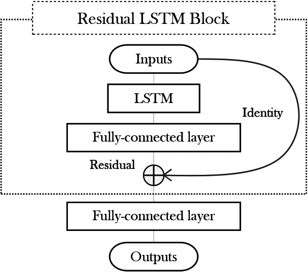

Figure 2.

DBA K-means clustering of first two weeks loads for 929 residential users.

Figure 3.

Flowchart of proposed methodology.

Figure 4.

Residential load predictions with MSE, MAE, soft-DTW loss functions from 2010-11-10 to 2010-11-16.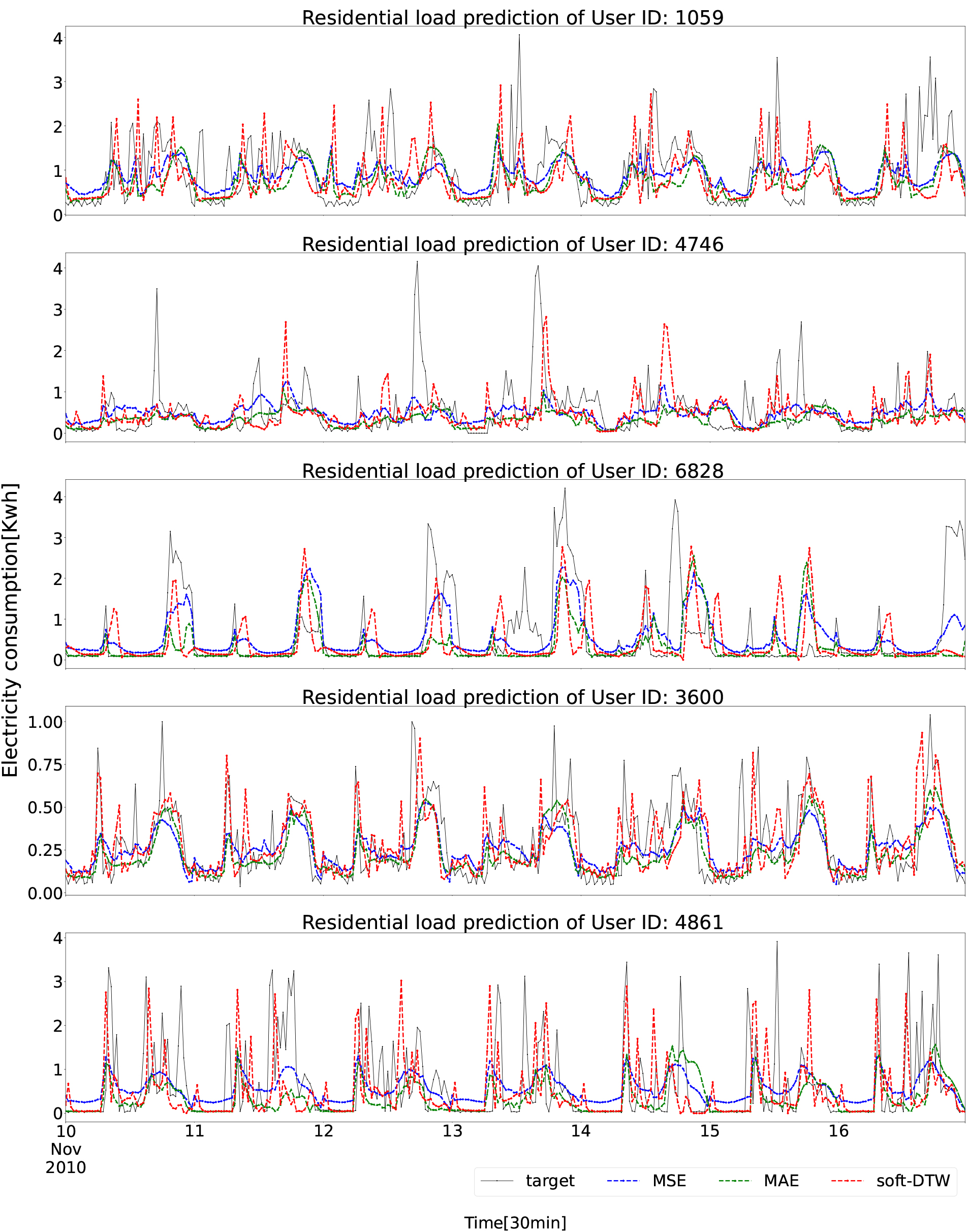

Figure 5.

Daily dynamic time warping error with MSE, MAE, soft-DTW loss functions.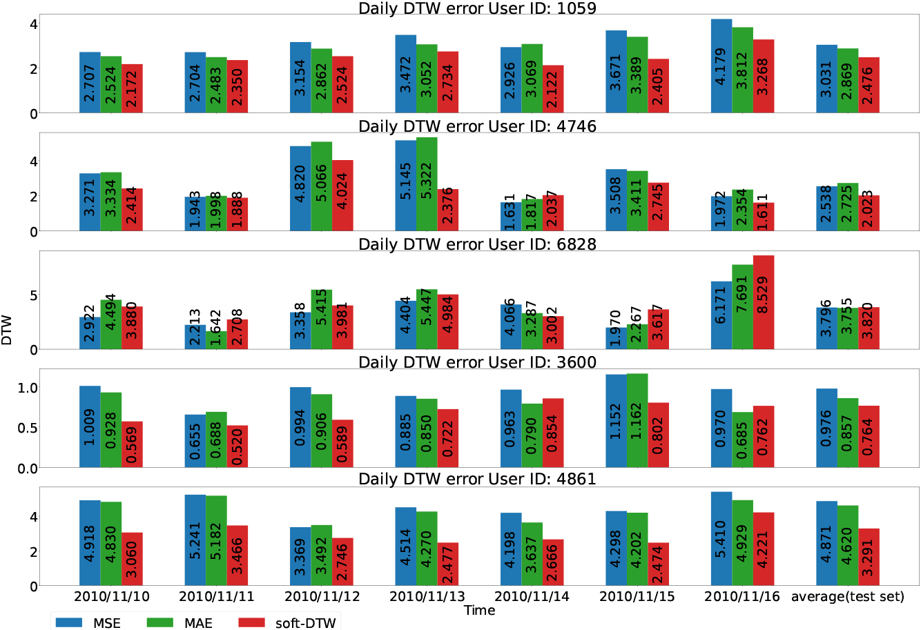

2.2.2 LSTM

Recurrent neural networks (RNN) is one of the most common neural networks for sequence modeling thanks to the feedback connections to share parameters over time. However, due to the vanishing and exploding gradient problem, the variant named gated RNN is more commonly used for long sequences. Short-term load forecasting is not only influenced by the variables at the current time but also the past pattern, for instance, the profile of the last 24 hours, which explains the popularity of two gated RNNs for short-term load forecasting: LSTM and gated recurrent unit (GRU) [12, 42, 43, 44]. Therefore, in this paper, one of the most popular gated RNNs, namely LSTM with residual connection is selected (shown in Fig. 1) for the following comparison. The logic of this residual LSTM block design is to learn the characteristics of residual load with LSTM before addition operation and then add the identity shortcut to form the real load for the next fully-connected layers.

2.2.3 Validation on benchmark dataset

To validate our proposed neural network, we followed the same procedure as Mocanu et al. [45]: Dividing the benchmark dataset, which consists of three years of electricity consumption data from a residential building in France [46], into a training set covering the period from 2007-12-16 to 2009-12-16, and a test set spanning from 2009-12-17 to 2010-11-26; Filling the missing values with the mean values of the corresponding minutes from the other years.

For our Residual LSTM network, we employed 128 neurons with a many-to-many architecture, followed by a two-layer fully-connected neural network with 16 and 1 neurons, respectively. The configuration of the last fully-connected layer is identical to the setting of the fully-connected layer inside the residual LSTM block. We used the batch size of 1000 and the learning rate of 1e-05, with EarlyStopping and the Adam optimizer. The model was implemented and trained using PyTorch.

We evaluated the performance of one-day-ahead prediction for aggregated active power with 15 min resolution as this scenario is commonly encountered in practical applications. To ensure a fair comparison, we utilized the same loss function, mean squared error, as presented in Mocanu et al. [45]. The results are summarized in Table 1, which includes a comparison between our proposed model and other existing approaches, such as artificial neural networks with all fully-connected layers (ANN), support vector machines (SVM), recurrent neural networks (RNN), conditional restricted Boltzmann machines (CRBM), and factored conditional restricted Boltzmann machines (FCRBM), as reported in the reference. Notably, our model Residual LSTM achieves the lowest root mean squared error (RMSE), providing validation for its effectiveness.

Table 1
One-day-ahead prediction with 15 min resolution

	Methods	RMSE
Mocanu et al. [45]	ANN	0.9072
	SVM	1.3446
	RNN	1.0092
	CRBM	1.0305
	FCRBM	0.8995
	Residual LSTM	0.7924

2.3 Comparison of soft-DTW, MSE, MAE loss function on real dataset

Recognizing the limitations of the benchmark data-set, which included data from only one residential building, a richer dataset from the Republic of Ireland [47] was chosen to facilitate a more comprehensive comparison of the loss functions. Additionally, it is worth noting that the division of a dataset into train and test set without a validation set may impact the final result since the test set has been used for tuning the model’s hyperparameters. To address this concern, in this section, we divided the dataset into three subsets: train set for training, validation set for tuning, and test set for final evaluation.

The Irish residential dataset, namely CER, contains 4232 Irish residential consumers with three variables: meter ID, time, and load from 1st July 2009 to 31st December 2010 with a time interval of 30 min. Among 4232 residential users, there are 929 in the controlled group without changeable tariffs and demand side management informational stimuli. It is time-consuming to train all 929 residential users, thus we select 5 representative loads after clustering the first two weeks of 929 residential users into 5 groups with DBA K-means [48] to present the effect of different loss functions. All the loads are standardized before clustering, the result is shown in Fig. 2.

Each cluster group contains 176, 94, 370, 166, 123 users respectively. We randomly select one load as a representative of each cluster group. The user IDs selected are: 4861, 3600, 1059, 6828, 4746. Datasets are split into train sets of the first 70% datasets, validation sets of the next 20% and the last 10% as test datasets for the prediction model. The target datasets to predict are unseen, so the standardization is based on the training set with its mean and standard deviation. The load is standardized during training, but the errors for comparison are recomputed on the original scale. The goal is to predict the next-day profile with an input sequence length of 48. During the training phase, inputs and outputs are batched with a sliding window of 30 min to enlarge the dataset, while the evaluation phase is based on next-day prediction with a sliding window of 1 day. Details are shown in the flowchart (see Fig. 3).

The configuration of the neural network is the same as in the previous section. Batch size $\{300,500,1000\}$ and learning rate $\{10^{-3},10^{-4},10^{-5}\}$ are tested for each case to reach the best result. The smoothing parameter $\gamma$ is set to 0.01. All the trained models are not integrated with the regularizer in order to prevent comparison from its influence.

The prediction results in the test set from 2010-11-10 to 2010-11-16 with MSE, MAE, and soft-DTW loss functions are presented in Fig. 4.

It clearly demonstrates that the soft-DTW loss function outperforms the MSE and MAE loss functions in capturing the majority of the dynamics and peaks for all five residential buildings. This effect is related to the emphasis on the similarity of the curves rather than the cumulated error from the theory of DTW. In other words, models are trained to focus on learning the pattern of the profile with more capability to predict peaks.

To quantitatively analyze this effect, daily DTW prediction error is first compared. Error metrics from 2010-11-10 to 2010-11-16 and average daily DTW error on the test set are shown in Fig. 5.

Based on the results presented in this figure, DTW error roughly presents the peak prediction performance as the soft-DTW loss function has the lowest DTW error in most cases. However, DTW error cannot fully depict this performance. For instance, the residential building with ID: 3600 on 2010-11-16 has a lower DTW error with the MAE loss function. But Fig. 4 shows that soft-DTW loss functions are able to predict the two major peaks while the MAE loss function fails. The reason that soft-DTW has higher DTW error may be due to the two prediction peaks around 18:00 with position error.

To address this problem, a more precise evaluation of errors should be conducted, specifically focusing on peak prediction performance, which includes both peak position errors and peak load errors.

It is important to note that soft-DTW increases its ability of peak prediction but meanwhile sacrifices its cumulated error MSE and MAE. Table 2 reveals that the soft-DTW function exhibits the highest MSE and MAE prediction error on the test set.

Table 2
MSE and MAE on test set for different loss functions

Loss function	buildingID	MSE	MAE
soft-DTW	1059	0.466	0.455
	4746	0.333	0.342
	6828	1.097	0.606
	3600	0.044	0.143
	4861	0.972	0.613
MSE	1059	0.363	0.425
	4746	0.256	0.327
	6828	0.716	0.502
	3600	0.033	0.130
	4861	0.741	0.562
MAE	1059	0.397	0.403
	4746	0.269	0.276
	6828	0.831	0.464
	3600	0.032	0.120
	4861	0.851	0.561

3. Part II: Peak evaluation

In the previous section, we observed an improvement in peak prediction performance through the utilization of soft-DTW. However, the common error metrics such as MSE, MAE, and DTW were unable to adequately capture this improvement. Thus, there is a need for a new measurement specifically designed to assess the peak load performance, which would provide a clearer representation of the observed enhancement.

Figure 6.

Confusion matrix of peak performance on test set.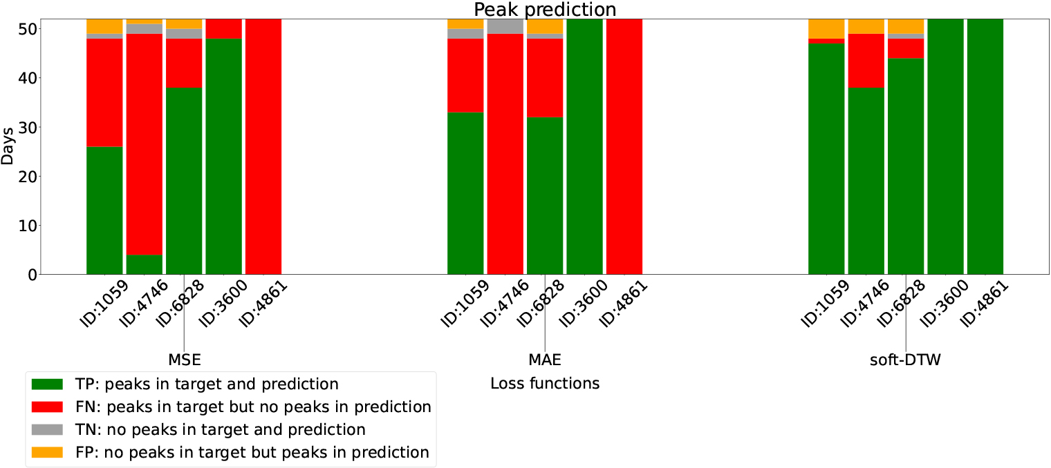

When evaluating peak load prediction, it is common to calculate error metrics such as MSE directly between the real peaks and the forecasted peaks. This approach is frequently applied when both the inputs and outputs are peak loads [31, 32, 33, 49, 50]. However, in our case, where we predict the entire time series, this evaluation method is not applicable as the number of peaks in the prediction may differ from those in the target. Therefore, directly accumulating these errors is not straightforward. In addition, since we predict the entire time series, we introduce another error measurement that is rarely analyzed in the literature: peak position error. Hence, when the number of peaks in the prediction does not match those in the target, two measurements need to be defined:

•

peak load error

•

peak position error

3.1 Peak position error and peak load error

To tackle this problem, the idea is to associate each peak in prediction with its nearest peak in the target, and then calculate the error respectively. Inspired by the DTW algorithm that was presented before, this association can be formulated as the match in the DTW path between the index of peaks, then the DTW path cumulates the distance between these pairs of peaks which represents the peak position error of two curves. We define this error as follows:

$\displaystyle E_{\textit{peak position}}=\textit{DTW}(\hat{\bm{I}},\bm{I})$ (4)

where $\hat{\bm{I}}$ and $\bm{I}$ denote the index of forecasted peaks and target peaks respectively.

Once peaks are matched, similarly we define the peak load error:

$\displaystyle E_{\textit{peak load}}=\langle\bm{A}^{*},\Delta(\hat{\bm{p}},\bm% {p})\rangle$ (5)

where $A^{*}$ denotes the optimal alignement of Eq. (4), $\hat{p}$ and $p$ denote the forecasted peak loads and target loads respectively.

3.2 Confusion matrix

In this article, peaks are defined as all local maxima that are higher than 1/3 of the global maximum. To analyze the model’s ability to predict peaks, four scenarios are defined based on the confusion matrix:

Table 3
Confusion matrix of peak prediction

	Peaks in target	No peaks in target
Peaks in prediction	TP	FP
No peaks in prediction	FN	TN

•

True Positive (TP): model successfully predicts peaks when peaks are presented in the target

•

False Positive (FP): model predicts peaks however there are no peaks in the target (Type Error I)

•

False Negative (FN): model failed to predict peaks when peaks are presented in the target (Type Error II)

•

True Negative (TN): there are no peaks in target and prediction

Table 4

Confusion matrix of peak performance on test set

Days	MSE					MAE					soft-DTW
	1059	4746	6828	3600	4861	1059	4746	6828	3600	4861	1059	4746	6828	3600	4861
TP	26	4	38	48	0	33	0	32	52	0	47	38	44	52	52
FN	22	45	10	0	52	15	49	16	0	52	1	11	4	0	0
TN	1	2	2	0	0	2	3	1	0	0	0	0	1	0	0
FP	3	1	2	0	52	2	0	3	0	52	4	3	3	0	0

Figure 7.

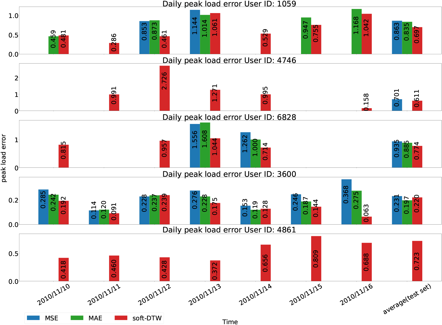
Daily peak load prediction error with MSE, MAE, soft-DTW loss functions.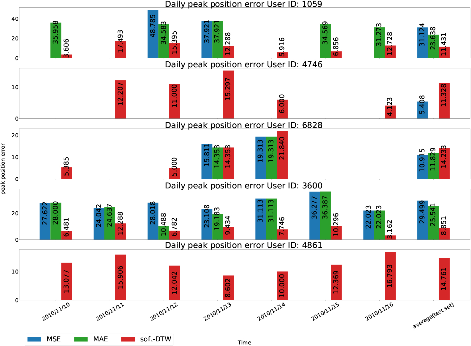

Figure 8.

Daily peak position error with MSE, MAE, soft-DTW loss functions.

3.3 Evaluation on CER dataset

Figure 6 and Table 4 demonstrate these four scenarios on the test set, showcasing significant improvements in peak prediction for all these five residential buildings with the soft-DTW loss function: the number of successful peak predictions in the True Positive case (green in Fig. 6) is notably increased compared to the MAE and MSE loss functions; similarly, all five residential buildings experience a significant reduction of Type Error II (red in Fig. 1) with the soft-DTW loss function; the True Negative case (grey in Fig. 6) is slightly improved, with only one day missing. Nevertheless, for the False Positive (Type Error I), the soft-DTW loss function tends to overestimate compared to the other loss functions, which will be discussed in the next section for potential enhancement.

Deploying the Eqs (4) and (5) for the case TP, daily peak position error and daily peak load error are shown in Fig. 8 and Fig. 7 respectively.

In terms of peak load error, soft-DTW presents fairly good results for all these five buildings. Although the MAE loss function performs slightly better than soft-DTW for building ID: 3600, the difference is relatively small.

Three out of the five residential buildings (ID: 1059, ID: 3600, ID: 4861) achieve the lowest peak position error with the soft-DTW loss function. The remaining two buildings (ID: 4746 and ID: 6828) exhibit better performance in terms of peak position error with the MSE loss function. This could be attributed to two possible reasons. Firstly, the number of valid days for the True Positive case with the MSE loss function is lower than that of the soft-DTW loss function for these two buildings. Secondly, the soft-DTW loss function emphasizes the shape of the curves, which may focus less on time deformation and result in peak position errors. Thus, these results lead us to consider combining the advantages of the MSE loss function and the soft-DTW loss function. In the next part, different combined loss functions will be compared and analyzed on the same dataset.

4. Part III: Combined soft-DTW loss functions

In the previous section, we observed a significant improvement in peak prediction using the soft-DTW loss function. However, we also noticed that the model using soft-DTW may be overestimated with higher Type Error I, and some residential buildings exhibit higher peak position errors. Therefore, we would like to investigate whether combining the soft-DTW loss function with other loss functions can lead to further improvements in these areas.

4.1 soft-DTW $+$ MAE/MSE

The combined soft-DTW loss functions with MSE and MAE is defined as a linear combination with a hyperparameter $\alpha\in[0,1]$ :

$\displaystyle L_{\textit{DTW}_{\gamma}-\textit{MSE}}(\hat{\bm{y}},\bm{y})$

(6) $\displaystyle=\alpha\textit{DTW}_{\gamma}(\hat{\bm{y}},\bm{y})+(1-\alpha)% \textit{MSE}(\hat{\bm{y}},\bm{y})$ $\displaystyle L_{\textit{DTW}_{\gamma}-\textit{MAE}}(\hat{\bm{y}},\bm{y})$ (7) $\displaystyle=\alpha\textit{DTW}_{\gamma}(\hat{\bm{y}},\bm{y})+(1-\alpha)% \textit{MAE}(\hat{\bm{y}},\bm{y})$

Figure 9.
Residential loads predictions with soft-DTW, soft-DTW 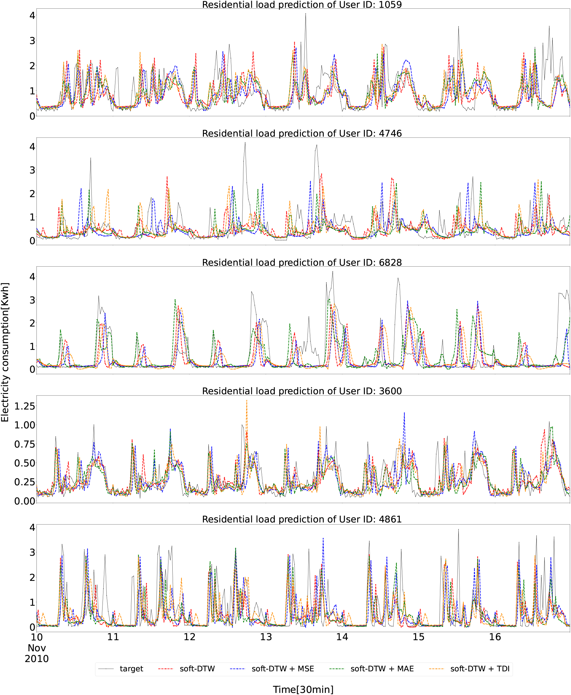$+$ MSE, soft-DTW $+$ MAE, soft-DTW $+$ TDI loss functions from 2010-11-10 to 2010-11-16.

Figure 10.
Confusion matrix of peak performance of combined loss functions on test set.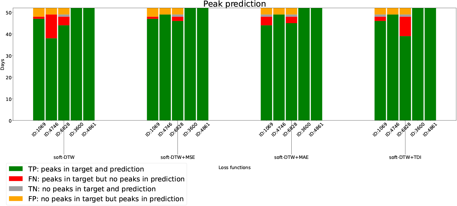

Figure 11.
Average performance on the test set.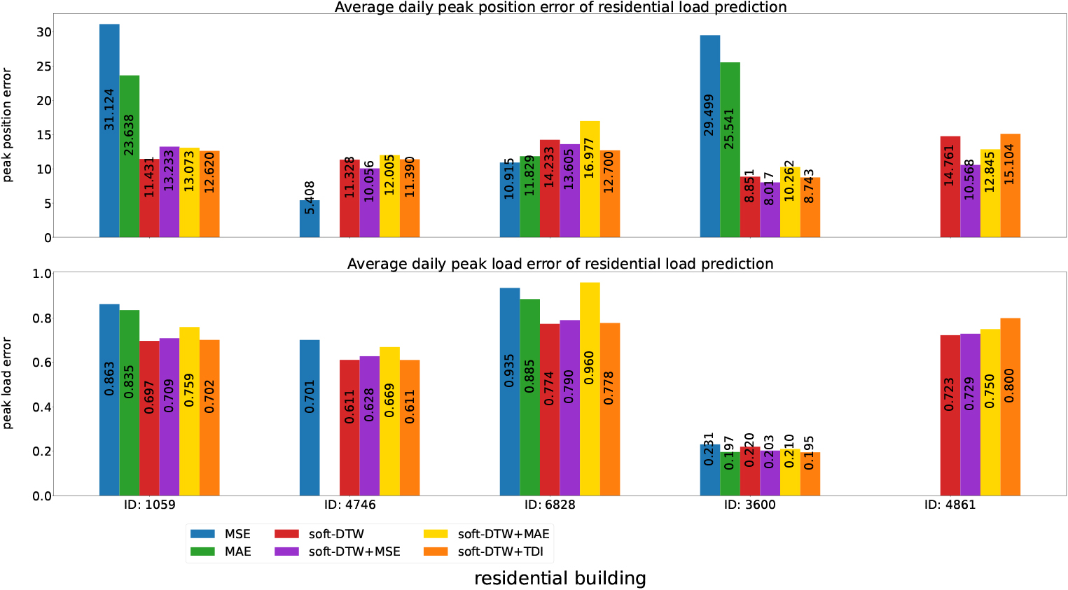

4.2 DILATE: Soft-DTW $+$ time distortion index

Another combined formula has been proposed in the literature by Le Guen and Thome [28], who introduced a time distortion index as a novel penalization term for the soft-DTW loss function. The time distortion index is defined as the inner product of the optimal alignment $\bm{A}^{*}$ and penalization matrix $\bm{D}$ :

$\displaystyle\textit{TDI}(\hat{\bm{y}},\bm{y})=\langle\bm{A}^{*},\bm{D}\rangle$ (8)

where

$\displaystyle\bm{D}_{i,j}=\frac{(i-j)^{2}}{n}$

The matrix $\bm{D}$ penalizes the optimal alignment for not being diagonal. Based on this definition, the more delay of the peak, the more penalization of the alignment.

In order to make TDI differentiable everywhere, they replaced the optimal alignment $\bm{A}^{*}$ with a smoothed average alignment $\bm{A}_{\gamma}^{*}$ which is the gradient of soft-DTW in Eq. (2.1):

$\displaystyle A_{\gamma}^{*}=\nabla_{\Delta}\textit{DTW}_{\gamma}(\hat{\bm{y}}% ,\bm{y})$ $\displaystyle=\frac{\sum\limits_{\bm{A}\in\mathcal{A}_{N,M}}\exp\left(-\frac{% \langle\bm{A},\Delta(\hat{\bm{y}},\bm{y})\rangle}{\gamma}\right)\bm{A}}{\sum% \limits_{\bm{A}\in\mathcal{A}_{N,M}}\exp\left(-\frac{\langle\bm{A},\Delta(\hat% {\bm{y}},\bm{y})\rangle}{\gamma}\right)}$ (9)

Then the combined soft-DTW with TDI, namely DILATE is defined:

$\displaystyle L_{\textit{DILATE}}(\hat{\bm{y}},\bm{y})$ $\displaystyle=\alpha\textit{DTW}_{\gamma}(\hat{\bm{y}},\bm{y})+(1-\alpha)% \textit{TDI}_{\gamma}(\hat{\bm{y}},\bm{y})$ (10) $\displaystyle=\alpha\textit{DTW}_{\gamma}(\hat{\bm{y}},\bm{y})+(1-\alpha)% \langle\bm{A}_{\gamma}^{*},\bm{D}\rangle$

4.3 Comparison of different combined soft-DTW loss functions on CER dataset

To ensure a fair comparison, we followed the same procedure as in the previous section, with all combined loss functions set to $\alpha=0.5$ . The prediction results from 2010-11-10 to 2010-11-16 are shown in Fig. 9.

Table 5
Confusion matrix of peak performance of combined loss functions on test set

Days	Soft-DTW					Soft-DTW $+$ MSE					Soft-DTW $+$ MAE					Soft-DTW $+$ TDI
	1059	4746	6828	3600	4861	1059	4746	6828	3600	4861	1059	4746	6828	3600	4861	1059	4746	6828	3600	4861
TP	47	38	44	52	52	47	49	46	52	52	44	49	45	52	52	46	49	39	52	52
FN	1	11	4	0	0	1	0	2	0	0	4	0	3	0	0	2	0	9	0	0
TN	0	0	1	0	0	0	0	1	0	0	1	0	1	0	0	1	0	1	0	0
FP	4	3	3	0	0	4	3	3	0	0	3	3	3	0	0	3	3	3	0	0

It can be observed that all of the combined loss functions are able to predict most of the peaks, surpassing the performance of the MSE and MAE loss functions. Despite the lower Type II error observed with the combined loss functions, the confusion matrix (Fig. 10) and Table 5 reveal that there is no substantial improvement in reducing Type I error, contrary to the initial expectations.

Regarding the peak position error, as shown in Fig. 11, our expectations are met with the MSE combined loss function, as four out of five residential buildings show a slight decrease in peak position errors. However, the MAE and TDI combined loss functions do not exhibit a consistent improvement across all buildings.

It is worth noting that all combined loss functions result in higher errors for peak load. This can be attributed to the hyperparameter $\alpha=0.5$ , which reduces the ability of the soft-DTW component to accurately capture the peaks. Therefore, the higher errors in peak load are reasonable and expected given the reduction in peak capturing ability.

5. Conclusions

This paper presents a comprehensive comparison of different loss functions, including soft-DTW and its combined formulas, for short-term residential load forecasting with a specific focus on peak prediction evaluation. Additionally, a novel evaluation methodology is introduced, which involves the use of confusion matrix and new errors for peak position and peak load.

The comparison results indicate that using MSE or MAE as default loss functions for short-term load forecasting may not be optimal when dynamics and peak values are of greater importance. Soft-DTW loss function and its combined formula perform largely better than MSE and MAE loss functions in terms of peak prediction performance. However, the combined loss functions with MAE and TDI do not show a consistent improvement across all buildings. Even though the combined soft-DTW loss function with MSE shows a slight reduction in peak position error, the difference compared to soft-DTW alone is relatively small. To gain deeper insights into these issues, the utilization of landscape visualization for these loss functions holds great potential. We intend to pursue these investigations in our future studies.

References

Ajaz

Bernell

. Microgrids and the transition toward decentralized energy systems in the United States: A Multi-Level Perspective. Energy Policy. 2021; 149: 112094.

Yoldaş

Önen

Muyeen

Vasilakos

Alan

. Enhancing smart grid with microgrids: Challenges and opportunities. Renewable and Sustainable Energy Reviews. 2017; 72: 205–214.

Zhao Magoulès

. A review on the prediction of building energy consumption. Renewable and Sustainable Energy Reviews. 2012; 16(6): 3586–3592.

Runge

Zmeureanu

. Forecasting energy use in buildings using artificial neural networks: A review. Energies. 2019; 12(17): 3254.

Fan

Wang

Gang

. Assessment of deep recurrent neural network-based strategies for short-term building energy predictions. Applied Energy. 2019; 236: 700–710.

Hippert

Pedreira

Souza

. Neural networks for short-term load forecasting: A review and evaluation. IEEE Transactions on Power Systems. 2001; 16(1): 44–55.

Almalaq

Edwards

. A review of deep learning methods applied on load forecasting. In 2017 16th IEEE International Conference on Machine Learning and Applications (ICMLA). IEEE. 2017. pp. 511–516.

Lara-Benítez

Carranza-García

Riquelme

. An experimental review on deep learning architectures for time series forecasting. International Journal of Neural Systems. 2021; 31(03): 2130001.

. Load forecasting via deep neural networks. Procedia Computer Science. 2017; 122: 308–314.

10.

Sheng

Wang

Chen

Zhou

Sun

. Convolutional residual network to short-term load forecasting. Applied Intelligence. 2021; 51(4): 2485–2499.

11.

Shi

. Deep learning for household load forecasting – A novel pooling deep RNN. IEEE Transactions on Smart Grid. 2017; 9(5): 5271–5280.

12.

Wang

Liu

Bao

Zhang

. Short-term load forecasting with multi-source data using gated recurrent unit neural networks. Energies. 2018; 11(5): 1138.

13.

Acharya

Y-M

Lee

. Short-term load forecasting for a single household based on convolution neural networks using data augmentation. Energies. 2019; 12(18): 3560.

14.

Dorado Rueda

Durán Suárez

del Real Torres

. Short-term load forecasting using encoder-decoder wavenet: Application to the french grid. Energies. 2021; 14(9): 2524.

15.

Marino

Amarasinghe

Manic

. Building energy load forecasting using deep neural networks. In IECON 2016-42nd Annual Conference of the IEEE Industrial Electronics Society. IEEE. 2016. pp. 7046–7051.

16.

Lusis

Khalilpour

Andrew

Liebman

. Short-term residential load forecasting: Impact of calendar effects and forecast granularity. Applied Energy. 2017; 205: 654–669.

17.

Wang

Zhu

. An effective deep learning neural network model for short-term load forecasting. Concurrency and Computation: Practice and Experience. 2020; 32(7): 5595.

18.

Dudek

. Short-term load forecasting using neural networks with pattern similarity-based error weights. Energies. 2021; 14(11): 3224.

19.

Sakoe

Chiba

. Dynamic programming algorithm optimization for spoken word recognition. IEEE Transactions on Acoustics, Speech, and Signal Processing. 1978; 26(1): 43–49.

20.

Aghabozorgi

Shirkhorshidi

Wah

. Time-series clustering – a decade review. Information Systems. 2015; 53: 16–38.

21.

Cuturi

Blondel

. Soft-dtw: a differentiable loss function for time-series. In International Conference on Machine Learning. PMLR. 2017. pp. 894–903.

22.

Wolf

Chin

Baker

. Unsupervised data-driven automotive diagnostics with improved deep temporal clustering. In 2019 IEEE 90th Vehicular Technology Conference (VTC2019-Fall). IEEE. 2019. pp. 1–6.

23.

Liang

Tang

. Fuzzy Clustering Based Scenario Reduction for Stochastic Day-Ahead Scheduling in Power Systems. In 2020 IEEE Power & Energy Society General Meeting (PESGM). IEEE. 2020. pp. 1–5.

24.

Tang

Bai

. Datsing: Data augmented time series forecasting with adversarial domain adaptation. In Proceedings of the 29th ACM International Conference on Information & Knowledge Management. 2020. pp. 2061–2064.

25.

Kontogiannis

Bargiotas

Daskalopulu

Tsoukalas

. A meta-modeling power consumption forecasting approach combining client similarity and causality. Energies. 2021; 14(19): 6088.

26.

Flor Ambrosi

Herraiz Jaramillo

Contreras

. Definition of Residential Power Load Profiles Clusters Using Machine Learning and Spatial Analysis. Energies. 2021; 14(20): 6565.

27.

K-H

Huang

P-S

I-C

Wang

F-J

. Prediction of Time Series Data Based on Transformer with Soft Dynamic Time Wrapping. In 2020 IEEE International Conference on Consumer Electronics-Taiwan (ICCE-Taiwan). IEEE. 2020. pp. 1–2.

28.

Le Guen

Thome

. Shape and time distortion loss for training deep time series forecasting models. Advances in Neural Information Processing Systems. 2019; 32.

29.

Zhang

Thorburn

. A dual-head attention model for time series data imputation. Computers and Electronics in Agriculture. 2021; 189: 106377.

30.

Shi

Fang

Zhu

. An Improved attention-based integrated deep neural network for PM2.5 concentration prediction. Applied Sciences. 2021; 11(9): 4001.

31.

Singh

Gao

Lizotte

. On hourly home peak load prediction. In 2012 IEEE Third International Conference on Smart Grid Communications (SmartGridComm). IEEE. 2012. pp. 163–168.

32.

Milojković

Litovski

. ANN application for the next day peak electricity load prediction. In 11th Symposium on Neural Network Applications in Electrical Engineering. IEEE. 2012. pp. 237–241.

33.

Lee

G-C

. Regression-Based Methods for Daily Peak Load Forecasting in South Korea. Sustainability. 2022; 14(7): 3984.

34.

Bellman

Kalaba

. On adaptive control processes. IRE Transactions on Automatic Control. 1959; 4(2): 1–9.

35.

Noering

FK-D

Schroeder

Jonas

Klawonn

. Pattern discovery in time series using autoencoder in comparison to nonlearning approaches. Integrated Computer-Aided Engineering. 2021; 28(3): 237–256.

36.

Goodfellow

Bengio

Courville

. Deep Learning. Cambridge, MA, USA: MIT Press. 2016.

37.

Zhang

Ren

Sun

. Deep residual learning for image recognition. In Proceedings of the IEEE Conference on Computer Vision and Pattern Recognition. 2016. pp. 770–778.

38.

Taylor

Studer

Goldstein

. Visualizing the loss landscape of neural nets. Advances in Neural Information Processing Systems. 2018; 31.

39.

Kiprijanovska

Stankoski

Ilievski

Jovanovski

Gams

Gjoreski

. Houseec: Day-ahead household electrical energy consumption forecasting using deep learning. Energies. 2020; 13(10): 2672.

40.

Gong

Mahato

Sun

Chen

Wen

. Research on short-term load prediction based on Seq2seq model. Energies. 2019; 12(16): 3199.

41.

Wang

Chen

Zeng

Kong

Sun

Guo

Liu

. Short-term load forecasting for industrial customers based on TCN-LightGBM. IEEE Transactions on Power Systems. 2020; 36(3): 1984–1997.

42.

Cheng

Mashima

Thing

. PowerLSTM: power demand forecasting using long short-term memory neural network. In International Conference on Advanced Data Mining and Applications. Springer. 2017. pp. 727–740.

43.

Wen

Zhou

Yang

. Load demand forecasting of residential buildings using a deep learning model. Electric Power Systems Research. 2020; 179: 106073.

44.

Kong

Dong

Jia

Hill

Zhang

. Short-term residential load forecasting based on LSTM recurrent neural network. IEEE Transactions on Smart Grid. 2017; 10(1): 841–851.

45.

Mocanu

Nguyen

Gibescu

Kling

. Deep learning for estimating building energy consumption. Sustainable Energy, Grids and Networks. 2016; 6: 91–99.

46.

Repository

UML

. Individual household electric power consumption Data Set. https://archive.ics.uci.edu/ml/datasets/individual+household+electric+power+consumption.

47.

Commission for Energy Regulation (CER). CER Smart Metering Project – Electricity Customer Behaviour Trial, 2009–2010 [dataset]. 1st Edition. Irish Social Science Data Archive. SN: 0012-00. 2012. https://www.ucd.ie/issda/data/commissionforenergyregulationcer/.

48.

Petitjean

Ketterlin

Gançarski

. A global averaging method for dynamic time warping, with applications to clustering. Pattern Recognition. 2011; 44(3): 678–693.

49.

Nagi

Yap

Nagi

Tiong

Ahmed

. A computational intelligence scheme for the prediction of the daily peak load. Applied Soft Computing. 2011; 11(8): 4773–4788.

50.

Zhu

Mao

Yan

. LSTM enhanced by dual-attention-based encoder-decoder for daily peak load forecasting. Electric Power Systems Research. 2022; 208: 107860.

Enhancing peak prediction in residential load forecasting with soft dynamic time wrapping loss functions

Abstract

Keywords

1. Introduction

2.1 soft-DTW

2.2.1 Residual block with skip connections

2.2.3 Validation on benchmark dataset

Table 1 One-day-ahead prediction with 15 min resolution

Table 2 MSE and MAE on test set for different loss functions

Table 3 Confusion matrix of peak prediction

4. Part III: Combined soft-DTW loss functions

4.1 soft-DTW + MAE/MSE

Table 5 Confusion matrix of peak performance of combined loss functions on test set

References

Table 1
One-day-ahead prediction with 15 min resolution

Table 2
MSE and MAE on test set for different loss functions

Table 3
Confusion matrix of peak prediction

4.1 soft-DTW $+$ MAE/MSE

Table 5
Confusion matrix of peak performance of combined loss functions on test set