Neural architecture search for radio map reconstruction with partially labeled data

Abstract

In this paper, we tackle the challenging task of reconstructing Received Signal Strength (RSS) maps by harnessing location-dependent radio measurements and augmenting them with supplementary data related to the local environment. This side information includes city plans, terrain elevations, and the locations of gateways. The quantity of available supplementary data varies, necessitating the utilization of Neural Architecture Search (NAS) to tailor the neural network architecture to the specific characteristics of each setting.

Our approach takes advantage of NAS’s adaptability, allowing it to automatically explore and pinpoint the optimal neural network architecture for each unique scenario. This adaptability ensures that the model is finely tuned to extract the most relevant features from the input data, thereby maximizing its ability to accurately reconstruct RSS maps. We demonstrate the effectiveness of our approach using three distinct datasets, each corresponding to a major city. Notably, we observe significant enhancements in areas near the gateways, where fluctuations in the mean received signal power are typically more pronounced. This underscores the importance of NAS-driven architectures in capturing subtle spatial variations. We also illustrate how NAS efficiently identifies the architecture of a Neural Network using both labeled and unlabeled data for Radio Map reconstruction. Our findings emphasize the potential of NAS as a potent tool for improving the precision and applicability of RSS map reconstruction techniques in urban environments.

Keywords

Neural networks with optimized architecture radio map reconstruction learning with partially labeled data

1. Introduction

Retrieving the exact position of the connected objects has become an important feature of the Internet of Things (IoT). Such connected objects have indeed been widespread over the last few years thanks to the low cost of the radio integrated chips and sensors and their possibility of being embedded in plurality of the devices.

By this they can help in fast development of large-scale physical monitoring and crowdsensing systems (like smart cities, factories, transportation, etc.). For the location-dependent application and services these abilities to associate accurate location with physical data gives huge opportunities [1]. For example, the fine-grain and dynamic update of air pollution and/or weather maps could benefit from geo-referenced mobile sensing1

¹
https://sarws.eu/.

(e.g., aboard taxis, buses, bicycles…), thus continuously complementing the data from static stations. One of the localization techniques is Global Positioning System (GPS) which has been widely used over the past decades. More recently, low-cost advanced GPS solutions were proposed (like RTK, Bi-band,..), but still they suffer from high energy consumption which is not suitable for IoT applications.

As an alternative, one can opportunistically measure location-dependent radio metrics, like Received Signal Strength (Indicator) (RSSI), Time (Difference) of Arrival, Angle of Arrival, etc., because these sensor nodes communicate with one/several gateways at the same time (e.g. while sending a packet to the infrastructure to store this data in the cloud/server). Based on these metrics, there exist several methods to determine the node position: trilateration, triangulation, proximity detection, or fingerprinting [2, 3, 4]. We will focus on the last approach – fingerprinting [5] – which requires (ideally) full map of mentioned above radio metrics, covering the zone of interest. However, collecting metrics in each point of the zone of interest is impractical and time costly in real-world scenarios, therefore most approaches rely on sparse and non-uniformly distributed measurements.

In this sense, classical map interpolation techniques such as RBF[6, 7, 8] or kriging [9, 10] are used. Although these methods are relatively fast, they are quite weak in retrieving and predicting the complex and heterogeneous spatial patterns that are usually observed in real life signals (e.g., sudden and/or highly localized transient variations in the received radio metric due to specific environmental, local or topological effects). Another approach consists on deterministic simulation such as Ray-Tracing tools [11, 12, 13, 14]. Given some real field measurements and then calibrated over them, these models predict the radio propagation while simulating electromagnetic interactions with the environment. These technologies, however, need a complete description of the environment (properties of the materials of the obstacles, buildings, shape,etc.). Moreover, they are computationally complex, and in case of minor changes in the local area, these simulations should be re-run again. Recently, studies have employed machine learning for this task by considering radio maps as images and adapting neural network models that have been proposed for image completion. These models are based on the fully generated dataset by Ray-Tracing tools for predicting the signal propagation given the buildings mask and position of the transmitter [15]; or predicting the received power value for the Long Term Evolution (LTE) of the signal with use of additional information and neural networks [16, 17] with handcrafted structures.

In this work we will focus on the received signal strength map reconstruction, where only small amount of ground truth GPS-tagged measurements are available preventing to use existing NN models with handcrafted architectures and for which Ray-Tracing models could not be applied due to the lack of information about physical properties of the environment or due to high computational complexity. Our approach is based on Neural Architecture Search (NAS) [18] which aims to find an optimized NN model for this task. We show that by employing the latter technique, it is feasible to learn model parameters while simultaneously exploring the architecture. In addition, we employ unlabeled data in conjunction with ground-truth measurements in the training phase, as well as side information that accounts for the existence of buildings, to obtain knowledge and improve the model’s performance. We assess our technique using three RSSI Map reconstruction collections, including one we produced for the city of Grenoble in France. In the case of the latter, we thoroughly examine its properties. In particular, we show that unlabeled data can effectively be used to find an efficient optimized NN model and that the side information provides valuable knowledge for learning. The obtained model is shown to have generalization ability on base stations that were not used in the training phase. The contribution of this paper is twofold:

•

We propose a unified framework with the use of side information, for which we study the generalization ability of a neural network model which architecture is optimized over labeled and unlabeled data using side-information. This is an extension of the work of [19, 20].

•

Furthermore, we provide empirical evaluation over three large-scale RSSI collections showing that the proposed approach is highly competitive compared to the state-of-the-art models in terms of quality metrics.

2. Related state of the art

Classical techniques such as radial basis functions (RBF) or kriging [5] are simple and fast, but they are poor at predicting the complex and heterogeneous spatial patterns commonly observed in real-world radio signals (e.g., sudden and/or highly localized transient variations in the received signal due to specific environmental or topological effects, such as specific building shapes, presence of public furniture, ultra-navigation, etc.). Furthermore, data augmentation approaches for artificially increasing the number of measurements in radio map reconstruction issues have been developed.

The goal is to use the synthetic data created as extra data to train complex map interpolation models. However, these techniques need a highly thorough description of the physical environment and are unable to predict dynamic changes in the environment over time. A key bottleneck is their high computational complexity.

In the following, we go through some more relevant work on RSSI map reconstruction, including interpolation and data-augmentation techniques, as well as machine learning approaches.

2.1 Interpolation and data-augmentation techniques

Kriging or Gaussian process regression [21] is a prominent technique for radio map reconstruction in the wireless setting that takes into consideration the distance information between supplied measured locations while attempting to uncover their underlying 2D dependency.

Radial basis functions (RBF) [5, 8, 6] are another approach that simply considers the dependent on the distance between observed locations. As a result, this method is more adaptive and has been found to be more tolerant to some uncertainty [22]. Furthermore, in order to compare the performance of the RBF with different kernel functions for the map reconstruction of signal strength of Long Range (LoRa) radio waves, [5] divided all of the points in a database of outdoor RSSI measurements into training and testing subsets, with the linear kernel showing the best accuracy in both standard deviation and considered metric. The two approaches stated above (which depend on kernel techniques and underlying spatial relationships of the input measurements) need a lot of input data to provide reliable interpolation results, making them sensitive to sparse training sets. These methods have consequently been considered in pair with crowdsensing, where, for example in [10], to improve the performance of basic kriging, one calls for measuring the radio metric in new points/cells where the predicted value is still presumably imprecise. A quite similar crowdsensing method has also been applied in [23] after considering the problem as a matrix completion problem using singular value thresholding, where it is possible to ask for additional measurements in some specific cells where the algorithm has a low confidence in the predicted result. In our case though, we assume that we can just rely on a RSSI map with few ground-truth initial RSSI measurements.

Another approach considered in the context of indoor wireless localization (with map reconstruction firstly) relies on both measured field data and an a priori path loss model that accounts for the effect of walls presence and attenuation between the transmitter and the receiver [24] by using the wall matrix, which counts the number of walls along the path from the access point to the mobile location and penalize value according to that number. In some outdoor settings, training points are divided into a number of clusters of measured neighbors having specific RSSI distributions, and local route loss models are applied in an effort to capture localized wireless topology effects in each cluster [25]. However as parametric path loss models are usually quite imprecise, these techniques have a limited generalization capabilities and require additional impractical in-site (self-)calibration. A quite similar approach, except the use of additional side information, is followed in [26], where they propose an algorithm called SateLoc. Based on satellite images, it is then suggested to perform a segmentation of the areas “crossed” by a given radio link, depending on their type (e.g., terrain, water, forest, etc.). Then, proportionally to the size of the crossed region(s), power path loss contributions are computed according to a prior model parameters (i.e., associated with each environment type) and summed up to determine the end-to-end path loss value.

One more way to build or complete radio databases stipulated in the context of fingerprinting based positioning consists in relying on deterministic simulation approach, namely Ray-Tracing tools (e.g., [13, 27, 28, 14, 12]). This technique aim at predicting in-site radio propagation (i.e., simulating electromagnetic interactions of transmitted radio waves within an environment). Once calibrated with a few real field measurements, such simulation data can relax initial metrology and deployment efforts (i.e., the number of required field measurements) to build an exploitable radio map, or even mitigate practical effects that may be harmful to positioning, such as the cross-device dispersion of radio characteristics (typically, between devices used for offline radio map calibration and that used for online positioning). Nevertheless, these tools require a very detailed description of the physical environment (e.g., shape, constituting materials and dielectric properties of obstacles, walls…). Moreover, they are notorious for requiring high and likely prohibitive computational complexity in real applications. Finally, simulations must be re-run again, likely from scratch, each time minor changes are introduced in the environment, e.g. the impact of human activity (like changing crowd density, temporary radio link obstructions).

2.2 NN based models trained after data augmentation

There is an increasing interest in applying machine and deep learning methods to the problem of RSSI map reconstruction. These approaches have shown an ability to capture unseen spatial patterns of local effects and unseen correlations. Until now, to the best of our knowledge, these algorithms were primarily trained over simulated datasets generated by data-augmentation approaches (that were mentioned above).

In [15], given a urban environment, city geography, transmitter (Tx) location, and optionally pathloss measurements and car positions the authors introduce a UNet-based neural network called RadioUNet in the supervised learning setting, which outputs radio path loss estimates trained on a large set of generated using the Dominant Path Model data [29].

The authors of [30] propose a two-phase transfer learning with Generative Adversarial Networks (GAN) , which comprises two stages, to estimate the power spectrum maps in the underlay cognitive radio networks. The domain projecting (DP) framework is used to first project the source domain onto a neighboring domain. The target domain’s entire map is then rebuilt or reconstructed using the domain completing framework and the recovered features from the surrounding domain.

For training of the DP, fully known signal distribution maps have been used. In another contribution, to improve the kriging predictions the authors have used the feedforward neural network for path loss modelling [31], as conventional parametric path loss models has a small number of parameters and do not necessarily consider shadowing besides mean power attenuation.

Apart from wireless applications, similar problems of map reconstruction also exist in other domains. In [32] for instance, the goal is to create the full topographic maps of mountains area given sparse measurements of the altitudes values. For this purpose, they use a GAN architecture, where in the discriminator they compare pairs of the input data and the so-called “received” map, either generated by the generator or based on the given full true map. In other work [33] the authors estimate the sea surface temperature with use of GAN architecture in the unsupervised settings but having a sequence of corrupted observations (with different cloud coverage) and known mask distribution. Another close more general problem making extensive use of neural networks is the image inpainting problem, where one needs to recover missing pixels in a single partial image. By analogy, this kind of framework could be applied in our context too, by considering the radio map as an image, where each pixel corresponds to the RSSI level for a given node location. It has been shown in [19] the interpretation of collected measurements on a map as an image with some pixels gives overall better result. But the problem is in consumed time as it does not give the generalized model and do not use the additional information about the local environment. Usually, such image inpainting problems can be solved by minimizing a loss between true and estimated pixels, where the former are artificially and uniformly removed from the initial full image. This is, however, not possible and not realistic in our case, as only a few ground-truth field measurements collected on the map can be used to reconstruct the entire image.

In contrast to the previous approaches, in our study we consider practical situations where data-augmentation techniques cannot be used, mainly because of unknown environment characteristics and computational limitations, and where only a small amount of collected ground-truth measurements is available.

Finally, a few contributions aim at predicting the received power value based on neural networks and additional information. For instance, in [16, 17, 34], RSS values are predicted in exact points, given meta information such as the radio characteristics (e.g., transmission specifications or relationship between the receiver (Rx) and the transmitter (Tx), like horizontal/vertical angle, mechanical/electrical tilt angle, 2D/3D distance, base station antenna orientation, etc.) and/or prior information about the buildings (e.g., height and presence). In case the latter information is missing, predictions can be made also by means of satellite images (e.g., paper [34]). In these papers though, the map reconstruction cannot be performed directly. As the prediction is realized for each point separately, it is thus time consuming. Moreover, the authors do not take into account the local signal values, but only the physical parameters and physical surroundings (similarly to standard path loss models).

2.3 Semi-supervised learning

The constitution of coherent and consistent labeled collections are often done manually. This necessitates tremendous effort, which is generally time consuming and, in some situations, unrealistic. The learning community has been looking at the concept of semi-supervised learning for discrimination and modeling tasks since the end of the 1990s, based on the observation that labeled data is expensive while unlabeled data is plentiful and contains information on the problem we are trying to solve.

The three main families of Semi-supervised Learning (SSL) approaches are Generative, Graph-based and Discriminant methods [35].

Generative methods: Semi-supervised learning with generative models involves estimating the conditional density using a maximum likelihood technique to estimate the parameters of the model. In this case, the hidden variables associated with the labeled examples are known in advance and correspond to the class of these examples. The basic hypothesis of these models is that if two examples are in the same group, then they are likely to belong to the same class [36]. We can thus interpret semi-supervised learning with generative models $(a)$ as a supervised classification where we have additional information on the probability density of the data, or $(b)$ as a partition with additional information on the class labels of a subset of examples [37, 38]. If the hypothesis generating the data is known, generative models can become very powerful [39].

Graph-based methods: Graph-based methods employ an empirical graph built on the labeled and unlabeled examples to express their geometry [40]. They are based on the hypothesis that if two examples are in the same group, then they are likely to belong to the same class. The nodes of this graph represent the training examples and the edges translate the similarities between the examples. These similarities are usually given by a positive symmetric matrix, where the weight between two nodes is non-zero if and only if the corresponding examples are connected.

Methods for Semi-Supervised Learning leverage generative and graph-based approaches to harness the underlying data geometry through density estimation techniques or distance-based similarity matrix construction. However, these methods have their limitations when the underlying distributional assumptions become invalid or the distance used to estimate the similarity matrix fails to accurately represent the true data topology. In such cases, their performance tends to degrade in comparison to scenarios where only labeled examples are used for model training [41].

Discriminant methods: To address these shortcomings, researchers have been motivated to devise strategies for mitigating these issues. One such approach involves using predictions from a discriminant model on unlabeled data to assign pseudo-labels. These pseudo-labeled examples are then integrated into the training process in a technique known as self-training [42, 43]. This iterative self-training process involves the repeated steps of pseudo-labeling and training a new model until there are no more unlabeled examples left. Some approaches have tackled the problem of modelling noise in the pseudo-labeling phase [44]. furthermore, in the case where class pseudo-labels are assigned to unlabeled examples, by thresholding the outputs of the classifier corresponding to these examples, it can be shown that the self-learning algorithm works according to the clustering assumption [45].

2.4 Neural architecture search

The creation and selection of features in many tasks are done manually in general; this critical phase for some conventional machine learning algorithms might be time-consuming and costly. Neural Networks address this challenge by learning feature extractors in an end-to-end manner. These feature extractors, on the other hand, rely on architectures that are still manually constructed, and with the rapid development of deep learning, designing an appropriate NN model has become onerous in many cases.

This problem has recently been addressed by a new field of research called (NAS) [18, 46, 47, 48]. In a variety of applications, such as image segmentation and classification, Neural Networks with automatically found architectures have already outperformed “conventional” NN models with hand-crafted structures.

Different types of existing methods of search are described below. In the last few years the research on the topic of NAS has been shown a huge interest in the different fields. Among various studies, there are different techniques that are based on divers methods like Reinforcement Learning [49], Evolutionary Algorithm [50] or Bayesian Optimization [51]. Recently gradient-based methods became more popular. For example, one of the first methods based on this technique was presented in [52] and is called Differentiable Architecture Search (DARTS), which is using relaxation to, at the same time, optimize the structure of a cell, and the weight of the operations relative to each cell. After finding the best combinations, blocks are stacked manually to produce a neural network. Based on DARTS, more complex methods have appeared such as AutoDeepLab [53] in which a network is optimized at 3 levels : $(i)$ the parameters of the operations, $(ii)$ the cell structure and $(iii)$ the macro-structure of the network that is stacked manually. Despite the fact that a complex representation leads to powerful architectures, this technique has some drawbacks, such as the fact that the generated architecture is single-path, which means it does not fully exploit the representation’s capabilities. Moreover, as the search phase is done over a fixed network architecture, it might not be the same between different runs, thus it is complicated to use transfer learning and the impact of training from scratch can be significant. To overcome these limitations, one possible technique is to use Dynamic Routing as proposed in [54]. This approach is different from the traditional gradient based methods proposed for NAS in the sense that it does not look for a specific fixed architecture but generates a dynamic path in a mesh of cells on the fly without searching by weighting the paths during training procedure.

In the context of signal strength map reconstruction with neural networks, the choice between using a Generic Algorithm and Dynamic Routing to automatically find the architecture of the neural network depends on the specific problem, dataset, and constraints. Genetic Algorithms are well-suited for exploring a large and complex search space of neural network architectures [55]. They work by evolving a population of potential solutions over multiple generation, allowing them to efficiently search for a wide range of architectures [56]. This is important in signal strength map reconstruction where the optimal architecture may not be known in advance and can vary based on the nature of the signals, the environment, and other factors. Genetic Algorithms maintain diversity within the population of neural network architectures, ensuring that a wide range of designs is considered. This can be beneficial in finding novel and effective solutions that might be missed by more deterministic methods like Dynamic Routing as it has been shown in [19].

In our study, we look at how well neural networks can extract complex features and their relationships to signal strength in the local area or under similar conditions, as well as their ability to take into account additional environmental information without having access to more complex physical details. This is performed through a search for a model with an optimized architecture adapted to the task with partially labeled data. From this perspective and following [19], we consider the genetic algorithm for NAS.

3. Application to the stated RSS map reconstruction problem

Additional information could be represented in different manners, and they could be included into the algorithm in a variety of ways, such as independent channels, parallel channels inputs, directly in the learning goal, or in the ranking metric during model selection. We adapted the proposed algorithm presented in [20] for multi-channel input by combining additional context information with the data in the model’s input; and we assessed the model’s performance on unseen base stations that were not utilized in the learning process.

Here, we suppose to have a small set of $n$ available base stations $(X^{j})_{1\leqslant j\leqslant n}$ . For each given matrix of base station $X^{j};j\in\{1,\ldots,n\}$ , let $Y^{j}\in\mathbb{R}^{H\times W}$ be its corresponding 2D matrix of signal strength values measurements, where $H\times W$ is the size (in number of elements in a grid) of the zone of interest.

In practice, we have access only to some ground truth measurements $Y^{j}_{m}$ , meaning that

$\displaystyle Y^{j}_{m}=∼{}Y^{j}\odot M^{j},$ (1)

with $M^{j}\in\{0,1\}^{H\times W}$ a binary mask of available measurements, and $\odot$ is the element-wise product of two matrices of the same dimensions, also called the Hadamard’s product. Here we suppose sparsity meaning that the number of non-null elements in $Y^{j}_{m}$ is much lower than the overall size $H\times W$ . For each base station $X^{j}$ we estimate unknown measurements $\tilde{Y}_{u}^{j}$ in $Y^{j}$ with a RBF interpolation given $(X^{j}_{m},Y^{j}_{m})$ , so that we have a new subset $(X^{j}_{u},\tilde{Y}^{j}_{u})$ , where $X^{j}_{m}=X^{j}\odot M^{j}$ is the associated 2D node locations of $Y^{j}_{m}$ in $X^{j}$ , and the values in $\tilde{Y}^{j}_{u}$ are initially given by RBF predictions on $X^{j}_{u}$ corresponding to the associated 2D node locations (or equivalently, the cell/pixel coordinates) with respect to the base station $X^{j}$ which does not have measurements. In our semi-supervised setting, the values for unknown measurements in $\tilde{Y}^{j}_{u}$ will evolve by using the predictions of the current NN model during the learning process.

Figure 1.

An example of constituting the training sets for one base station. $X^{1}$ corresponds to 2D node locations, buildings are shown in white. $Y_{m}^{1}$ is RSSI map (true measurements); the base station is shown by a black circle,and $\tilde{Y}^{1}$ corresponds to interpolated points found by RBF. Colors depict the strength of the signal from dark red (highest) to deep blue (lowest) RSSI values. $S^{1,i}=S^{j,i}_{\ell}\cup S^{j,i}_{v}\cup S^{j,i}_{u\!\!\!\backslash}$ is one sub-matrix of partially labeled training data found from $Y_{m}^{1}\cup\tilde{Y}^{1}$ .

We further decompose the measurements set $Y^{j}_{m}$ into two parts: $Y^{j}_{\ell}$ (for training), $Y^{j}_{v}$ (for validation), such that

$\displaystyle Y^{j}_{\ell}\oplus Y^{j}_{v}=∼{}Y^{j}_{m},$ (2)

where $\oplus$ is the matrix addition operation. Let $X^{j}_{\ell},X^{j}_{v}$ be the associated 2D node locations pf $Y^{j}_{\ell}$ and $Y^{j}_{v}$ in $X^{j}$ .

In our experiments the number of base stations $n$ is small, so in order to increase the size of labeled and pseudo-labeled training samples, we cut the initial measurements maps $(Y_{m}^{j}\oplus\tilde{Y}^{j}_{u})_{1\leqslant j\leqslant n}$ into smaller matrices which resulted into the sets $(S^{j,i})_{\begin{subarray}{c}1\leqslant j\leqslant n\\ 1\leqslant i\leqslant m_{j}\end{subarray}}$ , i.e.

$\displaystyle\forall j\in\{1,\ldots,n\},Y_{m}^{j}\oplus\tilde{Y}^{j}_{u}=% \bigcup_{i=1}^{m_{j}}S^{j,i},$ (3)

where the sets $S^{j,i}\subseteq Y_{m}^{j}\oplus\tilde{Y}^{j}_{u};\forall i\in\{1,\ldots,m_{j}\}$ are shifted with overlapping of the points. Each submatrix $S^{j,i}$ is hence divided into labeled, $S^{j,i}_{\ell}\cup S^{j,i}_{v}$ , and pseudo-labeled (first interpolated points using RBF and then using the predictions of the current NN model) $S^{j,i}_{u\!\!\!\backslash}$ . To each submatrix $S^{j,i}$ corresponds a 2D location $X^{j,i}\subset X$ . Figure 1 gives a pictorial representation of the notations.

4. NAS with genetic algorithm for RSSI map reconstruction using side information

UNet[57] is one of the mostly used primary Neural Network models that can handle multiple channels and hence consider side-information as well as the RSSI map on their input. As additional context (or side) information, we have considered in our experiments:

•
information about the presence of buildings, which was taken from the open-source OpenStreetMap dataset [58] – matrix of binary 0–1 values, denoted as “buildings map” further (Fig. 1 left);
•
amount of crossed buildings by signal from base station to each point of the map. By analogy to the data representation in the indoor localization and map reconstruction, with the amount of crossed walls by signal – matrix of non-negative integer values, denoted as “buildings count map” further;
•
information about distance from the base station. By the log-normal path loss model and corresponding RSSI ([59]: the signal strength is proportional to $-10n\log_{10}(d)$ up to additive term, where $n$ is a path loss exponent, $d$ is a distance to base station) we can take the $-\log_{10}(\textit{distance})$ transformation to emphasize the zones closest from the base station – matrix of continuous values, denoted as “distance map” further;
•
information about the relief represented by DSM (digital surface model): terrain elevation summed with artificial features of the environment (buildings, vegetation..), see Fig. 2. This information was taken from the open-source dataset2
²
https://doi.org/10.5069/G94M92HB.

provided by Japan Aerospace Exploration Agency with 30 m accuracy – matrix of integer values, denoted as “elevation map” further.

Figure 2.
Elevation maps for two different cities.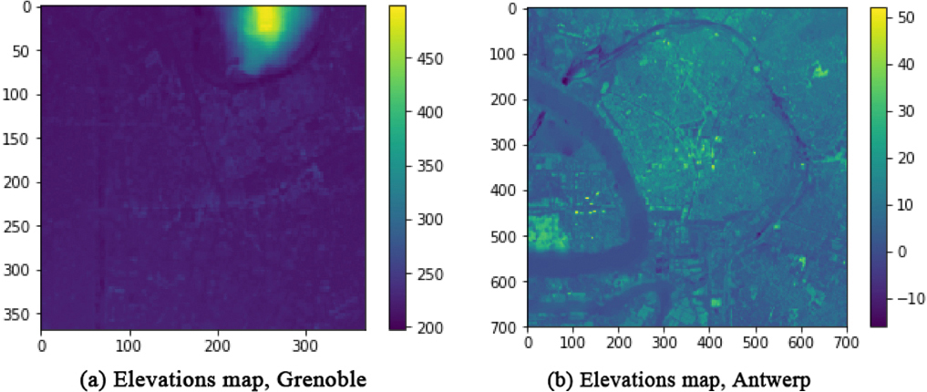

Our objective is to find the optimal architecture for UNet using these side-information and study the generalization ability of obtained models for RSSI map reconstruction.

As stated in Section 2.4, from the sets $(S^{j,i})_{\begin{subarray}{c}1\leqslant j\leqslant n\\ 1\leqslant i\leqslant m_{j}\end{subarray}}$ we use an evolutionary algorithm similar to [50] for searching the most efficient architecture represented as a Direct Acyclic Graph.3
³
https://colab.research.google.com/github/google-research/ google-research/blob/master/evolution/regularized_evolution_ algorithm/regularized_evolution.ipynb.

Here, the validation sets $(S^{j,i}_{v})_{\begin{subarray}{c}1\leqslant j\leqslant n\\ 1\leqslant i\leqslant m_{j}\end{subarray}}$ are put aside for hyperparameter tuning. The details for the Genetic algorithm are provided in Section 6.1. The edges of this acyclic graph represent data flow with only one input for each node, which is a single operation chosen among a set of candidate operations. We consider usual operations in the image processing field, that are a mixture of convolutional and pooling layers. We also consider three variants of 2D convolutional layers with kernels of size 3, 5 and 7, and two types of pooling layers that compute either the mean or the maximum on the filter of size 4.

Candidate architectures are built from randomly selected operations and the corresponding NN models are trained over the set $(S^{j,i}_{\ell})_{\begin{subarray}{c}1\leqslant j\leqslant n\\ 1\leqslant i\leqslant m_{j}\end{subarray}}$ and its (possible) combinations with side information. The resulted architectures are then ranked according to pixel-wise error between the interpolated result of the outputs over $(S^{j,i}_{v})_{\begin{subarray}{c}1\leqslant j\leqslant n\\ 1\leqslant i\leqslant m_{j}\end{subarray}}$ and interpolated measurements given by RBF interpolation by filtering out the buildings. As error functions, we have considered the Mean Absolute Error (MAE) or its Normalized version (NMAE) where we additionally weight the pixel error according to the distance matrix value. Best ranked model is then selected for mutation and placed in the trained population. The oldest and worst in the rank are then removed to keep the population size equal to 20 models.

The entire learning process is outlined in Algorithm 1. We begin with a labeled training dataset and utilize the RBF interpolation method to estimate measurements for unlabeled training data. The true measurements from the labeled training set and the RBF-estimated measurements are subsequently partitioned into smaller matrices, which are used as inputs to the NAS module. Once the NAS module identifies the neural network model with optimized architecture, $f_{\theta}$ , we address two scenarios for learning its associated parameters $\theta$ by minimizing the following objective function:

$\displaystyle\mathcal{L}(f_{\theta},S_{\ell}\cup S^{j,i}_{u\!\!\!\backslash})=% \frac{1}{n}\sum_{j=1}^{n}\frac{1}{m_{j}}\sum_{i=1}^{m_{j}}$ $\displaystyle\quad\left[\frac{1}{|S^{i,j}_{\ell}|}\!\!\sum_{(x,y)\in S^{i,j}_{% \ell}}\!\!\!\!\ell(y,f_{\theta}(x))\right.$ $\displaystyle\quad\left.+\frac{1}{|S^{j,i}_{u\!\!\!\backslash}|}\sum_{(x,% \tilde{y})\in S^{j,i}_{u\!\!\!\backslash}}\ell(\tilde{y},f_{\theta}(x))\right].$ (4)

These two scenarios relate to obtaining model parameters on labeled and pseudo-labeled measurements using just RBF interpolated data (scenario 1) or predictions from a first model learnt on these data (scenario 2).

Algorithm – 1. SL_NAS ^ind

Input: A labeled training set with given measurements: $(X^{j}_{m},Y^{j}_{m})_{1\leqslant j\leqslant n}$ and an unlabeled set $(X_{u}^{j})_{1\leqslant j\leqslant n}$

Init: Using $(X^{j}_{m},Y^{j}_{m})_{1\leqslant j\leqslant n}$ , find interpolated measurements $(\tilde{Y}^{j}_{u})_{1\leqslant j\leqslant n}$ over $(X_{u}^{j})_{1\leqslant j\leqslant n}$ using the RBF interpolation method;

Step 1: Cut the initial measurements maps $(Y_{m}^{j}\oplus\tilde{Y}^{j}_{u})_{1\leqslant j\leqslant n}$ into smaller matrices: $(S^{j,i})_{\begin{subarray}{c}1\leqslant j\leqslant n\\ 1\leqslant i\leqslant m_{j}\end{subarray}}$ . Step 2: Search the optimal NN architecture using $(S^{j,i})_{\begin{subarray}{c}1\leqslant j\leqslant n\\ 1\leqslant i\leqslant m_{j}\end{subarray}}$ ;

Scenario 1: Find the parameters $\theta^{\star}_{1}$ of the NN model $f_{\theta}$ :
$\displaystyle\theta^{\star_{1}}=\text{argmin}_{\theta}\mathcal{L}\left(f_{% \theta},S_{\ell}\cup S^{j,i}_{u\!\!\!\backslash}\right);$ (5) Scenario 2: Apply $f_{\theta^{\star}_{1}}$ on unlabeled data and obtain new pseudo-labeled measurements $S^{j,i}_{u\!\!\!\backslash}$ and find the new parameters $\theta^{\star}_{2}$ of the NN model $f_{\theta}$ :
$\displaystyle\theta^{\star_{2}}=\text{argmin}_{\theta}\mathcal{L}\left(f_{% \theta},S_{\ell}\cup S^{j,i}_{u\!\!\!\backslash}\right)$
Output: $f_{\theta^{\star}_{1}}$ for scenario 1 or $f_{\theta^{\star}_{2}}$ for scenario 2.

5. Evaluation setup

Algorithm – 1. SL_NAS ^ind
Input: A labeled training set with given measurements: $(X^{j}_{m},Y^{j}_{m})_{1\leqslant j\leqslant n}$ and an unlabeled set $(X_{u}^{j})_{1\leqslant j\leqslant n}$
Init: Using $(X^{j}_{m},Y^{j}_{m})_{1\leqslant j\leqslant n}$ , find interpolated measurements $(\tilde{Y}^{j}_{u})_{1\leqslant j\leqslant n}$ over $(X_{u}^{j})_{1\leqslant j\leqslant n}$ using the RBF interpolation method;
Step 1: Cut the initial measurements maps $(Y_{m}^{j}\oplus\tilde{Y}^{j}_{u})_{1\leqslant j\leqslant n}$ into smaller matrices: $(S^{j,i})_{\begin{subarray}{c}1\leqslant j\leqslant n\\ 1\leqslant i\leqslant m_{j}\end{subarray}}$ . Step 2: Search the optimal NN architecture using $(S^{j,i})_{\begin{subarray}{c}1\leqslant j\leqslant n\\ 1\leqslant i\leqslant m_{j}\end{subarray}}$ ;
Scenario 1: Find the parameters $\theta^{\star}_{1}$ of the NN model $f_{\theta}$ : $\displaystyle\theta^{\star_{1}}=\text{argmin}_{\theta}\mathcal{L}\left(f_{% \theta},S_{\ell}\cup S^{j,i}_{u\!\!\!\backslash}\right);$ (5) Scenario 2: Apply $f_{\theta^{\star}_{1}}$ on unlabeled data and obtain new pseudo-labeled measurements $S^{j,i}_{u\!\!\!\backslash}$ and find the new parameters $\theta^{\star}_{2}$ of the NN model $f_{\theta}$ : $\displaystyle\theta^{\star_{2}}=\text{argmin}_{\theta}\mathcal{L}\left(f_{% \theta},S_{\ell}\cup S^{j,i}_{u\!\!\!\backslash}\right)$ Output: $f_{\theta^{\star}_{1}}$ for scenario 1 or $f_{\theta^{\star}_{2}}$ for scenario 2.

We have considered three case studies from Paris, Antwerp (The Netherlands) and Grenoble. In the area of data-based research and in the field of machine learning singularly, it is usually hard to find large open-source datasets made of real data. In some works, however alternatively (or as a complement) to using real data, synthetic data can be generated, for instance through deterministic simulations.

In our study, we make use of three distinct databases of outdoor RSS measurements with respect to multiple base stations. The first one was generated through a Ray-Tracing tool in the city of Paris, France. The second database, which is publicly available (See [60]), consist of real GPS-tagged Long Range Wide Area Network (LoRaWAN) measurements that were collected in the city of Antwerp (The Netherlands). Finally, a third database, which is also made of real GPS-tagged LoRaWAN measurements, was specifically generated in the city of Grenoble (France), in the context of this study.

5.1 Paris dataset

This first dataset is made of synthetic outdoor RSS measurements, which were simulated in a urban Long Term Evolution (LTE) cellular context with a ray-tracing propagation tool named VOLCANO (commercialized by SIRADEL). Those simulations were calibrated by means of side field measurements [11]. This kind of deterministic tool makes use of both the deployment information (typically, the relative positions of mobile nodes and base stations) and the description of the physical environment (i.e., a city layout with a faceted description of the buildings, along with their constituting materials) to predict explicitly the electromagnetic interactions of the multipath radio signal between a transmitter and a receiver. Beyond the main limitations already mentioned in Section 2.1 regarding mostly computational complexity and prior information, we acknowledge a certain number of discrepancies or mismatches in comparison with the two other datasets based on real measurements. For example, in the simulated scenario, the dynamic range of observed RSS is continuous in the interval [ $-$ 190, $-$ 60] decibel-milliwatts (dBm), while with the real measurement data, a receiver sensitivity floor of $-$ 120 dBm is imposed. Moreover, the available simulation data was already pre-aggregated into cells. The overall scene is 1000 m $\times$ 1000 m, each pixel being 2 m $\times$ 2 m, thus forming a matrix of size 500 $\times$ 500. The area considered in these simulations is located in Paris between Champ de Mars (South-West), Faubourg Saint Germain (South), Invalides (Est), and Quai Branly / d’Orsay (North), as shown in Fig. 3.

Figure 3.

Buildings map and corresponding Base Stations positions (in red) for Paris dataset. The x and y axes are in meters.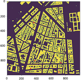

Figure 4.

Example of signal strength distribution (in dBm) generated through Ray-Tracing in the Paris dataset, with respect to one particular base station roughly located in (300 m, 300 m). The x and y axes are in meters.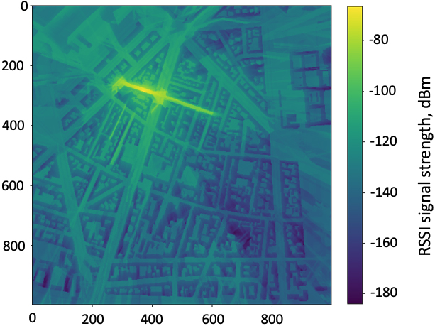

For each pixel, the RSS value was simulated with respect to 6 different Base Stations. An example is given for one of these base stations in Fig. 4. Further details regarding the considered simulation settings can be found in [11].

5.2 Antwerp dataset

Measurement campaign and experimental settings: The LoRaWAN dataset was collected in the urban are at the city centre of Antwerp from 17 November 2017 until 5 February 2018 [60, 61]. The dataset consists of 123,529 LoRaWAN messages with GPS coordinates on the map with RSSI measurements for that location. It was collected over a network driven by Proximus (which is a nation-wide network) by twenty postal service cars equipped with The City of Things hardware. The latitude, longitude and Horizontal Dilution of Precision information were obtained by the Firefly X1 GPS receiver and then sent in a LoRaWAN message by the IM880B-L radio module in the 868 MHz band. The interval between adjacent messages was from 30 s to 5 min depending on the Spreading Factor used.

The information was collected for 68 detected base stations in the initial database. We have filtered out some stations which have overall less than 10000 messages and/or which were located far from the collection zone having a flat signal. Finally we considered 9 base station – from Base-Station $\textit{BS}^{\prime}_{1}$ to Base-Station $\textit{BS}^{\prime}_{9}$ (see Fig. 5).

The initial dataset with information about each Base-Station (BS) or gateway (GW), Receiving time of the message (RX time), Spreading Factor, Horizontal Dilution of Precision, Latitude, Longitude looks as following.

Dataset preprocessing and analysis: As an example, in this part we will explain the way the dataset was processed for the future application. We aggregated the received power into cells of the size 10 meters $\times$ 10 meters (10 m $\times$ 10 m) and then averaged this power and translated into signal strength. To perform this aggregation, we measured the distance from the base station location based on local East, North, Up coordinates.

To compute the measurements density after data aggregation into cells of size 10 m $\times$ 10 m, we considered the close zone around the base station location of the size 3680 m $\times$ 3680 m. As an example, in the following Table 1 there is information about the first three considered base stations from this dataset.

Table 1
Amount of measurements for each base station located in the center of 368 $\times$ 368 image size after 10 m $\times$ 10 m aggregation, Antwerp dataset. Base stations with the highest amount of measurement points around the base station location were selected

Base station number	Amount of measurements after aggregation	Spatial density (per km²)
$BS^{\prime}_{1}$	6450	440
$BS^{\prime}_{2}$	5969	389
$BS^{\prime}_{3}$	7118	525

Figure 5.

Buildings map and corresponding considered 9 Base Stations positions (in red) for Antwerp dataset. The 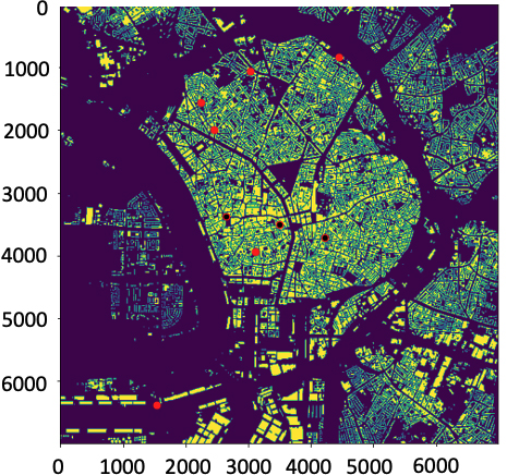$x$ and $y$ axes are in meters.

We consider the zone of full city of the size 7000 m $\times$ 7000 m which covers the positions and most of the collected measurements in the city area, and we did the 10 m $\times$ 10 m aggregation.

In the initial dataset if in the visited point on the map there was no captured signal, this point for corresponding base station was marked as $-$ 200 dBm, so in the Fig. 6 the informative range of the signal values lies in [ $-$ 120; $-$ 60] dBm, where the left boundary correspond to the sensitivity of the device.

Figure 6.

RSSI values distribution, base station Antwerp, 10 m 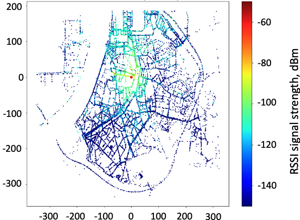$\times$ 10 m pixel resolution. The $x$ and $y$ axes are in meters.

5.3 Grenoble dataset

We have carried out an experimental campaign, and which is currently ongoing, aimed at gathering LoRA measurements within the actual urban setting of Grenoble city. This dataset holds significant value for future applications, primarily due to the scarcity of available data for research purposes in this domain. Furthermore, efforts are underway to expand this dataset further, which includes the installation of additional base stations and the collection of a larger volume of measurements, among other enhancements.

Just like for the Antwerp dataset, after removing outliers/artefacts, we then aggregated the signal in the cells. We converted the RSS into milliWatts (as dBm $=$ 10 $\log_{10}$ [mW]), computed its mean per cell in the cells of size 10 m $\times$ 10 m, and converted back the result into signal strength values. To perform this aggregation, we measured the distance from the base station $\textit{BS}_{1}$ location considered to be (0,0) 2D Cartesian coordinate based on local East, North, Up coordinates. Finally, we considered an overall area of interest of 3680 m $\times$ 3680 m (also for the radio mapping application), which covers the entire city, while containing most of the deployed base stations, as shown in Fig. 7.

To compare the measurements $s t d$ values per cell in different conditions, we considered two types of aggregation cell sizes: 50 m $\times$ 50 m and 10 m $\times$ 10 m, as shown in Fig. 8. In case of 50 m $\times$ 50 m aggregation cells, the amount of informative pixels (i.e., visited pixels with sufficient measurements) obviously reduces, but at the same time the aggregated value is more stable as a function of space (from pixels to pixels), while with 10 m $\times$ 10 m aggregation cells, we can see significantly larger fluctuations of the mean received power as a function of space but making available a larger amount of informative points for mapping.

The amount of measurements for two base stations in the Grenoble-1 dataset for 10 m $\times$ 10 m aggregation cells are shown in Table 2.

Table 2
Amount of measurements for 2 base stations in the Grenoble-1 dataset (first version). Only the Base stations with the highest amount of points were selected

Base station number	Amount of measurements after aggregation	Spatial density (per km²)
$\textit{BS}_{1}$	16577	1231
$\textit{BS}_{2}$	7078	515

Figure 7.

Part of the Grenoble map, with a selection of the deployed base station positions (red circles) and two canonical streets in LoS (red rectangles. The 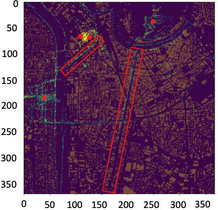$x$ and $y$ axes are in meters.

Figure 8.

RSSI values distribution, base station 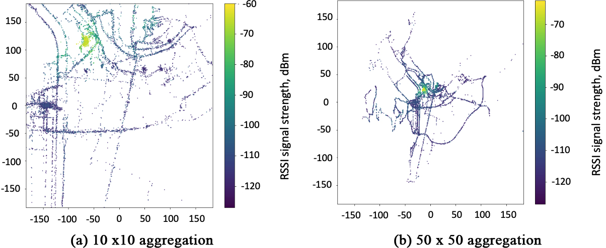$\textit{BS}_{1}$ Grenoble, for different aggregation cell sizes. The x and y axes are in meters.

Finally, the size of maps are 500 $\times$ 500 pixels for the generated dataset from Paris, 700 $\times$ 700 pixels for the dataset collected in Antwerp and 368 $\times$ 368 for Grenoble. For that, as a reminder, we aggregated and averaged the power of collected measurements in cells/pixels of size 10 meters $\times$ 10 meters by the measured distance from base station location based on local ENU coordinates for Grenoble and Antwerp, while for Paris dataset the cell size is 2 meters $\times$ 2 meters. As we also consider the generalization task, the algorithm should learn from all the available base stations data simultaneously.

In our settings, our available base station data is limited in scale, falling short by several orders of magnitude when compared to the datasets mentioned earlier. To address this inherent limitation, we devised a solution by artificially generating smaller submatrices from the original images by cutting them into smaller ones (we tested over 96 by 96 pixels size because of memory issues during learning of the neural network for the storing of the model weights). We also added the flipped and mirrored images and we also did a shift in 20 pixels meaning that in our dataset there were overlapping between the images. Moreover, if the amount of pixels with measurements in the initial cutted image was high enough (more than 3% of the presented pixels) then we masked out the randomly sampled rectangle of presented measurements similar to the cutout regularization ([62]). By doing this we force the algorithm to do the reconstructions in the zones without measurements (not only locally) and be more robust to the amount of input data.

Matrices of the side information were used in the models as additional channels concatenated with measurements map. Before feeding the data into the algorithm, all the values have been normalized between 0 and 1 in each channel separately before cutting them into smaller sizes to feed into the models.

Evaluation of the results over held out base stations: To evaluate the result we left one base station out of the initial set of each city to compare further the models performances with baselines, namely test Antwerp and test Grenoble. To do this, all the points were divided into two parts, namely train and test points for 90% and 10% respectively.

Figure 9.

Illustration of (a) Test points across various circular zones and (b) Training points within the corresponding region of the Antwerp dataset. The location of the base station is denoted by a black point. Coordinates are in meters.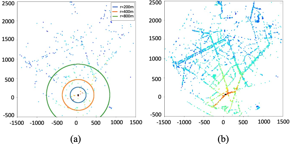

This will be used throughout all the following sections. Moreover, to highlight the importance of the zones close to base station (as it was mentioned in the Introduction) we compare the performance of the algorithms over different considered circles around the base station location, namely 200 meters, 400 meters and 800 meters radii (see Fig. 9).

Information about base stations for each city, amount of all points, points, that were used in the validation/test process, and training set are given in Table 4.

We considered state-of-the-art interpolation approaches which are: Total Variation (TV) in-painting by solving the optimization problem, Radial basis functions (RBF) [63] with linear kernel that was found the most efficient, and the $k$ Nearest Neighbors (kNN) regression algorithm. The evolutionary algorithm in the model search phase was implemented using the NAS-DIP[64] package.4

⁴

https://github.com/Pol22/NAS_DIP.

All experiments were run on NVIDIA GTX 1080 Ti 11GB GPU.

6. Experimental results

In our experiments, we are primarily interested in addressing the following two questions: $(a)$ does the use of side contextual information aid in the more accurate reconstruction of RSSI maps; and; $(b)$ to what extent is the search for an optimum NN design effective in the two scenarios considered (Section 4).

Regarding the first point, we consider the following learning settings:

1.
given only the measurements (no side information),
2.
given both measurements and distance maps,
3.
given measurements, distances and elevation maps,
4.
given measurements, distances maps and map of amount of buildings on the way from base station to corresponding point in the map (or, in other words, buildings count).

From the standpoint of application, accurate interpolation in all regions where the signal varies the most is critical. We will compare the cumulative mistakes across held-out pixels for each of the zones that are close enough to the test base station for the LoRa signal (by considering the fixed radius of 1 km).

In the following, we will present our findings using the UNet model utilizing side information as a multi-channel input.
6.1 Generalization ability of UNet

We conducted an architectural optimization search for UNet using a Genetic Algorithm similar to one presented in [19] with the implementation of [64]. To configure the genetic algorithm, we defined a mutation rate of 5% to encourage diversity within the population and promote convergence. Moreover, we permitted the encoder-decoder networks to have asymmetric structures. The population size was determined to be 20 individuals, and the number of generations for the algorithm to iterate through was set at 30. The architecture is characterized by its “U” shape, where the encoder down-samples the input image to capture features, and the decoder upsamples to generate the final output. The number of layers in each component of the obtained U-Net architecture varied depending on the dataset used. More specifically:

•
The encoder consists of multiple 2D-convolutional layers with Relu activation functions and having an increasing feature channels. The number of layers is determined based on experimentation and performance on the validation set. In our experiments, The convolutional layers found were 3 to 5 followed by a pooling or striding operation to reduce spatial dimensions. These configurations are fine-tuned after that the search of the architecture is completed.
•
The bridge found, was a stack of 5 to 7 2D-convolutional layers with a smaller receptive field. It is usually thinner in terms of feature channels compared to the encoder and decoder which prevents overfitting.
•
The decoder of the models contained also 3 to 5 layers, with transposed convolutions or up-sampling layers to increase spatial dimensions.
•
Skip connections were added between corresponding layers in the encoder and the decoder. There were as many skip connections as there were layers in the encoder and decoder.
•
Finally, the output layer which is responsible for generating the output RSSI sub-metric is a single convolutional layer with a sigmoid activation function. We have found that the fine-tuning part at the end produces meaningful predictions specific to the dataset.

It is to be noted that the number of layers is determined based on experimentation and performance on the validation set. Furthermore, to mitigate overfitting; dropout and batch normalization regularization techniques are incorporated during the optimization process. These methods introduce randomness during training, preventing the model from relying too heavily on specific features of the training set. As an example, Table 3 outlines the neural network architecture layers discovered during the architecture search phase for the RSSI Map of the city of Grenoble.

Table 3
Description of the Neural network architecture structure by layers found by the architecture search phase for the RSSI Map of the city of Grenoble used in our experiments

Layer Operation Input layer Size

1 (Conv2D+BatchNorm+LReLu) $\times$ 2+MaxPool (368,368,32)

1a Conv2D 1 (46,46,8)

1b SpaceToDepth+Conv2D 1 (184,184,64)

2 (Conv2D+BatchNorm+LReLu) $\times$ 2+MaxPool 1 (92,92,16)

2a DepthToSpace+Conv2D 2 (184,184,8)

3 (Conv2D+BatchNorm+LReLu) $\times$ 2+MaxPool 2 (92,92,8)

2a DepthToSpace+Conv2D 2 (184,184,8)

4 Concatenation 3+1b (46,46,16)

5 (Conv2D+BatchNorm+LReLu) $\times$ 2+Upsampling 4 (92,92,4)

6 Concatenation 5+3a (92,92,8)

7 (Conv2D+BatchNorm+LReLu) $\times$ 2+Upsampling 6 (184,184,8)

8 Concatenation 1a+2a+7 (184,184,80)

9 (Conv2D+BatchNorm+LReLu) $\times$ 2+Upsampling 8 (368,368,32)

10 (Conv2D+BatchNorm+LReLu) $\times$ 2 9 (368,368,32)

11 Conv2D 10 (368,368,1)

We first study the learnability of the UNet model for RSSI map reconstruction without the use of unlabeled data. In order to see if there is an effect of using side information we have just considered distance maps as additional context information and considered the model with a hand-crafted classical architecture used for in-painting [57]. The input was either only the measurements array or the measurements array stacked with the distances matrix.

The goal of this early experiment is to validate the usage of UNet for this task and investigate what effects the side information and labeled measurements have. For this we consider the simplest Paris data case where we keep only the points on the roads (as the points could be collected over the street by the vehicle drivers or pedestrians). The difference with Grenoble and Antwerp datasets is in the sampling procedure, as in reality it is very hard to obtain the collected data sampled uniformly in all the regions while in Paris dataset this is the case. All the RSSI measurements also exist in Paris dataset, this allows to see the importance of labeled information in the predictions by varying the percentage of labeled measurements in the training set.

Table 4
Summary over the settings for different cities: total amount of available measurements, points used as an input to the models, validation (test) points that were used also in the computation of the loss (during the evaluation)

City Name All points Train points Validation points Status

Grenoble $\textit{BS}_{1}$ 6264 5591 673 Train

$\textit{BS}_{2}$ 2728 2448 280 Train

$\textit{BS}_{3}$ 7266 6516 750 Train

$\textit{BS}_{4}$ 6836 6096 740 Test

Paris $\textit{BS}^{\prime\prime}_{1}-\textit{BS}^{\prime\prime}_{5}$ 250000 7495 242505 Train

$\textit{BS}^{\prime\prime}_{6}$ 250000 7495 242505 Test

Antwerp $\textit{BS}^{\prime}_{1}$ 6060 5440 620 Train

$\textit{BS}^{\prime}_{2}$ 5606 5034 572 Train

$\textit{BS}^{\prime}_{3}$ 7548 6785 763 Train

$\textit{BS}^{\prime}_{4}$ 2539 2276 263 Train

$\textit{BS}^{\prime}_{5}$ 2957 2667 290 Train

$\textit{BS}^{\prime}_{6}$ 4940 4453 487 Train

$\textit{BS}^{\prime}_{7}$ 3154 2829 325 Train

$\textit{BS}^{\prime}_{8}$ 8277 7455 822 Train

$\textit{BS}^{\prime}_{9}$ 4335 3888 447 Test

Figure 10 depicts the evolution of MAE in measurements with respect to the distance to the test base station getting lower in comparison with the RBF interpolation, as well as the overall error becomes smaller ( $\textit{BS}^{\prime\prime}_{6}$ – Table 4), of RBF, UNet using only measurements (UNet only msm) and UNet using measurements and distance maps (UNet msm+dist). From these results, it comes that RBF outperforms UNet using only measurements in a circle zone of less than 150 m radius around the base station. However, when distance maps are added to the model’s second channel, the situation is reversed.

Figure 10.
MAE for the distance from the base station for the RBF and fixed UNet outputs over Paris dataset with validation set compliment to the train one, measurements and distances or only measurements input.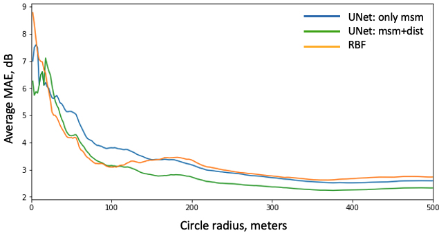

With the inclusion of side-information, we see that UNet performs around 1 point better in MAE than RBF. This situation is illustrated on the map reconstruction ability of both models around the test base station $\textit{BS}^{\prime\prime}_{6}$ in Fig. 11. As can be observed, the projected signal levels are more discernible on the roads, which are actually the zones of interest where the signal is sought, as predicted by the UNet model.

Figure 11.
Map reconstruction of RBF (left) and UNet (right) over the test base station 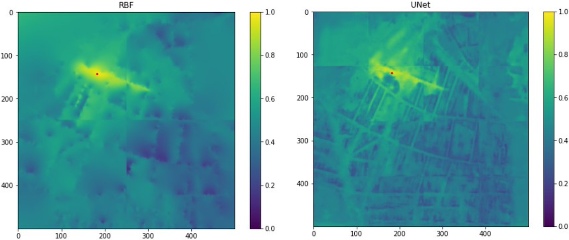$\textit{BS}^{\prime\prime}_{6}$ in Paris shown by a red dot.

As a result, these findings show that the UNet model can effectively account for side-information. We examined the RBF and UNet models for the influence of labeled measurements on the predictions by altering the percentage of labeled data utilized by RBF for discovering the interpolation and by the UNet model for learning the parameters. With regard to this proportion, Fig. 12 displays the average MAE 200 meters (left) and 400 meters (right) away from the test base station. The test error of the RBF model on unseen test data remains constant as the quantity of labeled training data increases, but the test error of the UNet model decreases as this number increases.

Figure 12.
MAE with respect to different percentage of labeled data in the training set 200 meters (left) and 400 meters (right) away from the test base station.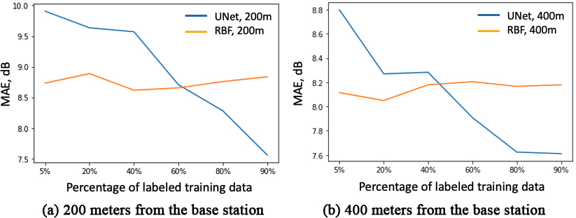

6.2 The use of unlabeled data by taking into account side information with NAS

City	Name	All points	Train points	Validation points	Status
Grenoble	$\textit{BS}_{1}$	6264	5591	673	Train
	$\textit{BS}_{2}$	2728	2448	280	Train
	$\textit{BS}_{3}$	7266	6516	750	Train
	$\textit{BS}_{4}$	6836	6096	740	Test
Paris	$\textit{BS}^{\prime\prime}_{1}-\textit{BS}^{\prime\prime}_{5}$	250000	7495	242505	Train
	$\textit{BS}^{\prime\prime}_{6}$	250000	7495	242505	Test
Antwerp	$\textit{BS}^{\prime}_{1}$	6060	5440	620	Train
	$\textit{BS}^{\prime}_{2}$	5606	5034	572	Train
	$\textit{BS}^{\prime}_{3}$	7548	6785	763	Train
	$\textit{BS}^{\prime}_{4}$	2539	2276	263	Train
	$\textit{BS}^{\prime}_{5}$	2957	2667	290	Train
	$\textit{BS}^{\prime}_{6}$	4940	4453	487	Train
	$\textit{BS}^{\prime}_{7}$	3154	2829	325	Train
	$\textit{BS}^{\prime}_{8}$	8277	7455	822	Train
	$\textit{BS}^{\prime}_{9}$	4335	3888	447	Test

We now expand our research to real-world data sets from Grenoble and Antwerp, taking into account more side-information and investigating the impact of neural architecture search on the creation of a better NN model. As in this case, the labeled training measurements are scarce we examine the usage of unlabeled data in addition to the labeled measurements as described in the previous section.

Table 5
Comparisons between baselines in terms of MAE with respect to the two distances to Antwerp’ test base station $\textit{BS}^{\prime}_{9}$ (left), and Grenoble test base station $\textit{BS}_{4}$ (right). Best results are shown in bold

Model	MAE, dB, 200 m	MAE, dB, 400 m
RBF[63]	8.34^↓	7.04^↓
kNN	7.98^↓	7.08^↓
TV	7.50^↓	6.97^↓
UNet[57]	6.37^↓	6.81^↓
DIP [65]	6.55^↓	6.63^↓
$f_{\theta^{\star}_{1}}$	5.88	6.37
RBF[63]	4.03^↓	5.29^↓
kNN	3.84^↓	4.92^↓
TV	4.53^↓	5.91^↓
DIP [65]	4.64^↓	5.50^↓
$f_{\theta^{\star}_{1}}$	3.40	4.32

We begin by envisaging scenario 1 of Algorithm 1 (Section 4) and investigating the impact of side information on the performance of the optimized NN model discovered by NAS.

Figure 13.

Cumulative MAE distribution of 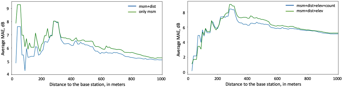$f_{\theta^{\star}_{1}}$ (scenario 1 of Algorithm 1) according to the distance to the test base station for the city of Antwerp $\textit{BS}^{\prime}_{9}$ ; with measurements and, measurements with distance maps (top) and measurements, distance maps, and elevation with and without building counts (down).

Figure 14.

Average MAE in dB of all models with respect to the distance to the test base Station 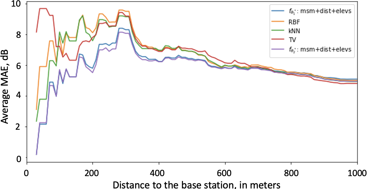$\textit{BS}^{\prime}_{9}$ for the city of Antwerp.

Figure 13 illustrates the evolution of MAE within a variable-radius circular zone for $f_{\theta^{\star}_{1}}$ trained solely on measurements and measurements accompanied by distance maps (upper panel). In contrast, the lower panel depicts the performance of $f_{\theta^{\star}_{1}}$ trained on measurements, distance maps, elevation, and building count for the test base stations of Antwerp $\textit{BS}^{\prime}_{9}$ . The integration of distance maps to complement measurements demonstrates enhanced prediction accuracy, consistent with our prior observations. When incorporating additional side information, such as building counts, the inclusion of elevation leads to superior signal estimations compared to scenarios where this information is omitted. This improvement can be attributed to the impact of building heights on signal transmission, highlighting the significance of considering elevation information in the training of the model.

As a best model obtained by Algorithm 1, scenario 1 we consider the case with three input channels: measurements, distances and elevations and present comparative results with other baselines in Table 5. The lowest errors are shown in boldface. The symbol ^↓ denotes that the error is significantly greater than the best result using the Wilcoxon rank sum test with a p-value threshold of 0.01. According to these findings, $f_{\theta^{\star}_{1}}$ outperforms other state-of-the-art models as well as the UNet model with a handcrafted architecture. These results suggest that the search of an optimal NN model with side-information has strong generalization ability for RSSI map reconstruction.

Figure 14 depicts the average MAE in dB of all models as well as the NN model $f_{\theta^{\star}_{2}}$ corresponding to scenario 2 of Algorithm 1, with respect to the distance to the test base Station $\textit{BS}^{\prime}_{9}$ for the city of Antwerp. For distances between 200 and 400 meters, $f_{\theta^{\star}_{2}}$ consistently outperforms in terms of MAE. As in paper [19], these findings imply that self-training constitutes a promising future direction for RSSI map reconstruction.

Figure 15 presents the average MAE in dB of all models with respect to the distance to the test base Station $\textit{BS}_{4}$ for the city of Grenoble. These results are consistent with those obtained over the city of Antwerp.

Figure 15.

Average MAE in dB of all models with respect to the distance to the test base Station 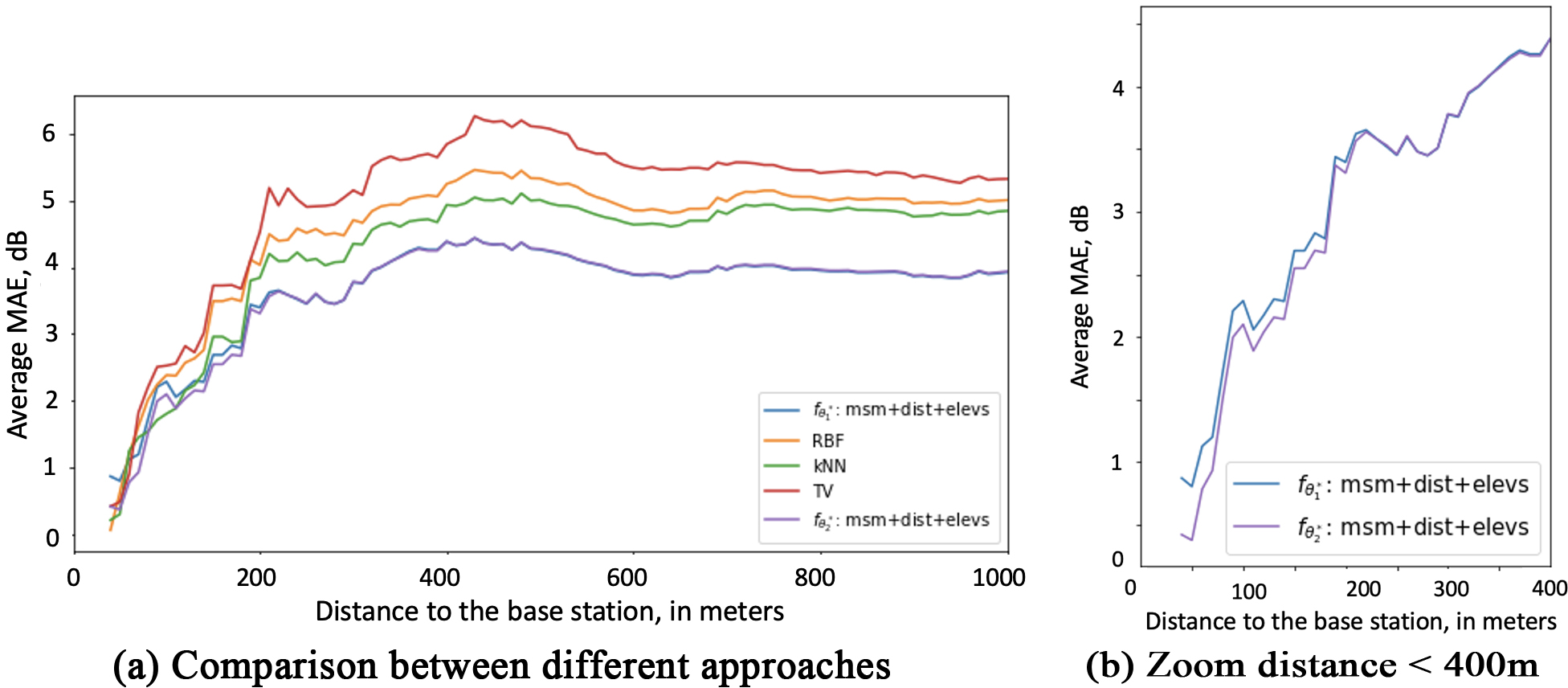$\textit{BS}_{4}$ for the city of Grenoble.

The general conclusion that we can draw is that knowing about local patterns (even if from different locations/distributions/base stations) allows us to use this information in signal strength map reconstruction for application to unseen measurements from different base stations, demonstrating the ability to generalize output in the same area. In order to get a finer granularity look at the estimations of the suggested technique, $f_{\theta^{\star}_{2}}$ , Fig. 16 depicts the errors heatmaps on circular zones of radius 200 m and 400 m surrounding the test base stations for Antwerp and Grenoble.

Figure 16.

Heatmap of the errors between true and predicted values of, 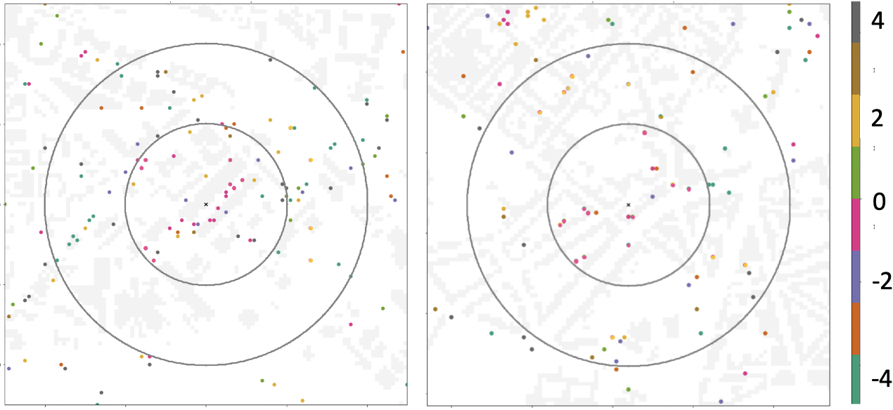$f_{\theta^{\star}_{2}}$ , over test base stations in Grenoble (left) and Antwerp (right).

Figure 17.

Empirical cumulative distribution function of different techniques in a 200-meter zone around the test base stations in Grenoble (left) and Antwerp (right).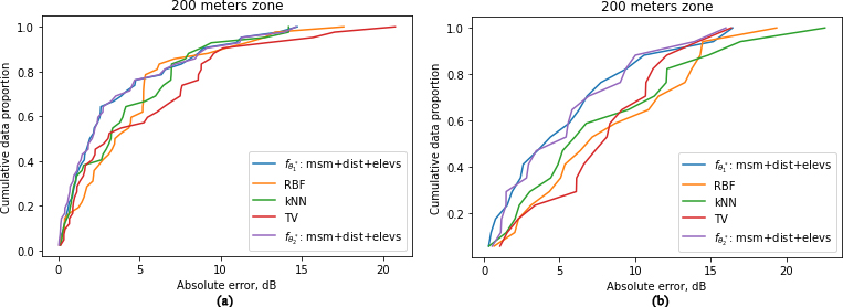

Figure 18.

MAE over the distance to the base station evaluated over unseen base stations for Grenoble (left) and Antwerp (right), 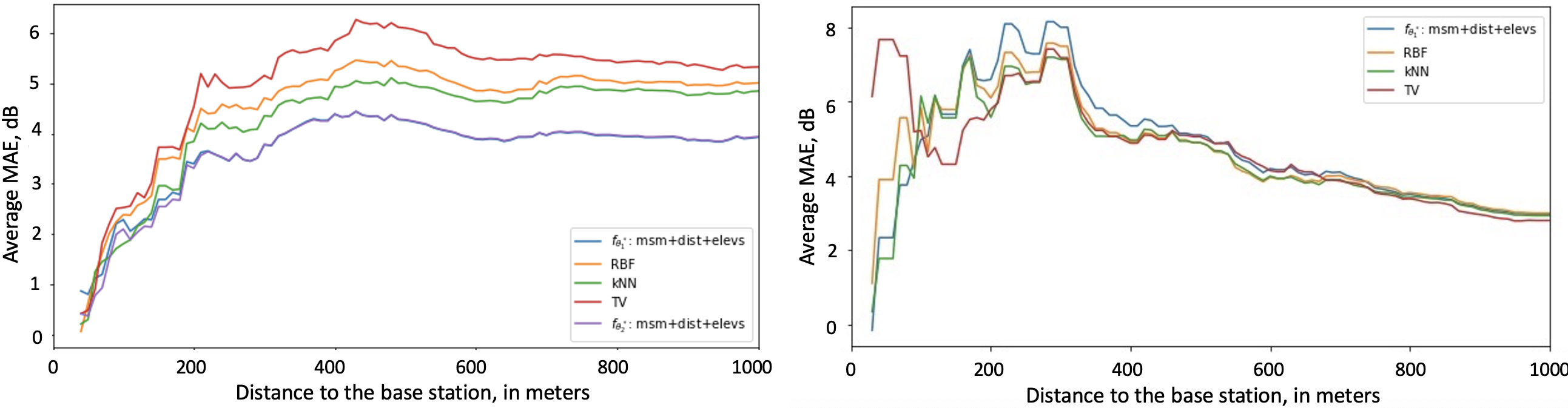$f_{\theta^{\star}_{1}}$ is trained over mixed dataset Grenoble+Antwerp.

Each point reflects the difference between the real and predicted signal values. For both cities, we notice that there is

•

an overestimation of the signal (higher predicted values than the true ones) within the zone of radius less than 200 meters where the values of the true signal are high. In absolute value, the average MAE in dB are respectively 3.6 for Grenoble and 6.3 for Antwerp.

•

an underestimation of the signal (lower predicted values than the true ones) within the zones of radius between 200 and 400 meters where the values of the true signal are low. In absolute value, the average MAE in dB are respectively 4.9 for Grenoble and 6.2 for Antwerp.

To better understand the aforementioned results, we provide the empirical cumulative distribution function of different techniques in a 200-meter zone around the test base stations in Grenoble (Fig. 17, left) and Antwerp (Fig. 17 right). From these results, it comes that the probabilities of having less absolute dB error is higher for both $f_{\theta^{\star}_{1}}$ and $f_{\theta^{\star}_{2}}$ than the other approaches.

The primary takeaway from these findings is that searching a Neural Network model with generalization capabilities might be useful for RSSI map reconstruction. To further investigate in this direction, we considered Scenario 1 of Algorithm 1 in which the training points of both cities are combined, with the goal of evaluating the model’s ability to produce predictions for one of the cities. The average MAE in db with respect to the distance to the base stations for different approaches are shown in Fig. 18.

Discussion: According to these findings, the inclusion of signal data from another city and the resulting disruption in the search for an efficient NN model for Received Signal Strength Indicator (RSSI) measurements highlight an important consideration in the field of machine learning for signal strength mapping. This disruption is primarily due to the fact that the characteristics of radio signal propagation can vary significantly from one location to another. The environmental conditions, infrastructure, and geographical layout all influence the behavior of radio waves.

Indeed, different locations have unique characteristics that affect radio signal propagation. For example, urban environments with tall buildings may exhibit different signal behaviors compared to rural areas with open landscapes. The presence of obstacles, building materials, and even weather conditions can impact signal strength. As a result, NN models trained on data from one location may not generalize well to another. When building NN models for RSSI measurements, it is essential to focus on their ability to generalize to new, unseen data. The disruption caused by incorporating data from a different city suggests that models need to adapt to the specific characteristics of the location they are deployed in. This is often referred to as “model adaptation”. It would be interesting to study over alignment strategies, such as those proposed for domain adaptation [66], in order to narrow the gap between these distributions in future work.

To address the challenges of location-specific characteristics, another approach is to develop an ensemble of models. Each model is trained on data from a specific location or under specific environmental conditions. The choice of which model to deploy can then be based on information about the incoming radio maps. For example, by using techniques like geolocation tagging to determine the source of the incoming data and selecting the corresponding model.

7. Conclusion and future work

In this paper, we conducted an extensive investigation into the importance of incorporating additional side information for optimizing NN architectures in the context of map reconstruction across three diverse datasets. Our research underscores the pivotal role that auxiliary data, such as building distance and elevation, can play in substantially enhancing the performance of NN models with tailored architectures. Specifically, we found that by augmenting our training data with these contextual features, we achieved a significant reduction in the mean absolute error in dB, affirming the efficacy of our optimized architecture.

Our proposed approach demonstrates a notable advantage over agnostic techniques, particularly in proximity to the test base stations. The model’s ability to accurately reconstruct signal strength maps, especially in the near vicinity of base stations, holds promising implications for practical applications such as urban planning and wireless network optimization. Importantly, our analysis reveals that our NN-based approach exhibits strong generalization capabilities, bolstering its utility in varying real-world scenarios.

However, it is essential to acknowledge that in situations where a distribution shift between two maps exists, the predictive confidence provided by the trained model may exhibit biases that render it less reliable. Substantial dissimilarities between two different Received Signal Strength Indicator (RSSI) maps can lead to a substantial degradation in the model’s performance due to inaccuracies in pseudo-labels. While techniques like noise modelling may mitigate some of these issues in practice [67], it is vital to note that there remains a theoretical gap in our understanding. Specifically, exploring semi-supervised learning techniques under distribution shifts represents an important avenue for future research.

To address this challenge effectively, future work could focus on the development of Neural Dynamic Classification algorithms that adapt dynamically to distribution shifts [68]. These algorithms would enable the model to update its pseudo-labeling strategy based on evolving data distributions, enhancing its robustness in the face of changing environments.

Furthermore, the incorporation of Dynamic Ensemble Learning Algorithms could be explored to combine predictions from multiple models, each specialized for different distribution scenarios [69]. This ensemble approach may help mitigate the impact of distribution shifts by selecting the most appropriate model for the given context, further improving the reliability and accuracy of map reconstructions.

Additionally, self-supervised learning techniques offer a promising direction for enhancing the model’s performance under distribution shifts [70]. By leveraging self-supervised learning, the model can learn useful representations from unlabeled data and adapt to new distribution patterns more effectively.

In summary, our findings underscore the potential of tailored NN architectures and the significance of auxiliary data in map reconstruction. However, addressing the challenges posed by distribution shifts remains an important direction for future research, with the potential for Neural Dynamic Classification algorithms, Dynamic Ensemble Learning Algorithms, and self-supervised learning to play a pivotal role in enhancing model reliability and accuracy in diverse and evolving scenarios.

References

Khelifi

Bradai

Benslimane

Rawat

Atri

. A Survey of Localization Systems in Internet of Things. Mobile Networks and Applications. 2019 Jun; 24(3): 761-785.

Sharp

Guo

. Ground-Based Wireless Positioning. John Wiley & Sons, Ltd; 2009.

Dargie

Poellabauer

. Fundamentals of Wireless Sensor Networks: Theory and Practice. John Wiley & Sons, 2010.

Cheng

Zhang

Maple

. A Survey of Localization in Wireless Sensor Network. International Journal of Distributed Sensor Networks. 2012; 12: 2012.

Choi

Chang

Jung

Song

. Low-Power LoRa Signal-Based Outdoor Positioning Using Fingerprint Algorithm. ISPRS International Journal of Geo-Information. 2018; 7(11).

Redondi

AEC

. Radio Map Interpolation Using Graph Signal Processing. IEEE Communications Letters. 2018; 22(1): 153-156.

Powell

MJD

. In: Radial Basis Functions for Multivariable Interpolation: A Review. USA: Clarendon Press; 1987, pp. 143-167.

Enrico

Redondi

. Radio Map Interpolation Using Graph Signal Processing. IEEE Communications Letters. 2018; 22(1): 153-156.

Oliver

Webster

. Kriging: a method of interpolation for geographical information systems. International Journal of Geographical Information System. 1990; 4(3): 313-332.

10.

Liao

Sun

Wang

. Radio Environment Map Construction by Kriging Algorithm Based on Mobile Crowd Sensing. Wireless Communications and Mobile Computing. 2019 02; 2019: 1-12.

11.

Brau

Corre

Lostanlen

. Assessment of 3D network coverage performance from dense small-cell LTE. In: IEEE International Conference on Communications (ICC); 2012; pp. 6820-6824.

12.

Laaraiedh

Uguen

Stephan

Corre

Lostanlen

Raspopoulos

, et al. Ray tracing-based radio propagation modeling for indoor localization purposes. In: 2012 IEEE 17th International Workshop on Computer Aided Modeling and Design of Communication Links and Networks (CAMAD); 2012. pp. 276-280.

13.

Raspopoulos

, et al. Cross device fingerprint-based positioning using 3D Ray Tracing. In: Proc. % International Wireless Communications and Mobile Computing Conference IWCMC’12; 2012. pp. 147-152.

14.

Sorour

Lostanlen

Valaee

Majeed

. Joint Indoor Localization and Radio Map Construction with Limited Deployment Load. IEEE Transactions on Mobile Computing. 2015; 14(5): 1031-1043.

15.

Levie

Yapar

Kutyniok

Caire

. Pathloss Prediction using Deep Learning with Applications to Cellular Optimization and Efficient D2D Link Scheduling. In: ICASSP, 2020; pp. 8678-8682.

16.

Hayashi

Nagao

Ito

. A study on the variety and size of input data for radio propagation prediction using a deep neural network. In: 14th European Conference on Antennas and Propagation (EuCAP); 2020. pp. 1-5.

17.

Nagao

Hayashi

. Study on radio propagation prediction by machine learning using urban structure maps. In: 14th European Conference on Antennas and Propagation (EuCAP); 2020. pp. 1-5.

18.

Elsken

Metzen

Hutter

. Neural Architecture Search: A Survey. Journal of Machine Learning Research. 2019; 20(55): 1-21. Available from: http//jmlr.org/papers/v20/18-598.html.

19.

Malkova

Pauletto

Villien

Denis

Amini

. Self-Learning for Received Signal Strength Map Reconstruction with Neural Architecture Search. In: 31 International Conference on Artificial Neural Networks; 2022. pp. 515-526.

20.

Malkova

Amini

Denis

Villien

. Radio Map Reconstruction with Deep Neural Networks in a Weakly Labeled Learning Context with use of Heterogeneous Side Information. In: 4th International Conference on Advances in Signal Processing and Artificial Intelligence; 2022.

21.

Heap

. A review of comparative studies of spatial interpolation methods in environmental sciences: Performance and impact factors. Ecological Informatics. 2011; 6(3): 228-241.

22.

Rusu

. Radial Basis Functions Versus Geostatistics in Spatial Interpolations. In: International Federation for Information Processing Digital Library; Artificial Intelligence in Theory and Practice. vol. 217; 2006.

23.

Fan

Xiang

Puthal

Gong

Nanda

, et al. Towards System Implementation and Data Analysis for Crowdsensing Based Outdoor RSS Maps. IEEE Access. 2018; 6: 47535-47545.

24.

Kubota

Tagashira

Arakawa

Kitasuka

Fukuda

. Efficient Survey Database Construction Using Location Fingerprinting Interpolation. In: 2013 IEEE 27th International Conference on Advanced Information Networking and Applications (AINA); 2013. pp. 469-476.

25.

Ning

, et al. Outdoor Location Estimation Using Received Signal Strength-Based Fingerprinting. Wireless Pers Commun. 2016; 99: 365-84.

26.

Lin

Dong

Gao

. SateLoc: A Virtual Fingerprinting Approach to Outdoor LoRa Localization using Satellite Images. In: 19th ACM/IEEE International Conference on Information Processing in Sensor Networks (IPSN); 2020. pp. 13-24.

27.

Raspopoulos

Laoudias

Kanaris

Kokkinis

Panayiotou

Stavrou

. 3D Ray Tracing for device-independent fingerprint-based positioning in WLANs. In: 2012 9th Workshop on Positioning, Navigation and Communication; 2012. pp. 109-113.

28.

Sorour

, et al. RSS Based Indoor Localization with Limited Deployment Load. In: Proc. IEEE Global Communications Conference (GLOBECOM’12); 2012. pp. 303-308.

29.

Ronneberger

Fischer

Brox

. U-Net: Convolutional Networks for Biomedical Image Segmentation. In: Medical Image Computing and Computer-Assisted Intervention (MICCAI). vol. 9351 of LNCS. Springer; 2015. pp. 234-241.

30.

Han

Xue

Liu

. A Two-Phase Transfer Learning-Based Power Spectrum Maps Reconstruction Algorithm for Underlay Cognitive Radio Networks. IEEE Access. 2020; 8: 81232-81245.

31.

Sato

Inage

Fujii

. On the Performance of Neural Network Residual Kriging in Radio Environment Mapping. IEEE Access. 2019; 7: 94557-94568.

32.

Zhu

Cheng

Zhang

Yao

Gao

Liu

. Spatial interpolation using conditional generative adversarial neural networks. International Journal of Geographical Information Science. 2020; 34(4): 735-758.

33.

Yin

Pajot

Bézenac

Gallinari

. Unsupervised Inpainting for Occluded Sea Surface Temperature Sequences. In: Proceedings of the 9th International Workshop on Climate Informatics (CI). Paris, France; 2019. Available from: https//drive.google.com/drive/folders/1-59qXM-hzPSPkbn_51rcnDjaaIw7XeQJ.

34.

Inoue

Ichige

Nagao

Hayashi

. Radio Propagation Prediction Using Deep Neural Network and Building Occupancy Estimation. 2020 International Symposium on Antennas and Propagation (ISAP). 2021; pp. 315-316.

35.

Chapelle

Schölkopf

Zien

, editors. Semi-Supervised Learning. The MIT Press, 2006.

36.

Seeger

. Learning with Labeled and Unlabeled Data. University of Edinburgh, 2001.

37.

Basu

Banerjee

Mooney

. Semi-supervised Clustering by Seeding. In: Proceedings of the Nineteenth International Conference on Machine Learning; 2002; pp. 27-34.

38.

Maximov

Amini

Harchaoui

. Rademacher Complexity Bounds for a Penalized Multi-class Semi-supervised Algorithm. J Artif Intell Res. 2018; 61: 761-786.

39.

Zhang

Oles

. A probability analysis on the value of unlabeled data for classification problems. In: 17th International Conference on Machine Learning; 2000.

40.

Belkin

Niyogi

. Semi-Supervised Learning on Riemannian Manifolds. Machine Learning. 2004; 56(1-3): 209-239.

41.

Cohen

Cozman

Sebe

Cirelo

Huang

. Semisupervised Learning of Classifiers: Theory, Algorithms, and Their Application to Human-Computer Interaction. IEEE Transactions on Pattern Analysis and Machine Intelligence. 2004; 26(12): 1553-1567.

42.

Amini

Laviolette

Usunier

. A Transductive Bound for the Voted Classifier with an Application to Semi-supervised Learning. In: Advances in Neural Information Processing Systems (NeurIPS 21); 2008. pp. 65-72.

43.

Feofanov

Devijver

Amini

. Transductive Bounds for the Multi-Class Majority Vote Classifier. In: The Thirty-Third AAAI Conference on Artificial Intelligence; 2019; pp. 3566-3573.

44.

Krithara

Amini

Renders

Goutte

. Semi-Supervised Document Classification with a Mislabeling Error Model. In: 30th European Conference on Information Retrieval. Glasgow; 2008. pp. 370-381.

45.

Amini

Feofanov

Pauletto

Hadjadj

Devijver

Maximov

. Self-Training: A Survey. CoRR. 2022abs/ 2202.12040.

46.

Xue

Zhang

Neri

. A Method based on Evolutionary Algorithms and Channel Attention Mechanism to Enhance Cycle Generative Adversarial Network Performance for Image Translation. Int J Neural Syst. 2023; 33(5): 23500261-2350026:15.

47.

Urdiales

Martín

Armingol

. An improved deep learning architecture for multi-object tracking systems. Integr Comput Aided Eng. 2023; 30(2): 121-134.

48.

Ding

Nie

Liu

Wang

Yuan

. Compact Convolutional Neural Network with Multi-Headed Attention Mechanism for Seizure Prediction. Int J Neural Syst. 2023; 33(3): 23500141-2350014:18.

49.

Zoph

. Neural architecture search with reinforcement learning. arXiv preprint arXiv161101578. 2016.

50.

Real

Aggarwal

Huang

. Regularized evolution for image classifier architecture search. In: AAAI. vol. 33; 2019. pp. 4780-4789.

51.

Jin

Song

. Auto-keras: An efficient neural architecture search system. In: Proceedings of the 25th ACM SIGKDD; 2019. pp. 1946-1956.

52.

Liu

Simonyan

Yang

. Darts: Differentiable architecture search. In: International Conference on Learning Representations; 2019.

53.

Liu

Chen

Schroff

Adam

Hua

Yuille

, et al. Auto-deeplab: Hierarchical neural architecture search for semantic image segmentation. In: Proceedings of CVPR; 2019; pp. 82-92.

54.

Song

Chen

Zhang

Wang

, et al. Learning Dynamic Routing for Semantic Segmentation; 2020.

55.

Zhang

Wang

Wei

Liu

. An Efficient Multi-Objective Evolutionary Zero-Shot Neural Architecture Search Framework for Image Classification. Int J Neural Syst. 2023; 33(5): 2350016:1–2350016:15. Available from: doi: 10.1142/S0129065723500168.

56.

Xue

Jiang

Neri

Liang

. A Multi-Objective Evolutionary Approach Based on Graph-in-Graph for Neural Architecture Search of Convolutional Neural Networks. Int J Neural Syst. 2021; 31(9): 1-17.

57.

Ronneberger

Fischer

Brox

. U-net: Convolutional networks for biomedical image segmentation. In: International Conference on Medical image computing and computer-assisted intervention; 2015; pp. 234-241.

58.

Boeing

. OSMnx: A Python package to work with graph-theoretic OpenStreetMap street networks. Journal of Open Source Software. 2017; 2(12): 215.

59.

Rappaport

. Wireless communications: Principles and practice. Prentice Hall; 2002.

60.

Aernouts

Berkvens

Vlaenderen

Weyn

. Sigfox and LoRaWAN Datasets for Fingerprint Localization in Large Urban and Rural Areas. Data. 2018; 3(2).

61.

Aernouts

. Localization with low power wide area networks. University of Antwerp; 2022.

62.

Devries

Taylor

. Improved Regularization of Convolutional Neural Networks with Cutout. CoRR. 2017; abs/1708. 04552. Available from: http//arxiv.org/abs/1708.04552.

63.

Bishop

. Pattern Recognition and Machine Learning (Information Science and Statistics). Berlin, Heidelberg: Springer-Verlag; 2006.

64.

Gilbert

Jin

Collomosse

. Neural Architecture Search for Deep Image Prior. Computers and Graphics. 202198.

65.

Ulyanov

Vedaldi

Lempitsky

. Deep Image Prior. In: IEEE Conference on Computer Vision and Pattern Recognition; 2018; pp. 9446-9454.

66.

k Kumar

Sattigeri

Wadhawan

Karlinsky

Feris

Freeman

, et al. Co-regularized Alignment for Unsupervised Domain Adaptation. In: Advances in Neural Information Processing Systems (NeurIPS 32); 2018. pp. 9367-9378.

67.

Hadjadj

Amini

Louhichi

. Generalization Guarantees of Self-Training of Halfspaces under Label Noise Corruption. In: Proceedings of the Thirty-Second International Joint Conference on Artificial Intelligence, IJCAI-23; 2023. pp. 3777-3785. Main Track. Available from: doi: 10.24963/ijcai.2023/420.

68.

Rafiei

Adeli

. A New Neural Dynamic Classification Algorithm. IEEE Transactions on Neural Networks and Learning Systems. 2017; 28(12): 3074-3083.

69.

Pereira

Piteri

Souza

Papa

Adeli

. FEMa: A Finite Element Machine for Fast Learning. Neural Comput Appl. 2020; 32(10): 6393-6404.

70.

Rafiei

Gauthier

Adeli

Takabi

. Self-Supervised Learning for Electroencephalography. IEEE Transactions on Neural Networks and Learning Systems. 2022; pp. 1-15.

Layer	Operation	Input layer	Size
1	(Conv2D+BatchNorm+LReLu) $\times$ 2+MaxPool		(368,368,32)
1a	Conv2D	1	(46,46,8)
1b	SpaceToDepth+Conv2D	1	(184,184,64)
2	(Conv2D+BatchNorm+LReLu) $\times$ 2+MaxPool	1	(92,92,16)
2a	DepthToSpace+Conv2D	2	(184,184,8)
3	(Conv2D+BatchNorm+LReLu) $\times$ 2+MaxPool	2	(92,92,8)
2a	DepthToSpace+Conv2D	2	(184,184,8)
4	Concatenation	3+1b	(46,46,16)
5	(Conv2D+BatchNorm+LReLu) $\times$ 2+Upsampling	4	(92,92,4)
6	Concatenation	5+3a	(92,92,8)
7	(Conv2D+BatchNorm+LReLu) $\times$ 2+Upsampling	6	(184,184,8)
8	Concatenation	1a+2a+7	(184,184,80)
9	(Conv2D+BatchNorm+LReLu) $\times$ 2+Upsampling	8	(368,368,32)
10	(Conv2D+BatchNorm+LReLu) $\times$ 2	9	(368,368,32)
11	Conv2D	10	(368,368,1)

Neural architecture search for radio map reconstruction with partially labeled data

Abstract

Keywords

1. Introduction

1 https://sarws.eu/.

2.1 Interpolation and data-augmentation techniques

2.2 NN based models trained after data augmentation

2.3 Semi-supervised learning

2.4 Neural architecture search

3. Application to the stated RSS map reconstruction problem

5.1 Paris dataset

Table 1 Amount of measurements for each base station located in the center of 368 × 368 image size after 10 m × 10 m aggregation, Antwerp dataset. Base stations with the highest amount of measurement points around the base station location were selected

Table 2 Amount of measurements for 2 base stations in the Grenoble-1 dataset (first version). Only the Base stations with the highest amount of points were selected

Table 5 Comparisons between baselines in terms of MAE with respect to the two distances to Antwerp’ test base station 𝐵𝑆 9 ′ (left), and Grenoble test base station 𝐵𝑆 4 (right). Best results are shown in bold

References

¹
https://sarws.eu/.

Table 1
Amount of measurements for each base station located in the center of 368 $\times$ 368 image size after 10 m $\times$ 10 m aggregation, Antwerp dataset. Base stations with the highest amount of measurement points around the base station location were selected

Table 2
Amount of measurements for 2 base stations in the Grenoble-1 dataset (first version). Only the Base stations with the highest amount of points were selected

Table 5
Comparisons between baselines in terms of MAE with respect to the two distances to Antwerp’ test base station $\textit{BS}^{\prime}_{9}$ (left), and Grenoble test base station $\textit{BS}_{4}$ (right). Best results are shown in bold