Prediction of thrust bearing’s performance in Mixed Lubrication regime

Abstract

A hydrodynamic thrust bearing could be forced to operate in mixed lubrication regime under various circumstances. At this state, the tribological characteristics of the bearing could be affected significantly and the developed phenomena would have a severe impact on the performance of the mechanism. Until recently, researchers were modeling the hydrodynamic lubrication problem of the thrust bearings either with analytical or with numerical solutions. The analytical solutions are very simple and do not provide enough accuracy in describing the actual problem. To add to that, following only computational methodologies, can lead to time consuming and complex algorithms that need to be repeated every time the operating conditions change, in order to draw safe conclusions. Recent technological advances, especially on the field of computer science, have provided tools that enhance and accelerate the modeling of thrust bearings’ operation. The aim of this study is to examine the application of Artificial Neural Networks as Machine Learning models, that are trained to predict the coefficient of friction for lubricated pad thrust bearings in mixed lubrication regime. The hydrodynamic analysis of the thrust bearing is performed by solving the Average 2-D Reynolds equation numerically. In order to describe the roughness of the profiles, both the flow factors suggested by N. Patir and H.S. Cheng (1978) and the model of J.A. Greenwood and J. H. Tripp (1970) are taken into consideration. Three lubricants, the SAE 0W30, the SAE 10W40 and the SAE 10W60, are tested and compared for a variety of operating velocities and applied coatings. The numerical analysis results are used as training datasets for the machine learning algorithms. Four different ML methods are applied in this investigation: Artificial Neural Networks (ANNs), Multi- Variable Quadratic Polynomial Regression, Quadratic SVM and Regression Trees. The coefficient of determination, $R^{2}$ is calculated and used to determine the most accurate ML method for the current study. The results showed that ANNs provide very good accuracy in the prediction of friction coefficient compared to the rest of the ML models discussed.

Keywords

ANN thrust bearing mixed lubrication numerical analysis machine learning

1. Introduction

Thrust bearings are machine elements that were designed to carry the axial loads developed in rotating machinery. The lubricant that is dragged inside the tribo-conjunction due to the relative motion of the rotor and the pad, along with the wedge, between the two friction surfaces, constitute the basic principle of operation of such mechanisms. The design of thrust bearings has become demanding through time due to the environmental and economic limitations that call for cost efficient applications with compact sizes. The ability of these bearings to support axial loads in many operating conditions has turned them into crucial machine elements in industry, marine, aerospace and automotive fields. For example, Kalsi et al. [1] investigated a load-responsive hydrodynamic thrust bearing able to operate in higher load and speed than standard bearings, especially for downhole drilling tools. Furthermore, Lingwall et al. [2] investigated the application and qualification of PCD thrust bearings in the extreme conditions of marine hydrokinetic machines. To add to that, Sun et al. [3] investigated the application of rubber-supported thrust bearings in marine thrusters in a way to overcome the wear that appears in some of the pads when the load is not evenly distributed.

There are cases in which the bearings are forced to operate efficiently under extreme conditions which may lead to mixed or even boundary lubrication. Such cases must be understood, analyzed and included in the final bearings’ design, because the impact of the forces developed under these operating conditions may affect significantly the final performance of the bearing as well as the corresponding mechanism. To add to that, investigators have applied a variety of methods to enhance thrust bearings’ performance, focusing on their surface profiles, dimples, and textures as well as coatings [8, 9, 10, 11, 12, 13, 14, 15]. To begin with, Etsion et al. [4] worked on the improvement of thrust bearing’s performance by applying laser-surface texturing. Moreover, Knuteson et al. [5] investigated the wear-in behavior of PCD coatings on thrust bearings. In addition, Qi et al. [6] presented research results on the tribological behaviors of annular rings with spiral grooves. Finally, Zhang et al. [7] performed a numerical analysis and an experimental research on the load carrying capacity of water-lubricated tilting-pad thrust bearings.

From the early investigations it was clear that friction played an important role on the characteristics of the lubricated contacts and the operational regime of the corresponding mechanism. Three main lubrication regimes derive from the fraction of the film thickness and the average surface roughness: the hydrodynamic, the mixed and the boundary lubrication regime. Standard designs of thrust bearings, provide operation under hydrodynamic lubrication, where the roughness heights of the pads and the rotor are insignificant in comparison to the minimum film thickness; thus, there can be no contact amongst them. In this case only hydrodynamic conditions and loads affect the performance of the bearing. When the roughness of the mechanism is high enough, or when the lubricant’s thickness reduces at a level that a contact between asperities is possible, the thrust bearing may operate under mixed lubrication.

It is a fact that some thrust bearings are forced, or even designed, to operate under mixed lubrication. Extreme conditions of operation like very low sliding velocity or high external loads may lead to the appearance of contact areas between the asperities of the two friction surfaces. To add to that, transition faces like startup and shutdown, or sudden deviations from normal operation, may also cause periodic operation of the thrust bearing within mixed lubrication regime. During the years, many researches have approached the investigation of the mixed lubrication regime in thrust bearings’ operation both experimentally and analytically. First of all, Wang et al. [8] presented a study on water lubricated silicon carbide thrust bearings that were designed to operate between hydrodynamic and mixed lubrication regime, with a surface texture. The selected texture included micro-pits, distributed in a square area. The results showed that the bearing was able to carry almost double the load when the proper design of micro-pits was applied compared to the un-textured surface. Furthermore, Etsion [4] performed a theoretical and experimental study on the use of Laser Surface Texturing (LST) for various machine elements. LST was used in order to create micro-dimples on the components. The results showed that the micro-dimples assist the bearing’s operation, on the one hand, as micro-hydrodynamic bearings when the operation was within full hydrodynamic or mixed lubrication regime, or as a micro-reservoir, when starvation occurred, leading to substantial reduction of friction in comparison to the non-textured components. Moreover, Illner et al. [9] built a simulation program for a thrust bearing operating in a diesel injection pump. The algorithm was based on the numerical solution of the Reynolds equation for unsteady load, velocity and movement conditions. These conditions, combined to the low viscosity of the fuel, forced the bearing to operate under mixed lubrication with high solid body contact pressures. They concluded that convex slide faces do not produce significant improvements; however, they cause deterioration of the operating behavior. Finally, Henry et al. [10] investigated the behavior of many kinds of fixed-geometry thrust bearings in start-up condition and mixed lubrication. The study showed that there can be a texture design, appropriate to create a lubrication film that gives the bearing the ability to lift up during start-up. The results showed that the effect of squeezing was higher in start-up process than in shutdown. All in all, it can be seen that, various investigations have been performed focusing on improving the performance of thrust bearings in mixed lubrication regime by applying different surface profiles, textures, lubricants and coatings.

Current advances in computer science have led to improvements and applications in all engineering fields. For instance, Rodriguez-Galiano et al. [11] compared various machine learning algorithms in order to identify the optimum predictive model for mineral prospectivity. Furthermore, Fernandes et al. [12] investigated intelligent home management systems that perform power management, based on the user’s behavior in nearly real-time. Moreover, Li et al. [13] presented a case study regarding unmanned aerial vehicles landing on unmanned surface vehicles, proposing the application of cognitive twins as a way to enhance decision making. To add to that, Yun et al. [14] applied deep learning in order to improve the excessive computational time required for operational modal analysis of structures. In adition, Ruiz et al. [15] proposed a convolutional neural network in order to improve the autonomy of machinery included in aerospace manufacturing procedures. Finaly, Urdiales et al. [16] presented a multi-object tracking system, based on the Kalman filter, using a deep learning approach in order to improve autonomous driving in crowded urban roads. In the field of tribology, machine learning applications still constitute a new era of research [17], which is gradually expanding in every direction of the field. To begin with, Alves et al. [18] created a deep convolutional neural network, based on simulation data of ovalization fault conditions. The developed network was found to be accurate enough to predict the corresponding fault conditions. Furthermore, R. L. Lorza et al. [19, 20], investigated the use of FEM and data mining as combined methodologies to build a prediction model for tapered roller bearings, able to predict the maximum load carrying capacity of the mechanism. After building the FEM model of the bearing, a group of regression models was tested regarding the accuracy to predict the contact ration that appears on the bearing, for the applied loads. Moreover, Rossopoulos and Papadopoulos [21] investigated the performance of marine bearings by developing a machine learning-based analytics methodology. The machine learning algorithms were trained with data provided from a misaligned hydrodynamically lubricated journal bearing. Finally, Kokkinidis and Nikolakopoulos [22] studied the performance of misaligned journal bearings by training an Artificial Neural Network based on data from numerical simulations.

This paper extends the Machine Learning approach of [23] by adding one more method, Artificial Neural Networks (ANNs), in the authors’ effort to combine numerical and machine learning techniques, in order to build performance prediction models, for tilting pad thrust bearings that operate in mixed lubrication regime. The results of the ANN model are compared with other machine learning models in terms of accuracy to predict the coefficient of friction when the thrust bearing operates under mixed lubrication. The tribological, hydrodynamic characteristics of the bearing are calculated by solving the Average 2D Reynolds equation numerically. A Newton-Raphson based iterative algorithm is embedded in the calculation procedure in order to ensure the balance of the pad with the external forces. At the same time, the concept of the “effective temperature” [24, 25] is considered for the estimation of the effective temperature and dynamic viscosity of the lubricant during operation. Both N. Patir and H.S. Cheng (1978) [26] as well as J.A. Greenwood and J. H. Tripp (1970) [27] models are taken into consideration in order to describe the effect of roughness on the lubrication of the pad-rotor conjunction. As a result, the boundary friction is calculated along with the viscous, leading to the final calculation of the friction coefficient. Three lubricants, SAE 0W30, SAE 10W40 and SAE 10W60, are tested and compared for a variety of operating conditions and coatings. All the numerical analysis data are gathered and used in order to train machine learning algorithms. Four, different, ML methods are applied in this investigation: Artificial Neural Networks, Multi- Variable Quadratic Polynomial Regression, Quadratic SVM and Regression Trees. The $R^{2},$ is calculated and used to determine the best fit ML method for the current study.

2. Problem formulation

2.1 Thrust bearing mixed lubrication model

The mixed lubrication regime occurs when the rotor, during operation, approaches the pad at such distance that due to the roughness of the two surfaces some asperities come in contact. At that point inside the tribo-conjunction one can identify both areas that are flooded with lubricant and no contact between the two surfaces is observed, but also areas where the lubricant’s flow has been disrupted and a contact between asperities takes place. For the current investigation two stochastic models have been applied in order to simulate the thrust bearing’s response in mixed lubrication regime. The first is the Patir and Cheng model that is used in order to model the effect of roughness on the lubrication film Eqs (1)–(4) [26]. The second is the Greenwood and Tripp model that is used in order to calculate the forces that are developed during operation, due to the direct asperities’ contact for the two rough surfaces Eqs (5)–(17) [27].

The calculation of the developed pressure distribution is based on the 2-D Reynolds equation. While moving from the hydrodynamic to the mixed lubrication regime the roughness of the surfaces has a considerable impact on the flow of the lubricant as well as on the generated pad’s pressure. As a result, the 2-D Reynolds equation needs to be transformed to the Average Reynolds equation, Eq. (1), which includes specific flow factors that compare the average pressure flow in a rough bearing to that of a smooth bearing.

$\displaystyle\frac{\partial}{\partial x}\!\left({\Phi_{x}h^{3}\frac{\partial p% }{\partial x}}\right)\!+\!\frac{\partial}{\partial y}\!\left({\Phi_{y}h^{3}% \frac{\partial p}{\partial y}}\right)\!=\!6\mu U\frac{\partial h}{\partial x}$ (1)

Furthermore, regarding the height of the asperities in a rough surface, it is a fact that most engineering surfaces present a Gaussian distribution of heights. Thus, it is only natural to conduct investigations for Gaussian surfaces. Another important fact about engineering surfaces is that they tend to have directional patterns mainly occurred during the manufacturing procedures. These directional patterns are mostly in the longitudinal or the transverse directions.

For the present study, the transversely oriented surface pattern ( $\gamma<$ 1) from N. Patir and H.S. Cheng is taken into consideration in order to describe the resistance effect of contact areas on the flow of the lubricant. The 2-D Reynolds equation includes the pressure flow factors $\Phi$ _x Eq. (2) and $\Phi$ _y Eq. (3). Moreover, the film thickness is assumed to be a function of the pad’s length and is calculated from Eq. (4).

$\displaystyle\Phi_{x}=1-\textit{CE}^{-r\lambda}\,\textit{for}\,\gamma\leqslant 1$ (2)

$\displaystyle\Phi_{y}\left({\lambda,\gamma}\right)=\Phi_{x}\left({\lambda,% \raise 3.01pt\hbox{$1$}\!\mathord{\left/{\vphantom{1\gamma}}\right.\kern-1.2pt% }\!\lower 3.01pt\hbox{$\gamma$}}\right)$ (3)

$\displaystyle h=f\left(x\right)=h_{1}+\frac{x}{B}\left({h_{1}-h_{0}}\right)$ (4)

In mixed lubrication the average surface separation between the two rough surfaces has been found to be almost similar to the one predicted for smooth surface profiles [29]. It has also been found that the average asperity pressure depends on the composite (RMS) surface roughness $\sigma$ and since the mean separation of rough surfaces approximately equals to the film thickness $h$ , the number of contacting asperities is also a function of $\lambda=$ h/ $\sigma$ [29]. With the increasing load, the contact area increases and consequently the number of asperity contacts increases as well [30].

During mixed lubrication the total pad’s load carrying capacity is considered to be the sum of the hydrodynamic load of the lubricant and the contact load of the asperities Eq. (5). The hydrodynamic load is calculated by integrating the pressure over the pad’s surface Eq. (6). Assuming a Gaussian distribution for the asperity heights, the contact load is calculated by equation Eq. (7) using the stochastic model of Greenwood and Tripp. The $F_{5/2}$ statistical function Eq. (2.1) used for the calculation of the boundary load is considered to be a 5^th order polynomial as described in the investigation of Teodorescu et al. [31]. Furthermore, Eq. (9) is applied to calculate the composite Young’s modulus of elasticity for the two surfaces of the conjunction.

$\displaystyle W_{\textit{tot}}=W_{h}+W_{c}$ (5)

$\displaystyle W_{h}=\mathop{\smallint}\limits_{A}\textit{pdA}$ (6)

$\displaystyle W_{c}=\frac{16\sqrt{2}}{15}\pi\left({\zeta\beta\sigma}\right)^{2% }\sqrt{\frac{\sigma}{\beta}}E^{*}\textit{AF}_{5/2}\left(\lambda\right)$ (7)

$\displaystyle F_{5/2}\left(\lambda\right)=-0.0046\lambda^{5}+0.0574\lambda^{4}% -0.2958\lambda^{3}$ $\displaystyle\qquad\qquad\quad\!+0.7844\lambda^{2}-1.077\lambda+0.6167$ (8)

$\displaystyle E^{\ast}=\frac{1}{\left({\frac{1-\nu_{1}^{2}}{{\rm E}_{1}}+\frac% {1-\nu_{2}^{2}}{{\rm E}_{2}}}\right)}$ (9)

The terms $\zeta\beta\sigma$ (known as the Tabor’s roughness parameter) and $\sigma$ / $\beta$ (representative of the combined asperity slope) are parameters related to the roughness of the profiles and are obtained according to the study of Arcoumanis et al. [32]. The symbol $\zeta$ is used to describe the surface density of the asperity peaks while $\beta$ is the mean asperity radius. The lambda ratio Eq. (10) is the well-known parameter that distinguishes the lubrication regime also known as the Stribeck lubricant film parameter. In addition, the combined standard deviation of roughness for the rotor-pad conjunction is calculated by Eq. (11).

$\displaystyle\lambda=\raise 3.01pt\hbox{$h$}\!\mathord{\left/{\vphantom{h% \sigma}}\right.\kern-1.2pt}\!\lower 3.01pt\hbox{$\sigma$}$ (10)

$\displaystyle\sigma=\sqrt{\sigma_{p}^{2}+\sigma_{r}^{2}}$ (11)

Similarly, the total friction force, Eq. (12), developed inside the pad-rotor conjunction, is assumed to be the sum of the viscous friction Eq. (13) and the boundary friction Eq. (14). Equation (15) is used in order to calculate the area of direct asperities’ contact. The statistical Gaussian distribution of the asperity heights $F_{2}$ Eq. (2.1) is also assumed to be a 5^th order polynomial according to Teodorescu et al. [31]. In addition, the coefficient of friction is calculated by Eq. (17).

$\displaystyle f_{\textit{tot}}=f_{h}+f_{c}$ (12) $\displaystyle f_{h}=\mathop{\int}\!\!\!\int\limits_{A}\tau\textit{dA}$ (13) $\displaystyle f_{c}=\tau_{0}{\rm A}_{c}+\mu_{\textit{asp}}W_{c}$ (14) $\displaystyle A_{c}=\pi^{2}\left({\zeta\beta\sigma}\right)^{2}{\rm A}F_{2}% \left(\lambda\right)$ (15) $\displaystyle F_{2}(\lambda)=-0.0018\lambda^{5}+0.0281\lambda^{4}-0.1728% \lambda^{3}$ $\displaystyle+0.5258\lambda^{2}-0.8043\lambda$ $\displaystyle+0.5003(16)$ (16) $\displaystyle\mu_{f}=\frac{f_{\textit{tot}}}{W_{\textit{tot}}}$ (17)

Figure 1.

Schematic of the rotor – pad conjunction in mixed lubrication regime.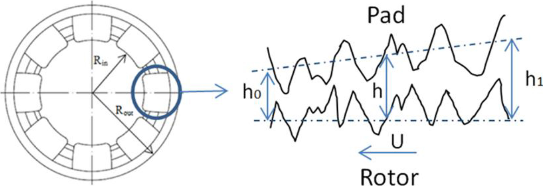

In Eq. (14) $\tau$ ₀ is the Eyring shear stress and is considered to be equal to 2MPa [31], while $\mu$ _asp corresponds to the pressure coefficient of boundary shear strength and is considered to be equal to 0.17 [33].

2.2 Viscosity model

The concept of the “effective temperature” [26] is taken into consideration to approximate the operating viscosity value without applying complex and time consuming THD algorithms. The effective temperature value inside the lubricant’s domain is calculated from Eqs (18) and (19) [26]. The variation of temperature $\Delta$ T during operation depends on the friction force, the shaft’s velocity and the average lubricant flow. The lubricant’s properties must also be included in the calculations. An empirical, exponential equation is then applied according to Eqs (20), (21) to identify the dynamic viscosity of the lubricant for the calculated effective temperature.

$\displaystyle T=T_{0}+k_{e}\Delta T$ (18) $\displaystyle\Delta T=\frac{2f_{\textit{tot}}U}{\textit{nQ}\rho C_{p}}$ (19) $\displaystyle\mu=\mu_{v}e^{A_{s}}$ (20) $\displaystyle A_{s}=C_{2}^{\mu}\left({\frac{1}{{\rm T}}+\frac{1}{C_{1}^{\mu}}}% \right)+C_{3}^{\mu}\left({\frac{1}{{\rm T}}+\frac{1}{C_{1}^{\mu}}}\right)$ (21)

2.3 Numerical analysis

As mentioned before, the hydrodynamic lubrication of a thrust bearing is based on two fundamental principles. First of all, in order to generate a lubrication film capable to carry load, two surfaces must rotate with a relative velocity to each other. In addition, a wedge must be formed between the two surfaces at some relative angle. The one surface is assumed to be rotating at a certain velocity and is usually called the <<runner>> or the <<rotor>>. In pivoted pad thrust bearings, the other surface – also called the <<pad>> – is stationary and is assumed to be rotating only around a fixed point.

There are fundamental assumptions that have been taken into consideration to simplify the analysis. The laminar and isothermal flow of a Newtonian and incompressible lubricant was assumed within the tribo-conjunction without the appearance of cavitation effects. Furthermore, based on the fact that the radius of curvature of the pad’s arcs is such, that if they were to be approximated with small linear line segments, the tendency of a straight line would appear, the pad is simulated with a rectangle that pivots around its center as shown in Fig. 1. The Average Reynolds equation is subsequently solved in the Cartesian coordinates system by applying the numerical procedure of Finite Differences.

Figure 2.

2D Grid of the tilting pad of the thrust bearing with 2,500 finite cells.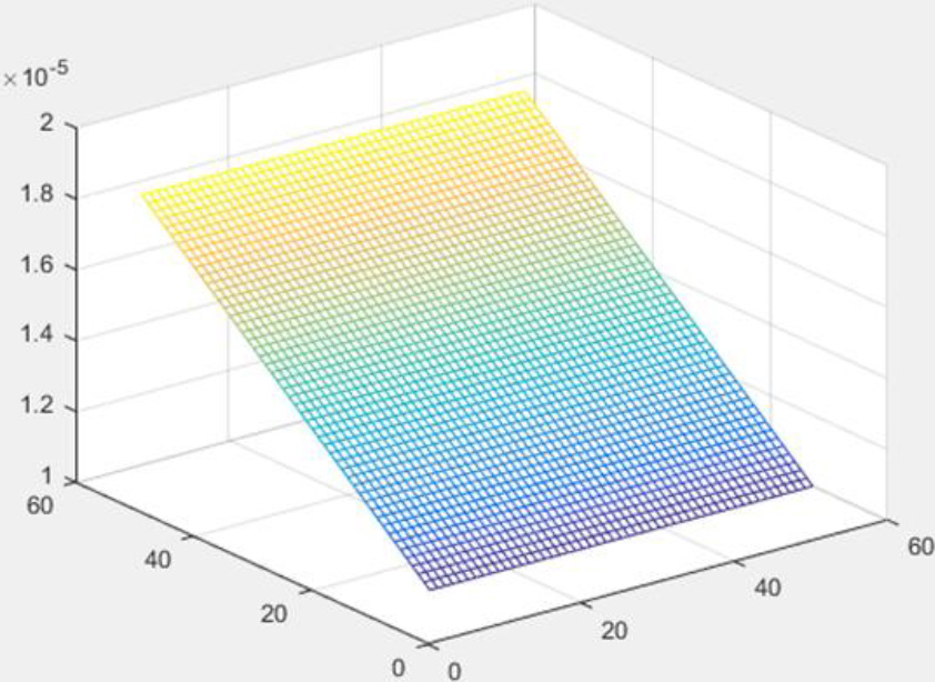

As shown in Fig. 2, a 2D mesh is applied in order to discretize the pad. After a sequence of spatial resolution tests the final mesh consists of 50 finite cells in the direction of the flow and 50 in the cross-flow direction that corresponds to a total number of 2,500 finite cells.

The second step of a numerical analysis includes the definition of the initial and boundary conditions that are essential for the calculations. Initially, an angular velocity, $\omega$ or a linear velocity $U=\omega\times R_{m}$ is applied. $R_{m}$ corresponds to the middle of the pad in the cross-flow direction. This boundary condition is combined with the assumption that there is no slippage in the interface between the rotor and the lubricant. All the free boundaries of the pad are assumed to be openings with a constant pressure $P=p_{\textit{atm}}$ . Moreover, it is assumed that there are no other inflows that affect the fluid film inside the pad-rotor conjunction. During the numerical simulations, the developed hydrodynamic vertical force Eq. (22) that corresponds to the load carrying capacity of the pad is calculated by applying the trapezoidal numerical integration rule on the pressure matrix. Similarly the hydrodynamic friction force Eq. (23) that is developed inside the lubrication film is calculated numerically by integrating the pad’s shear stress over the pad’s surface using the midpoint numerical integration rule.

$\displaystyle W_{h}=\mathop{\sum}\limits_{i=1}^{n_{i}}\mathop{\sum}\limits_{j=% 1}^{m_{j}}P\left({x_{i},y_{j}}\right)\Delta x\Delta y$ (22) $\displaystyle f_{h}=\mathop{\sum}\limits_{i=1}^{n}\mathop{\sum}\limits_{j=1}^{% m}\tau\left({x_{i},y_{j}}\right)\Delta x\Delta y$ (23)

The shear stress is calculated with Eq. (24):

$\displaystyle\tau=\mu\frac{\vartheta u}{\vartheta z}$ (24)

The Average 2-D Reynolds Eq. (1) is modified as shown in Eq. (2.3) for the calculation of the nodal pressure $P_{i,j}$ over the grid [34]. To do so, the derivatives in the differential Reynolds equation are approximated by the truncated Taylor series expansion for three consecutive grid nodes. Based on the central difference form, the values of the function at the neighboring nodes, at both sides of the pole node, are required to calculate the derivatives.

$\displaystyle P_{i,j}=C_{n}P_{n}+C_{s}P_{s}+C_{e}P_{e}+C_{w}P_{w}+G$ $\displaystyle\qquad\quad i,j=0,\ldots,50$ (25)

A Gauss-Seidel iterative algorithm, with a set of linear algebraic equations, is built, based on the above finite difference – central differences methodology. A repetitive procedure of calculations in the flow’s direction is performed until the computed pressure and the inclination of the pad satisfy the convergence criteria.

The Newton-Raphson methodology is applied on the inclination parameter $k$ , Eq. (26), in order to ensure the balance of the tilting pad with the external load.

$\displaystyle k=\frac{h_{1}-h_{0}}{h_{0}}$ (26)

Figure 3.

Iterative computational algorithm flow chart.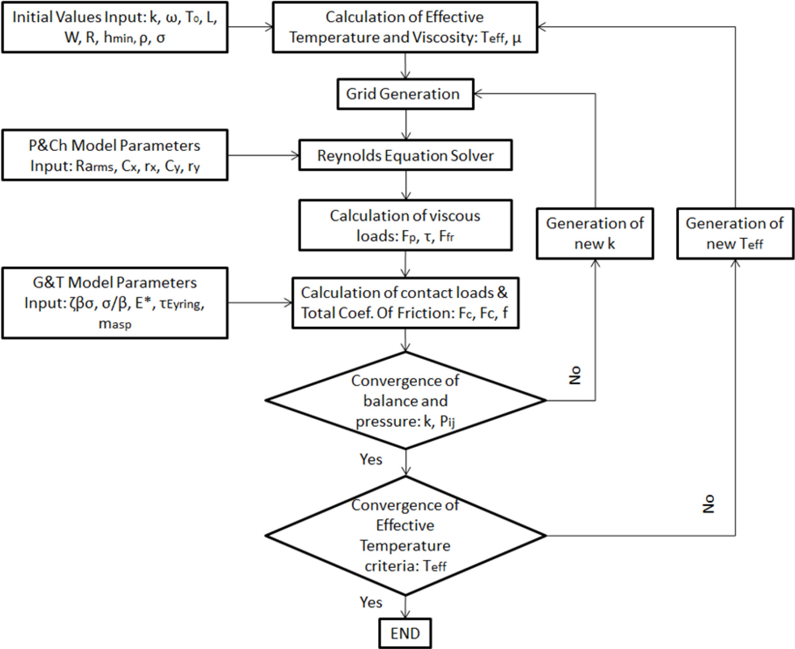

The flow chart shown in Fig. 3 represents the final, complete algorithm that is used to calculate the tribological characteristics of the hydrodynamic tilting pad thrust bearing in mixed lubrication regime. The initial, geometrical and operational characteristics of the simulation are entered and the effective temperature is calculated along with the corresponding dynamic viscosity of the lubricant. Then the grid is generated and the boundary conditions are applied. For the next step the Average Reynolds equation is solved numerically, using the finite difference method, while the flow factors from the model of Patir and Cheng are calculated for transversely oriented rough surface pattern. Applying numerical integrations the viscous load and friction are calculated along with the contact forces from the model of Greenwood and Tripp and then summed to define the total load carrying capacity and friction force for the thrust pad. Finally, two decision nodes are applied. The first, includes the convergence criteria for the calculation of pressure and balance of the pad that returns the algorithm back to the calculation of a new grid. The second includes the convergence criteria of the effective temperatures that lead the algorithm back to a new calculation for the dynamic viscosity. The algorithm ends only when all three convergence criteria are met.

Figure 4.

Numerical versus Experimental specific pad load and minimum film thickness data validation.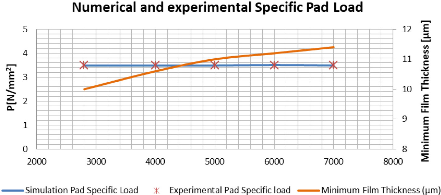

Figure 4 is a graphical representation of the results from the validation process of the numerical algorithm. The data applied for validation derive from the experimental work of Bielec and Leopard [35]. The calculated pressure inside the bearing is compared to the provided experimental results for an increase in rotor’s velocity while the minimum film thickness follows the suggested experimental values. The results show a good agreement between experimental and simulation values.

2.4 Machine learning techniques

Since computer science has been widely developed and applied in many fields over the last decade, a variety of machine learning techniques as well as programming languages and softwares are available to researchers in order to investigate optimum, tailor-made solutions for each specific problem [36, 37]. In the current paper, the thrust bearing’s performance prediction, in mixed lubrication regime, is examined, utilizing Artificial Neural Networks. These smart systems have the ability to learn characteristics of complex systems and give results faster than traditional methods. At the same time, a comparison of the developed ANN is performed to Polynomial Regression models, Support Vector Machines (SVM) Regression Models as well as Regression Trees.

To begin with, Artificial neural networks (ANNs) consist of basic elements that imitate biological nervous systems. In general, the ANNs are submitted to a training procedure of connection-weights aiming to associate specific inputs with specific target values. The ANN training process is done by using pairs of input and output vectors (supervised learning) and is deployed until a convergence is reached. A simple ANN model with a vector of inputs x is presented here. The inputs $x_{1},x_{2},\ldots,x_{R}$ are multiplied by the weight matrix W for M neurons and the weighted values are summed. Each neuron has a bias value b which is summed with the weighted inputs to create the net output $y$ that is used as an argument for the transfer function $f$ .

$\displaystyle n\!=\!W_{1,1}\times p_{1}\!+\!W_{1,2}\times p_{2}\!+\!W_{1,R}% \times p_{R}\!+\!b$ (27)

The transfer function can be selected from a variety of functions, such as linear, tan-sigmoid, log-sigmoid, ReLU etc. A network may have multiple layers and the outputs of each intermediate (hidden) layer are used as inputs for the next layer.

As mentioned earlier, the ANN is undergoing supervised training, in which the learning rule is presented with a set of desired network behavior examples, $\left\{{{x}_{1},{t}_{1}}\right\},\left\{{{x}_{2},{t}_{2}}\right\},\ldots,\left% \{{{x}_{q},{t}_{q}}\right\}$ where ${x}_{q}$ represents the input of the network and $t_{q}$ represents the targeted output. The algorithm aims to minimize the mean error sum by adjusting neural network weights and biases.

The second machine learning methodology examined in the current paper is the Quadratic Polynomial Regression. Equation (28), describes the relationship between one response variable $y$ and two predictors $x_{1},x_{2}$ as a simple, linear line or plane surface (depending on the number of the predictors) with slope $\beta$ ₁, $\beta$ ₂ and y-intercept $\beta$ ₀:

$\displaystyle y=\beta_{0}+\beta_{1}x_{1}+\beta_{2}x_{2}+\varepsilon$ (28)

Equations (29) and (30) describe in matrix form the system that needs to be solved for a dataset of n-observations to derive the corresponding regression model and calculate $\beta_{0}$ , $\beta_{1}$ , $\beta_{2}$ :

$\displaystyle Y=\left[{{\begin{array}[]{c}{y_{1}}\\ {y_{2}}\\ \vdots\\ {y_{N}}\\ \end{array}}}\right]=\left[{\begin{array}[]{ccc}1&{x_{11}}&{x_{21}}\\ 1&{x_{12}}&{x_{22}}\\ \vdots&\vdots&\vdots\\ 1&{x_{1N}}&{x_{2N}}\\ \end{array}}\right]\left[{{\begin{array}[]{c}{\beta_{0}}\\ {\beta_{1}}\\ {\beta_{2}}\\ \end{array}}}\right]$ (29)

$\displaystyle Y=\textit{XB}$ (30)

For the application of a quadratic polynomial regression model, the $X$ matrix of Eq. (31) is generated.

$\displaystyle X=\left[\begin{array}[]{cccccc}1&{x_{11}}&{x_{21}}&{x_{11}^{2}}&% {x_{11}x_{21}}&{x_{21}^{2}}\\ 1&{x_{12}}&{x_{22}}&{x_{12}^{2}}&{x_{12}x_{22}}&{x_{22}^{2}}\\ \vdots&\vdots&\vdots&\vdots&\vdots&\vdots\\ 1&{x_{1N}}&{x_{2N}}&{x_{1N}^{2}}&{x_{1N}x_{2N}}&{x_{2N}^{2}}\\ \end{array}\right]$ (31)

Equation (2.4) represents the final model in matrix form.

$\displaystyle Y=\left[\begin{array}[]{c}y_{1}\\ y_{2}\\ \vdots\\ y_{N}\end{array}\right]$ $\displaystyle=\left[\begin{array}[]{ccccccc}1&x_{11}&x_{21}&x_{11}{}^{2}&x_{11% }x_{21}&x_{21}{}^{2}\\ 1&x_{12}&x_{22}&x_{12}{}^{2}&x_{12}x_{22}&x_{22}{}^{2}\\ \vdots&\vdots&\vdots&\vdots&\vdots&\vdots\\ 1&x_{1N}&x_{2N}&x_{1N}{}^{2}&x_{1N}x_{2N}&x_{2N}{}^{2}\end{array}\right]\!\!% \left[\begin{array}[]{c}\beta_{0}\\ \beta_{1}\\ \beta_{2}\\ \beta_{3}\\ \beta_{4}\\ \beta_{5}\end{array}\right].$ (32)

The least square method (LSM) [38] is used to identify the best fit curve or line for one set of data points by reducing the sum of the squared residuals of the points of the curve. As a result the corresponding slopes ( $\beta)$ and y-intercepts of the final model are calculated based on this regression surface.

The third machine learning method examined is the Quadratic Support Vector Machine Regression. Support vector machines (SVM) is a supervised learning algorithm mainly applied for classification and regression problems as support vector classification (SVC) and support vector regression (SVR). SVM was first identified by Vladimir Vapnik et al. on 1992 [39] and it is usually applied for smaller datasets as it takes too long to process. There are cases where the data do not allow a linear model to be built. In these cases a non-linear SVM regression model is built based on the nonlinear kernel functions. For the current investigation, the polynomial kernel function Eq. (33) is applied for the $2^{\text{nd}}$ (Quadratic) degree ( $q=2)$ .

$\displaystyle G\left({X,Y}\right)=\left({c+X^{T}Y}\right)^{q}$ (33)

The final machine learning method investigated is the Fine Trees. CART- Regression Trees belong to the general family of Decision Trees and were originally developed by Breiman et al. on 1984 [40].

Figure 5.

Regression model validation with experimental data.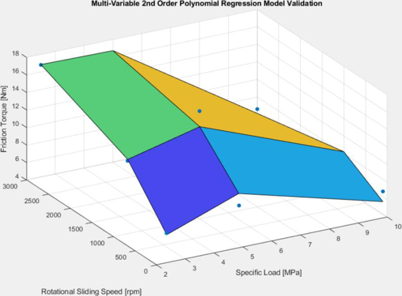

A classification or regression decision tree is used as a predictive model to draw conclusions about a set of n-observations. To perform the analysis of the current investigation all the data must be sorted in ascending order for both predictors $x_{1i},x_{2i}$ . Then all the mean squared errors are calculated separately for all the response values of both predictors Eq. (34) in each splitting candidate node $t$ . A repetitive procedure calculates the internal nodes of the Fine Tree until each branch has no less than 4 observations to split.

$\displaystyle\textit{MSE}=\mathop{\sum}\nolimits\frac{1}{N}\left({y_{i}-% \overline{y_{\textit{fit}_{t}}}}\right)^{2}$ (34)

When training a model, it is important not to over-fit or under-fit it. The choice of training set and test set is critical in reducing this risk. However, dividing the dataset to maximize both learning and validity of test results is difficult. For the current investigation the k-fold cross validation technique is applied as one of the most popular methodologies to randomly partition data. With a value of $k=$ 5, the method partitions the dataset in 5 random subsets. 80% of the data are used for training and testing while the rest 20% is used for for validation.

The goodness of fit for the generated models is determined by calculating the corresponding $R^{2}$ with Eq. (35). $R^{2}$ can take values between the numbers 0 to 1 and the model with the highest calculated value is the one that best fits the dataset.

$\displaystyle R^{2}=1-\frac{\mathop{\sum}\nolimits_{1}^{N}\left({y_{i}-y_{% \textit{fit}}}\right)^{2}}{\mathop{\sum}\nolimits_{1}^{N}\left({y_{i}-\bar{y}}% \right)^{2}}$ (35)

A validation procedure of the developed Quadratic Polynomial Regression algorithm was followed based on experimental data from Michal Wasilczuk et al. [41]. Figure 5is graphical representation of the generated model in comparison to the dataset. The calculated coefficient of determination for the case study is 0.944 and the regression model is presented in Eq. (2.4):

$\displaystyle{y}=-0.53+0.009{x}+3.3{z}-0.14\cdot 10^{-5}{x}^{2}$ $\displaystyle\qquad-0.0004{xz}-0.28{z}^{2}$ (36)

In summary, a numerical analysis algorithm is developed in order to solve the mixed lubrication problem of a tilting pad thrust bearing. The algorithm is solved for various operating conditions and coatings. The simulation data are gathered and used in order to train ML models able to predict the friction coefficient of the bearing with high accuracy and remarkable speed.

3. Results and discussion

Table 1
Lubricants’ properties

	SAE 0W30	SAE 10W40	SAE 10W60
Dynamic viscosity @50oC [Pasec]	0.038	0.054	0.088
Density @40oC [Kg/m3]	835	917	841
Specific heat capacity [J/kgK]	2050	1980	1901

Table 2

Coating’s properties

	Steel	CrN	TiN	TiAlN	DLC
Young’s modulus of elasticity [Gpa]	200	400	250	291	300
Poisson’s ratio	0.31	0.2	0.25	0.22	0.25
Surface roughness [ $\mu$ m]	0.4	0.25	0.31	0.059	0.033
Roughness parameter ( $\zeta\kappa\sigma)$	0.074	0.065	0.064	0.053	0.052
Asperity slope ( $\sigma$ / $\kappa)$	0.0105	0.0101	0.0172	0.0161	0.0132

Table 3

General input data

Input parameter	Value	Unit
Pad’s length	32	mm
Pad’s width	28	mm
Pad’s outer radius	62	mm
Lubricant’s inlet temperature	323	K
Steel shaft’s surface roughness	1.7	$\mu$ m
$C_{\Phi x}$	1.18
$C_{\Phi y}$	0.225
$r_{\Phi x}$	0.42
$r_{\Phi y}$	1.5

Table 4

$R^{2}$ results for the trained ANN models

	${R}^{2}$
ANN SAE 0W30	0.96
ANN SAE 10W40	0.98
ANN SAE 10W60	0.97

The numerical analysis simulations were performed for sliding shaft speeds of 0.5 m/s to 5 m/s and external applied load on the pad 8450N. Three lubricants were used for the simulations: SAE 0W30, SAE 10W40 and SAE 10W60. In addition, all simulations were performed for a steel shaft, a plain steel pad as well as 4 different coated pads with TiN, CrN, TiAlN and DLC. The flow factors’ parameters were defined from Patir & Cheng’s model for a transversely oriented surface with $\gamma=$ 1/3 and $\lambda=$ 1.94–1.63 $>$ 1. All the input parameters of the investigation are summarized in Tables 1, 2 and 3.

Figure 6.

Problem formulation flow chart.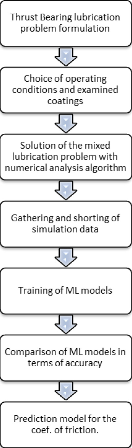

Figure 7.

Typical pad pressure distribution.

A typical pressure distribution from the numerical analysis of the pad bearing is shown in Fig. 7.

Figure 8.

Variation of the pressure flow factors $\Phi_{x}$ , $\Phi_{y}$ according to $\lambda$ .

Moreover, the variation of the pressure flow factors $\Phi$ _χ and $\Phi$ _y according to $\lambda$ is presented in Fig. 8.

It is clear that while $\lambda$ decreases, so does the pressure flow factor $\Phi$ _x. The results agree with the ones shown in the paper of Patir and Cheng as well as with the fact that the asperities start interacting with each other, as $\lambda$ decreases from 1.94 to 1.63, creating obstructions to the normal flow and resulting in drop of the pressure flow, hence to the pressure flow factors.

Figure 9.

Loss function of ANN during training epochs (SAE W40).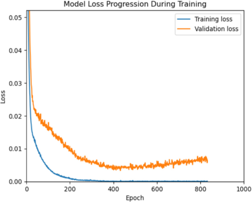

There are many different ANN types with different topologies. The one that will be used in this study is a feed-forward multilayer perceptron. The choice of the feed-forward multilayer perceptron is due to its simple nature and the accuracy of the results. The regression neural network consists of two inputs and one output. The inputs are the coatings (Young’s Modulus in GPa) and the velocity (m/s) of the rotor. The loss function is the ‘mean squared error’, the optimization algorithm is the ‘Adam’, the activation function for hidden layers is ReLU and the output layer is the ‘linear’. The network has one hidden layers with 20 neurons. The dataset for the NN was created for different velocities and Young Modulu’s values while the total number of samples is 60 for each lubricant. Of these data, 60% have been used for training, 20% for validation and the last 20% for testing. The output of the network is the coefficient of friction. A typical representation of the model loss progression during training is shown in Fig. 9.

Figure 10.

Comparison of ANN and simulation values for SAE 0W30.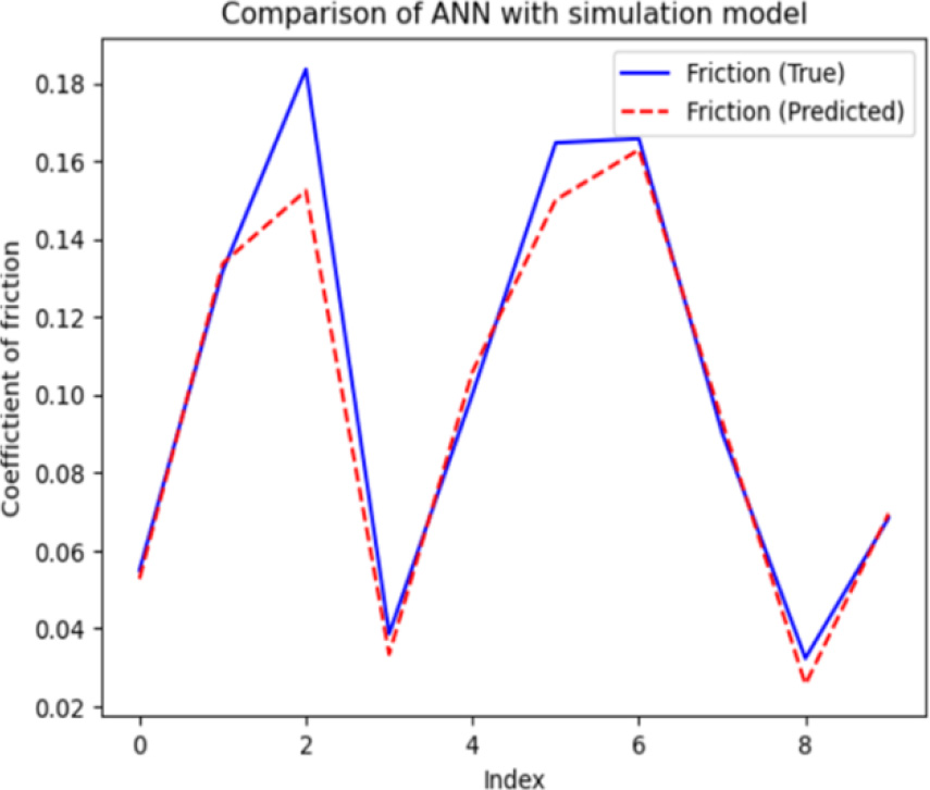

Figure 11.

Comparison of ANN and simulation values for SAE 10W40.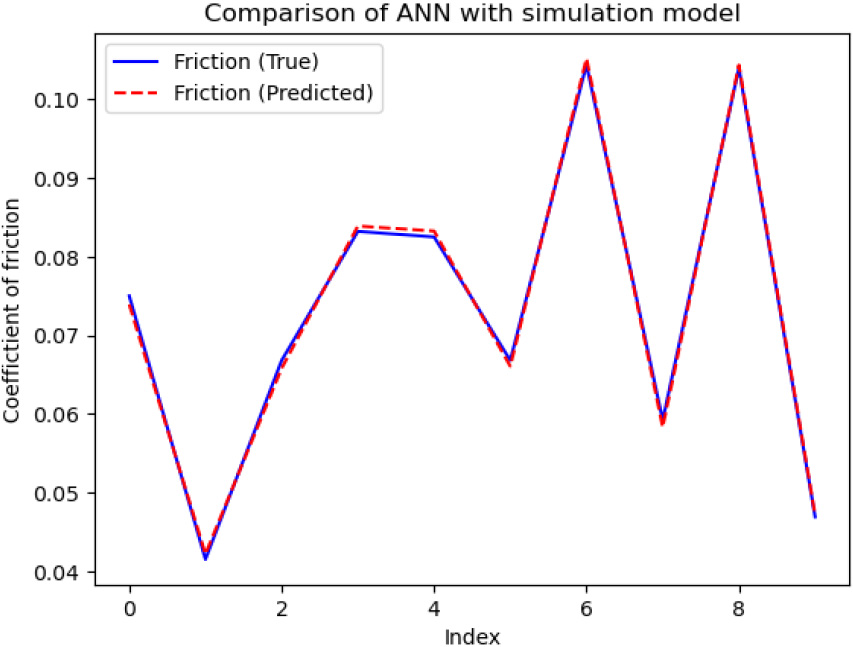

Figure 12.

Comparison of ANN and simulation values for SAE10W60.

Table 5

Quadratic regression ML models

Case study	ML model	R²
SAE 0W30	$y=0.467-0.322\times 10^{-1}-0.210\times 10^{-2}x_{2}+0.157\times 10^{-2}x_{1}^% {2}+0.138\times 10^{-4}x_{1}x_{2}-0.326\times 10^{-5}x_{2}^{2}$	0.87
SAE 10W40	$y=0.466-0.321\times 10^{-1}-0.210\times 10^{-2}x_{2}+0.161\times 10^{-2}x_{1}^% {2}+0.138\times 10^{-4}x_{1}x_{2}-0.326\times 10^{-5}x_{2}^{2}$	0.87
SAE 10W60	$y=0.465-0.319\times 10^{-1}x_{1}-0.209\times 10^{-2}x_{2}+0.165\times 10^{-2}x% _{1}^{2}+0.141\times 10^{-4}x_{1}x_{2}-0.324\times 10^{-5}x_{2}^{2}$	0.87

Figure 13.

Multivariable quadratic polynomial regression models response plot.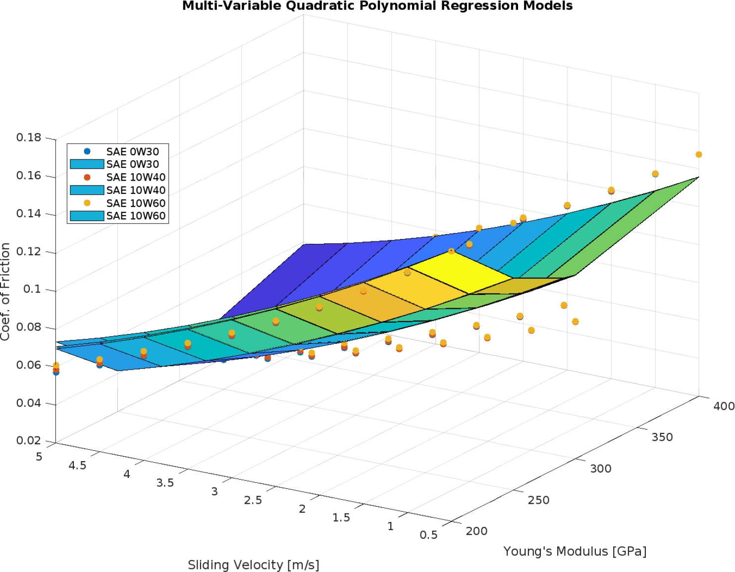

The trained ANN models showed a very good fitting in the simulation data. The ANN metrics of all the ANN models are gathered in Table 4. The comparison of ANN results and simulation values for the three lubricants are represented graphically in Figs 10, 11 and 12.

Figure 14.

Quadratic SVM model SAE 10W40 response plot for sliding velocity.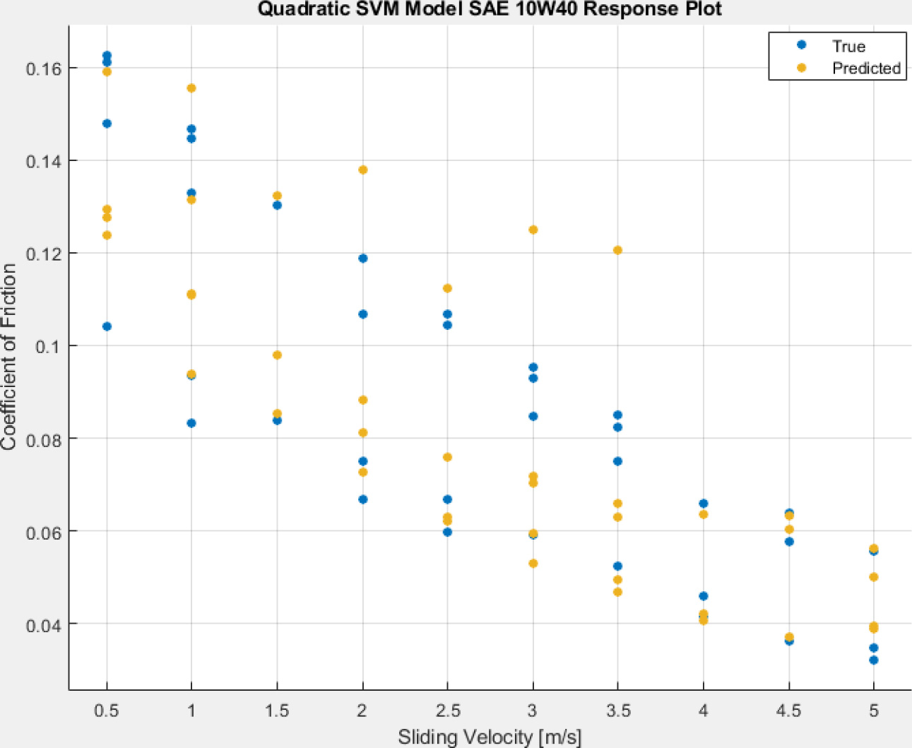

Figure 15.

Quadratic SVM model SAE 10W40 response plot for Young’s Modulus.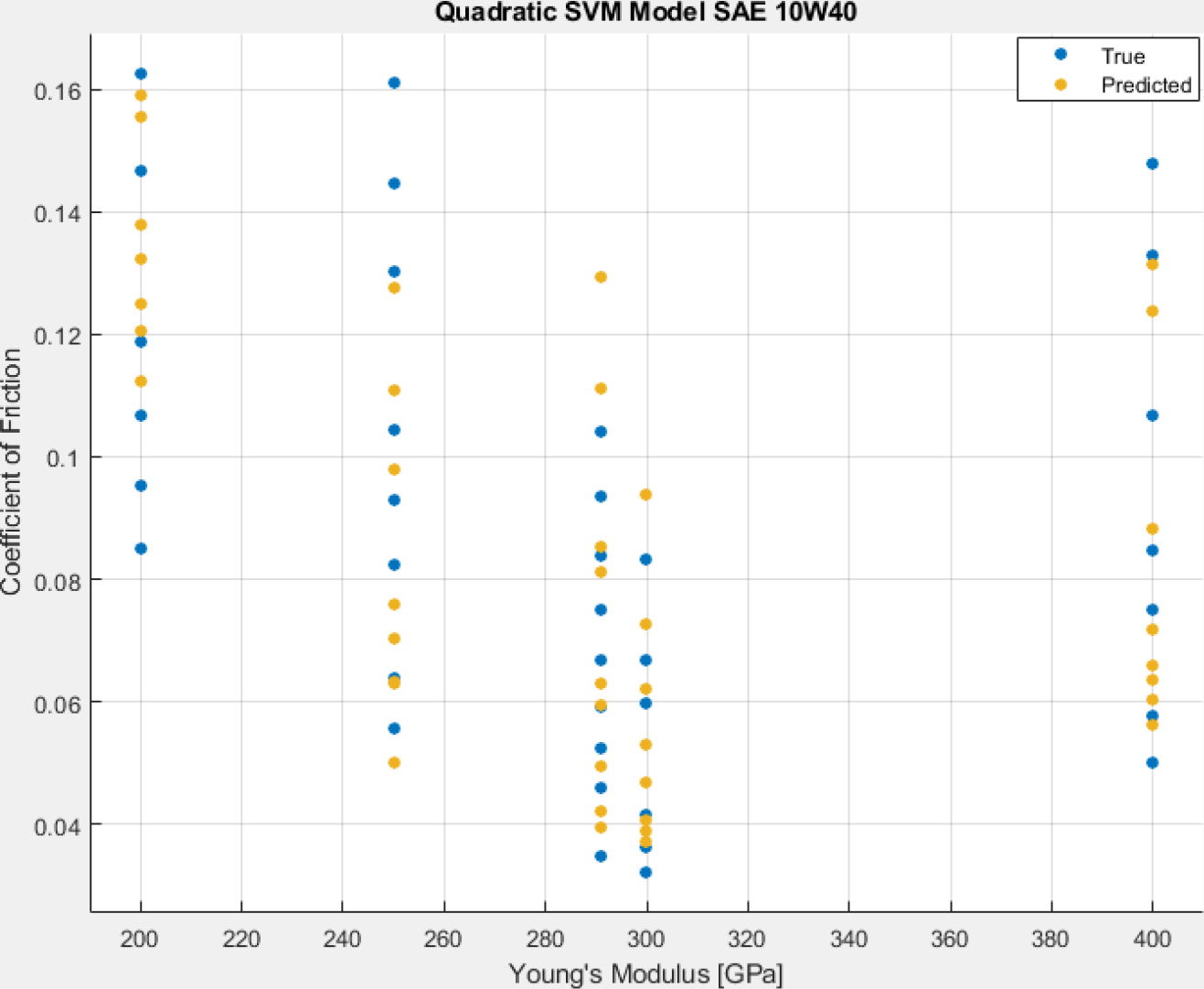

Figure 16.

Typical Fine Tree ML model for SAE 10W40.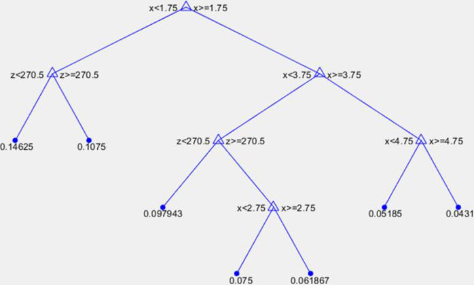

Overfitting is a common problem in machine learning. Overfitting means that the model is over trained on the training data set, resulting in weights adjusted to the noise in the training data instead of learning “a general predicting rule” [42].

In order to achieve better performance of the networks and avoid overfitting several methods were applied during the training such as early stopping, feature scaling and decaying learning rate of the optimization algorithm [43]. Specifically, the early stopping method stops the training, after a number of optimization steps that do not lead to a decreased validation loss. Feature scaling can be done for the whole dataset during the preprocessing stage and it means that every feature in the dataset is scaled independently in the range 0–1.

A variety of different ANN architectures was tested following a trial-and-error process to determine the most efficient one for the current system. The examined networks were evaluated for different numbers of layers, neurons and activation functions in order to identify the architecture that provided optimum performance while avoiding overfitting. A different combination of hyperparameters for the ANNs is possible to provide even higher coefficient of determination and even lower error. Nevertheless, with R² varying from 0.96–0.98, the results achieved with the developed ANNs in this study can be characterized as efficient. The results show that, based on the velocity and Young Modulus’s value, the coefficient of friction can be fully estimated with great accuracy. The calculation of the coefficient of friction using the ANN methodology is the key point of this work.

The next ML models that were created from the numerical analysis data were based on Quadratic Polynomial Regression. The results for the three lubricants SAE 0W30, SAE 10W40 and SAE 10W60 are shown in Table 5. All models use two independent predictors: $x_{1i}$ for the sliding velocity and $x_{2i}$ for the coating’s Young’s Modulus, in order to predict the response variable $y_{i}$ that represent the coefficient of friction.

Table 6

SVM and Fine Tree ML models R² values

Model	R²
Quadratic SVM SAE 0W30	0.83
Quadratic SVM SAE 10W40	0.82
Quadratic SVM SAE 10W60	0.85
Fine tree SAE 0W30	0.74
Fine tree SAE 10W40	0.61
Fine tree SAE 10W60	0.56

Figure 13is the representation of the generated regression surfaces. The dots represent the simulation values while the surfaces represent the regression models developed with the LSM for all three lubricants, sliding velocities and coatings – represented with their corresponding Young’s Modulus values. It is easily noted that the drop of the sliding velocity leads in rise of the coefficient of friction in both cases. It is true that as the velocity drops so does the minimum film thickness and the amount of lubricant flowing inside the mechanism. As a result, the hydrodynamic characteristics of the bearing and the viscous friction do not have a significant impact on the final performance. However, the contact of the two surfaces that come closer as the minimum film thickness wanes, gain a leading role on the total amount of friction that is developed within the conjunction. At this point, the material of the surfaces that come in contact has a significant impact on the coefficient of friction. From Fig. 13, it can be seen that rough materials like steel and CrN show large coefficient of friction values, while the smoother materials do help the mechanism operate with lower friction. In all studies cases the DLC coating shows up to 45% better performance in terms of low coefficient of friction values. At the same time the three lubricants, although with a notable difference in viscosity, show similar behavior, due to the fact that the viscous forces do not affect the performance of the bearing significantly, as $\lambda$ drops from 1.94 to 1.63.

For comparison purposes the same data sets were used in Matlab’s Regression Learner application in order to train Quadratic SVM and Fine Tree Regression models. The results of these models are summarized in Table 6.

Typical response plots for the quadratic SVM model of SAE10W40 are shown in Figs 14 and 15.

Finally, a typical Fine Tree model for SAE 10W40 is shown in Fig. 16.

Table 7

Comparison table of ML models based on R²

Model	R²
Artificial neural network	97
Polynomial regression	87
Support vector machines	83
Fine tree	64

Figure 17.

Comparison of the ML methods in terms of fit to the dataset using the coefficient of determination [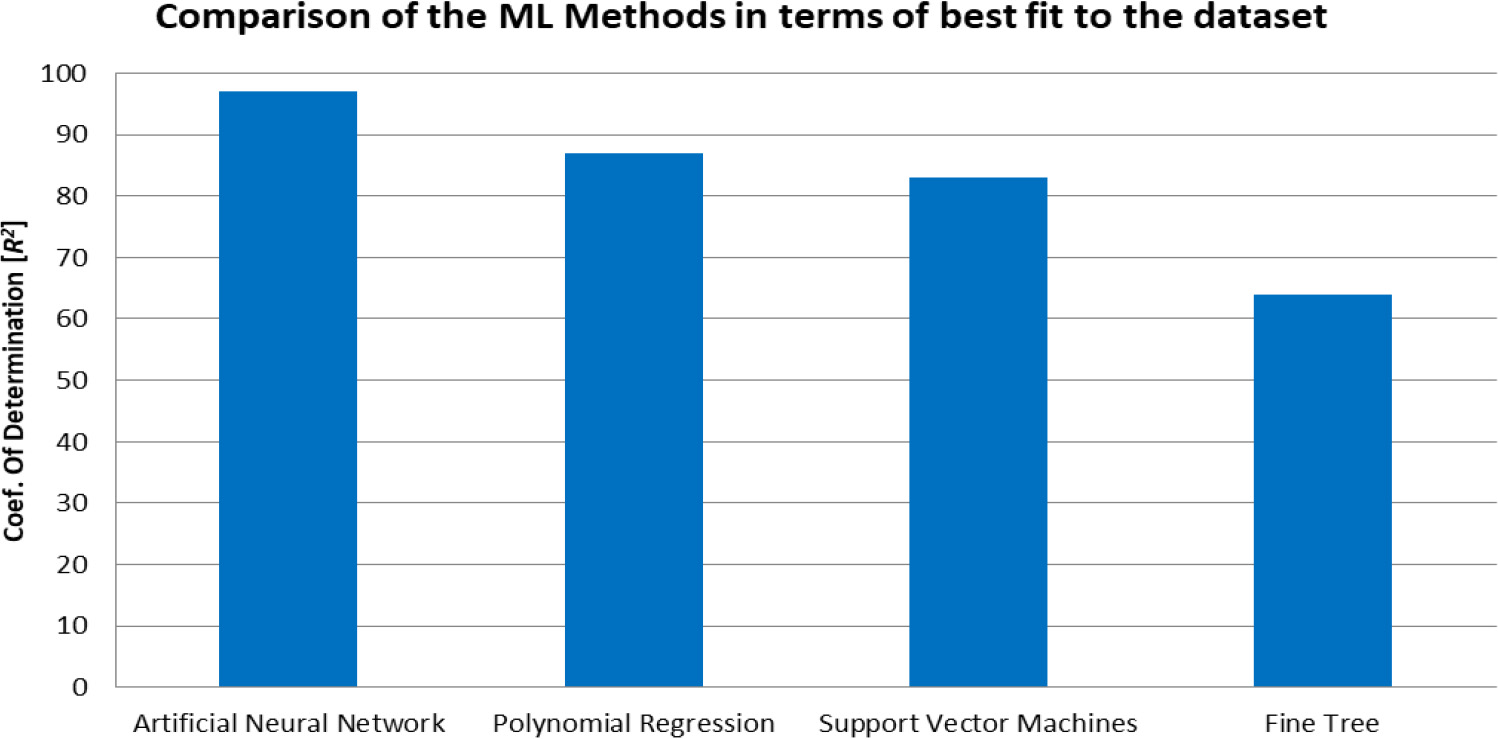 $R^{2}$ ].

The coefficient of determination $R^{2}$ is the value that shows how good the fit of the models to the numerical data is. The Fine Tree models for all lubricants show the lowest $R^{2}$ values and do not have a good fit to the data sets. The SVM models are slightly worse than the Quadratic Polynomial Regression models with all R² values varying around 0.85. Finally, based on R², the ANN models show the best fit of all with the respective values varying around 0.97. Table 7 and Fig. 17summarize the outcome of the investigation. In conclusion the ANN models developed in the current investigation are the best from the ones examined in terms of predicting the coefficient of friction for a thrust pad operating in mixed lubrication regime based on the sliding velocity and the applied coating.

4. Conclusions

For the current investigation, a pivoted pad thrust bearing was simulated in mixed lubrication regime for various speeds, lubricants and applied coatings. All the simulation data were then used in order to train machine learning models able to predict the coefficient of friction based on velocity and coating as inputs. In that way the modeling of thrust bearings’ lubrication can evolve from analytical and time consuming numerical models to ML models that are fast and provide accurate results when trained properly.

Summarizing the results from the tribological perspective, all the lubricants were found to have an almost similar coefficient of friction in mixed lubrication regime because as the velocity of the rotor reduced, the viscous loads tended to have lower impact on the final performance of the bearing while the contact forces played the major role. In addition, the DLC coating, having the least roughness of all, showed the best tribological performance for the tilting thrust bearing pad reaching up to 45% reduction for the friction coefficient compared to the rest of the coated and uncoated surfaces.

From the Machine Learning perspective, the R² was the metric chosen in order to compare the various machine learning models in terms of best fit in the simulation data that would eventually provide the best prediction model. The machine learning models that were examined during the investigation include Artificial Neural Networks, Quadratic Polynomial Regression models, Support Vector Machines and Decision Trees. From all the examined models the ANN were the ones that showed the highest R² values and are suggested as the most suitable in order to build performance prediction models for pad thrust bearings in mixed lubrication regime.

As future extension of the current research, meta-algorithmic methods [44] could be investigated and compared along with various architectures of ANNs. To add to that, recent trends indicate that the development of Physics-informed neural networks (PINNs) [45, 46] could be a potential solution to the presented problem and should be taken into consideration for future applications in mixed lubrication bearings’ problems. Finally, more sophisticated supervised machine learning algorithm such as Neural Dynamic Classification algorithms, Dynamic Ensemble Learning Algorithms, Finite Element Machines for fast learning and self-supervised learning [47, 48, 49, 50] appear to be of great interest regarding future research related to the presented problem but also generally for applications in the field of Tribology.

Footnotes

Acknowledgments

The publication fees of this manuscript have been financed by the Research Council of the University of Patras.

Nomenclature

$A$ :	Pad’s surface [m²]
$A_{c}$ :	Apparent contact area [m²]
$B$ :	pad length in x-direction [m]
$C$ :	Empirical Coefficient according to surface orientation for rough surfaces
$C_{1}^{\mu}$ :	first viscosity coefficient – absolute temperature at which $\mu=\mu_{\nu}$ (323 K)
$C_{2}^{\mu}$ :	second viscosity coefficient according to Sutherland’s law $=$ 3,800
$C_{3}^{\mu}$ :	third viscosity coefficient according to Sutherland’s law $=$ 30,000
$C_{n,s,w,e}$ :	constants for each neighbor node: north, south, west, east
$c_{p}$ :	Specific Heat [J/kgK]
$E$ :	Expectancy operator
$f_{\textit{tot}}$ :	Total friction force [N]
$f_{h,c}$ :	Hydrodynamic and Contact friction force [N]
$h$ :	film thickness [m]
$h_{0},h_{1}$ :	outlet, inlet film thickness [m]
$h_{i}$ :	Nodal film thickness [m]
$h_{\min}$ :	minimum film thickness [m]: $h_{\min}={\min}$ $\left({h_{0},h_{1}}\right)$
$i$ :	Descrite variable for node definition in the direction of the flow
$i_{b}$ :	Iterations counting variable for Newton Raphson algorithm on $k$
$j$ :	Descrite variable for node definition in the cross – flow direction
$k$ :	convergence ratio: $k=\left({h_{1}-h_{0}}\right)/h_{0}$
$k_{e}$ :	Empirical constant for good agreement between theory and experiment $=$ 0.8 [21]
$L$ :	pad’s width in y-direction [m]
$l_{1,2}$ :	Variable lubricant’s width [m]
$l_{\textit{in}}$ :	Inlet lubricant width [m]
$l_{\textit{in}_{1,2}}$ :	Start (1) and end (2) lubricant’s positions in the pad’s inlet area [m]
$m_{j}$ :	Total number of nodes in j direction
$n$ :	Fraction of oil film coverage on the leading edge of the pad
$n_{i}$ :	Total number of nodes in i direction
$P$ :	absolute nodal pressure [Pa]
$p$ :	absolute pressure [Pa]
$p_{\textit{atm}}$ :	Atmospheric pressure [Pa]
$Q$ :	Lubricant flow [m³/h]

$Q_{\textit{in,out}}$ :	Lubricant flow in inlet and outlet area of the pad [m³/h]
$Q_{\textit{sr1,2}}$ :	Lubricant outflow from the sides of the pad [m³/h]
$q_{x,y}$ :	Lubricant flow in x and y directions [m³/h]
$R_{\textit{in, out}}$ :	Inner and Outer pad’s radious [m]
$R_{\textit{in}_{1,2}}$ :	Inlet Pad Radious for the beginning of the lubrication film’s width [m]
$R_{m}$ :	Pad radious at mid sector [m]
$r$ :	Empirical Coefficient according to surface orientation for rough surfaces
$T$ :	temperature [K]
$T_{0}$ :	Inlet temperature [K]
$T_{\textit{eff}}$ :	Effective Temperature [K]
$t$ :	Time [sec]
$U$ :	linear rotor velocity [m/s]
$u$ :	Velocity along x axis [m/s]
$V$ :	Volume [m³]
$W_{\textit{tot}}$ :	Total load carrying capacity [N]
$W_{h,c}$ :	Hydrodynamic and Contact load [N]
$x$ :	Independent length variable in the direction of the flow [m]
$y$ :	Independent length variable in the cross (radial) direction of the flow [m]
$z$ :	Independent length variable on the vertical axis of the flow [m]
$\beta$ :	Average asperity radious [m]
$\gamma$ :	Ratio of longitudional and transverse correlation lengths of the asperities
${\rm E}^{*}$ :	Composite Young Modulus [Pa]
$E$ :	Young Modulus of Elasticity [Pa]
$\zeta$ :	Surface density of the asperity peaks
$\lambda$ :	Fraction of minimum film thickness and composite surface roughness commonly used to define the lubrication regime.
$\mu$ :	dynamic viscosity coefficient [Pasec]
$\mu_{v}$ :	nominal dynamic viscosity [Pasec]
$\mu_{\textit{asp}}$ :	Coefficient of boundary shear strength
$\mu_{f}$ :	Coefficient of friction
$v$ :	Poisson’s ratio
$\rho$ :	Density [kg/m³]
$\sigma$ :	Composite (RMS) surface roughness [ $\mu$ m]
$\sigma_{p,r}$ :	Surface roughness for the pad (p) and the rotor (r)
$\tau$ :	Shear stress [Pa]
$\tau_{0}$ :	Eyring shear stress [Pa]
$\Phi_{x,y}$ :	Pressure Flow Factors
$\omega$ :	Rotational Velocity [rpm]

References

Kalsi

Alvarez

Somogyi

Richie

. Load-responsive hydrodynamic bearing for downhole drilling tools. Journal of Tribology. 2007; 129(1): 209-217.

Lingwall

Cooley

Sexton

. Polycrystalline diamond thrust bearing testing and qualification for application in marine hydrokinetic machines. American Society of Mechanical Engineers, Tribology Division, TRIB. 2012; 221-223.

Sun

Zhang

Wei

Wang

. Stability analysis of rubber-supported thrust bearing in a rotor-bearing system used in marine thrusters under disturbing moments. Tribology International. 2020; 151: art. no. 106356.

Etsion

. Improving tribological performance of mechanical components by laser surface texturing. Tribology Letters. 2004; 17(4): 733-737.

Knuteson

Sexton

Cooley

. Wear-in behaviour of polycrystalline diamond thrust bearings. Wear. 2011; 271(9–10): 2106-2110.

Khonsari

. Investigation of tribological behaviors of annular rings with spiral groove. Tribology International. 2011; 44(12): 1610-1619.

Zhang

Gao

Yin

Wang

Gao

. Numerical analysis and experimental research on load carrying capacity of water-lubricated tilting-pad thrust bearings. Mechanics and Industry. 2018; 19(2): art. no. 201.

Wang

Kato

Adachi

Aizawa

. Loads carrying capacity map for the surface texture design of SiC thrust bearing sliding in water. Tribology International. 2003; 36(3): 189-197.

Illner

Bobach

Bartel

Deters

. Simulation of a thrust bearing in a diesel injection pump under mixed lubrication conditions. World Tribology Congress. 2009; Proceedings: 44.

10.

Henry

Bouyer

Fillon

. Experimental analysis of the hydrodynamic effect during start-up of fixed geometry thrust bearings. Tribology International. 2018; 120: 299-308.

11.

Rodriguez-Galiano

Sanchez-Castillo

Chica-Olmo

Chica-Rivas

MJOGR

. Machine learning predictive models for mineral prospectivity: An evaluation of neural networks, random forest, regression trees and support vector machines. Ore Geology Reviews. 2015; 71: 804-818.

12.

Fernandes

Morais

Vale

. Near real-time management of appliances, distributed generation and electric vehicles for demand response participation. Integr. Comput. Aided Eng. 2022; 29(4): 351-366.

13.

Wang

Kiritsis

. Cognitive twin construction for system of systems operation based on semantic integration and high-level architecture. Integr Comput Aided Eng. 2022; 29(3): 277-295.

14.

Yun

Park

. Modal identification of building structures under unknown input conditions using extended Kalman filter and long-short term memory. Integr Comput Aided Eng. 2023; 30(2): 185-201.

15.

Ruiz

Diaz

Gonzales

Cavas-Martinez

. Improving the competitiveness of aircraft manufacturing automated processes by a deep neural network. Integr Comput Aided Eng. 2023; 30(4): 341-352.

16.

Uridales

Matin

Armingol

. An improved deep learning architecture for multi-object tracking systems. Integr Comput Aided Eng. 2023; 30(2): 121-134.

17.

Marian

Tremmel

. Current Trends and Applications of Machine Learning in Tribology – A Review. Lubricants. 2021; 9: 86.

18.

Alves

Daniel

Fiori de Castro

Machado

Cavalca

Gecgel

Dias

Ekwaroosire

. Uncertainty quantification in deep convolutional neural network diagnostics of journal bearings with ovalization fault. Mechanism and Machine Theory. 2020; 149: 103835.

19.

Lorza

García

Martínez

. Combination of the finite element method and data mining techniques to design and optimize bearings. International Joint Conference SOCO’14-CISIS’14-ICEUTE’14. Advances in Intelligent Systems and Computing. 2014; 299: 165.

20.

Lorza

Garcia

Martinez

. Using the finite element method and data mining techniques as an alternative method to determine the maximum load capacity in tapered roller bearings. Journal of Applied Logic. 2017; 24(Part A): 4-14.

21.

Rossopoulos

Papadopoulos

. A journal bearing performance prediction method utilizing a machine learning technique. Proceedings of the Institution of Mechanical Engineers, Part J: Journal of Engineering Tribology. 2021; 13506501211055710.

22.

Kokkinidis

Nikolakopoulos

. Simulation of misaligned journal bearing using neural network. Tribology in Industry. Article in press. 2022; 44(1): 183-197.

23.

Katsaros

Nikolakopoulos

. A combined Machine Learning and Computational methodology for optimum Thrust Bearings’ behavior in mixed lubrication regime. 1st Olympiad in Engineering Science Conference. Greece. 2023 May.

24.

Stachowiak

Batchelor

. Engineering Tribology. 1993.

25.

Tala-Ighil

Fillon

. A numerical investigation of both thermal and texturing surface effects on the journal bearings static characteristics. Tribology International. 2015; 90: 228-239.

26.

Patir

Cheng

. An average flow model for determining effects of three-dimensional roughness on partial hydrodynamic lubrication. Transactions of the ASME. 1978; 12: 100.

27.

Greenwood

Tripp

. The contact of two nominally flat rough surfaces. Proceedings of the Institution of Mechanical Engineers. 1970; 185(1): 625-633.

28.

Johnson

Greenwood

Poon

. A simple theory of asperity contact in elastohydrodynamic lubrication. Wear. 1972; 19: 91-108.

29.

Gohar

. Elastohydrodynamics. Ellis Horwood Limited. 1988.

30.

Greenwood

Williamson

JBP

. Contact of Nominally Flat Surfaces. Proceedings of the Royal Society of London. Series A. 1966; 295: 300-319.

31.

Teodorescu

Balakrishnan

Rahnejat

. Integrated tribological analysis within a multi-physics approach to system dynamics. Tribology and Interface Engineering Series (Elsevier). 2005; 48: 725-737.

32.

Arcoumanis

Ostovar

Mortimer

. Mixed lubrication modeling of Newtonian and shear thinning liquids in a piston-ring configuration. SAE Technical Paper Series. No. 972924; 1997.

33.

Teodorescu

Taraza

Henein

. Simplified elasto-hydrodynamic friction model of the cam-tappet contact. SAE World Congress, Detroit, Michigan. 2003 March 3–6.

34.

Ettles

. The development of a generalized computer analysis for sector shaped tilting pad thrust bearings. ASLE Transactions. 1976; 19(2): 153-163.

35.

Bielec

Leopard

. Tilting pad thrust bearings: Factors affecting performance and improvements with directed lubrication. Proceedings of the Institution of Mechanical Engineers. Conference Proceedings. 1969; 184(12): 93-102.

36.

Somvanshi

Tambade

Chavan

Shinde

. A Review of Machine Learning Techniques using Decision Tree and Support Vector Machine. International Conference on Computing Communication Control and automation (ICCUBEA), Pune, India. 2016; 1-7.

37.

Maulud

Abdulazeez

. A Review on Linear Regression Comprehensive Machine Learning. Journal of Applied Science and Technology Trends. 2020; 1(4): 140-147.

38.

Yan

. Linear regression analysis: theory and computing. World Scientific. 2009.

39.

Vapnik

. The Nature of Statistical Learning. Theory Springer. New York: 1995.

40.

Breiman

. Classification and Regression Trees. 1st edition. Routledge; 1984.

41.

Wasilczuk

Wodtke

Braun

. Tilting pad thrust bearing with novel material selection – experimental comparison of low and medium speed operation. World Tribology Congress. Torino, Italy. 2013 September 8–13.

42.

Dietterich

. Overfitting and undercomputing in machine learning. ACM Computing Surveys (CSUR). 1995; 27(3): 326-327.

43.

Pang

Nijkamp

. Deep Learning with TensorFlow: A review. Journal of Educational and Behavioral Statistics. 2020; 45(2): 227-248.

44.

Simske

. Meta-algorithmics: patterns for robust, low cost, high quality systems. John Wiley and Sons. 2013.

45.

Zhao

Guo

Wong

PPL

. Application of physics-informed neural network in the analysis of hydrodynamic lubrication. Friction. 2023; 11(7): 1253-1264.

46.

Deng

. Application of physics-informed neural network in the analysis of hydrodynamic lubrication. Industrial Lubrication and Tribology. 2023; 75/5: 560-567.

47.

Rafiei

Adeli

. A new neural dynamic classification algorithm. IEEE Transactions on Neural Networks and Learning Systems. 2017; 28(12): 3074-3083.

48.

Pereira

Piteri

Souza

Papa

Adeli

. FEMa: A finite element machine for fast learning. Neural Computing and Applications. 2020; 32(10): 6393-6404.

49.

Alam

KMR

Siddique

Adeli

. A dynamic ensemble learning algorithm for neural networks. Neural Computing with Applications. 2020; 32(10): 8675-8690.

50.

Rafiei

Gauthier

Adeli

Takabi

. Self-supervised learning for electroencephalography. IEEE Transactions on Neural Networks and Learning Systems. 2023.

Prediction of thrust bearing’s performance in Mixed Lubrication regime

Abstract

Keywords

1. Introduction

2. Problem formulation

2.1 Thrust bearing mixed lubrication model

Table 1 Lubricants’ properties

Footnotes

Acknowledgments

Nomenclature

References

Table 1
Lubricants’ properties