Complexity of checkers and draughts on different board sizes

Abstract

Estimates for the complexity of checkers and draughts on different board sizes are calculated and experimentally determined. The estimates found for international draughts are a correction of previous estimates in the literature. The estimates found for the other board sizes are first estimates, with the exception of 8 × 8 checkers, which is used as a reference. The small games of 6 × 6 checkers and 6 × 6 draughts are also weakly solved. Both games are a draw with perfect play by both sides.

Keywords

Complexity class state-space complexity game-tree complexity checkers draughts international Brazilian Canadian South-African Dumm 6 × 6 weakly solved

1. Introduction

In this paper we investigate the complexity of two different but similar games, checkers and draughts, played on different board sizes. The rules of checkers (a.k.a. English draughts) are described in Wikipedia (Online a), the rules of draughts are described in Wikipedia (Online b). To summarize the differences, in checkers we have men not capturing backwards and stepping kings, and in draughts we have men capturing also backwards and flying kings. Also, in draughts it is mandatory to capture the largest number of pieces possible, while in checkers this is not the case (although capturing is still mandatory).

We are interested in the complexity of checkers on board sizes 6 × 6 (small) and 8 × 8 (regular), and the complexity of draughts on board sizes 6 × 6 (small), 8 × 8 (Brazilian rules), 10 × 10 (International), 12 × 12 (Canadian) and 14 × 14 (South-African, a.k.a. Dumm), see Fig. 1.

So we have two sets of rules and five board sizes. Checkers is not played on boards larger than 8 × 8. The games on the 6 × 6 board are not actually played, but looking at smaller versions of known games makes it possible to do experiments that are not possible for the actual board sizes.

The complexity class of checkers and draughts, generalized to an N by N board, has been previously studied. In Fraenkel et al. (1978) it was shown that checkers is PSPACE-hard. In Robson (1984) this result was strengthened, showing that checkers is in fact EXPTIME-complete. The proof from Fraenkel et al. (1978) was adapted to show that draughts is PSPACE-hard and it was conjectured that draughts is also EXPTIME-complete (Van Rijn, 2011).

The complexity of specific games is usually expressed by two numbers: the state-space complexity (SSC) and the game-tree complexity (GTC) (Allis, 1994; Wikipedia, Online c). The SSC is the number of positions that can be reached from the initial position. Usually an upper bound for the SSC is given, by calculating the number of configurations of piece types that can be placed on the board, i.e., the number of positions that would be contained in a complete endgame database, with piece type combinations reachable from the initial position. The GTC is the number of leaf nodes in the smallest full-width search tree that determines the game-theoretic value of the initial position. It is hard to estimate the GTC, so usually a reasonable lower bound is calculated using $b^{d}$ , where b is the branching factor and d is the average depth (game length in ply).

The course of this paper is as follows. In Section 2, upper bounds for the SSC of our games are calculated, and the exact SSC of 6 × 6 checkers and 6 × 6 draughts are determined. In Section 3, lower bounds for the GTC of our games are experimentally determined, and in the case of 10 × 10 draughts also derived from a database with human games. Section 4 describes weakly solving 6 × 6 checkers and 6 × 6 draughts, and discusses the GTC with respect to using endgame databases of different sizes. Also, the practical complexity is discussed, i.e., what does it take for a computer program to play these games “perfectly” (never lose and win if possible). Section 5 presents several conclusions drawn from our results.

Fig. 1.

Initial positions on the five board sizes.

2. State-space complexity

In Schaeffer & Lake (1996) an upper bound for the SSC of 8 × 8 checkers is calculated, and we can generalize the given formula to: $\begin{matrix} Size (N, n) = \sum_{b = 0}^{min (n, m)} \sum_{B = 0}^{min (n, m) - b} \sum_{w = 0}^{min (n - b - B, m)} \sum_{W = 0}^{min (n - b - B, m) - w} \sum_{f = 0}^{\min (b, R)} Num (b, B, w, W, f) - 1 \end{matrix}$ (subtracting 1 for the impossible empty position), with $\begin{array}{l} Num (b, B, w, W, f) = & (\begin{matrix} R \\ f \end{matrix}) (\begin{matrix} S - 2 R \\ b - f \end{matrix}) (\begin{matrix} S - R - (b - f) \\ w \end{matrix}) \\ \times (\begin{matrix} S - b - w \\ B \end{matrix}) (\begin{matrix} S - b - w - B \\ W \end{matrix}) \end{array}$ for N by N boards, where $n = N (N - 2) / 2$ is the maximum number of pieces on the board, $m = n / 2$ is the maximum number of pieces per color, b is the number of black men, B is the number of black kings, w is the number of white men, W is the number of white kings, f is the number of black men on the first row, $R = N / 2$ is the number of dark squares on one row, and $S = N^{2} / 2$ is the number of dark squares on the board.

Applying this formula on the five board formats, we obtain, for one color to move, the numbers shown in Table 1.

All five numbers match the approximate numbers given in Bik (Online) by user Ajedrecista. All digits of the number for 14 × 14 were verified by Rein Halbersma (Van Horssen, Online). The numbers found are only upper bounds. The real numbers are much lower, even if we take into account that we need the number for both colors to move (multiply by 2). The number found for an 8 × 8 board is the same as the number given in Schaeffer & Lake (1996). The latter also try to estimate the number of plausible positions, arriving at $10^{18}$ or $10^{17}$ for 8 × 8 checkers. In Allis (1994) an estimate is calculated for the SSC of 10 × 10 draughts, $10^{30}$ , but the actual calculation is not given.

Table 1
State-space complexity of checkers/draughts on five board sizes

Size SSC ⩽ $\approx$

6 × 6 63838220543 $6.4 \cdot 10^{10}$

8 × 8 500995484682338672639 $5.0 \cdot 10^{20}$

10 × 10 2301985676687843186738387267616767 $2.3 \cdot 10^{33}$

12 × 12 5732895173614141678179591577998733384657257103359 $5.7 \cdot 10^{48}$

14 × 14 7717880162220474034203925206374892518645244798128637950441522462719 $7.7 \cdot 10^{66}$

Size	SSC ⩽	$\approx$
6 × 6	63838220543	$6.4 \cdot 10^{10}$
8 × 8	500995484682338672639	$5.0 \cdot 10^{20}$
10 × 10	2301985676687843186738387267616767	$2.3 \cdot 10^{33}$
12 × 12	5732895173614141678179591577998733384657257103359	$5.7 \cdot 10^{48}$
14 × 14	7717880162220474034203925206374892518645244798128637950441522462719	$7.7 \cdot 10^{66}$

For 6 × 6 checkers and 6 × 6 draughts we calculated the exact numbers, as they can be counted using a simple non-recursive function that traverses the entire game tree (see Appendix), keeping a large array in RAM with 1 bit per position for both colors to move (about 15 GB). We cannot use a recursive function because the large depth would cause a stack overflow. We can keep track of the maximum depth reached but this gives artificially high depths. To determine the minimum depth to reach all positions we also employed a breadth-first approach. This needs almost twice the memory (one database to accumulate all positions for both colors to move, and two databases for one color to move containing the positions in the current iteration and for the next iteration) and more than twice the running time (because of the overhead of iterating over a database, even if we build an efficient iterator that quickly skips over large empty regions). The results are shown in Table 2. The numbers found are compared to the maximum: the number given in Table 1 multiplied by 2.

Table 2

Exact state-space complexity of 6 × 6 checkers and 6 × 6 draughts

Game	SSC	% of max.	Depth-first		Breadth-first

			Max. depth	Time	Max. depth	Time
6 × 6 checkers	27,364,174,047	21.4%	407,888	14:07:29	283	30:03:38
6 × 6 draughts	10,075,772,480	7.9%	123,536	5:33:57	314	11:48:55

3. Game-tree complexity

In Allis (1994) estimates are given for the GTC of 8 × 8 checkers ( $b^{d} \approx 2 . 8^{70} \approx 10^{31}$ ) and 10 × 10 draughts ( $b^{d} \approx 4^{90} \approx 10^{54}$ ). These are still often cited, see, e.g., Wikipedia (Online c). However, in Schaeffer (2007) the GTC of 8 × 8 checkers was corrected to $b^{d} \approx {6.14}^{50} \approx 10^{40}$ using several games databases, where the initial estimates of the 8 × 8 checkers (and 10 × 10 draughts) branching factor were based on the average behavior of a program’s search tree. For 10 × 10 draughts a similar correction is needed. Using over 500,000 games from the draughts database Turbo Dambase (Bor, Online), we have found $b^{d} \approx {8.22}^{101} \approx 2.5 \times 10^{92}$ . So, like checkers, much higher than previously estimated.

The GTC of the other variants is unknown. To estimate these, we need to know the branching factor and the average game length. These are determined experimentally. To this end, we developed a conventional basic engine, named General, that can play all games at a reasonable level. Perft1

¹
Perft (performance test) gives the number of leaf nodes of the full-width search tree of a given depth.

numbers for both game types and all applicable board sizes were independently verified (Gilbert, Online; Halbersma, Online a; Online b), assuring the correctness of the move generator and the make-move function. Properties of the engine are as follows. The board data structure is a single-dimensional array containing piece types (mailbox). The main search algorithm is principal variation search (Marsland & Campbell, 1982). A transposition table (TT, see Slate & Atkin, 1977) is used to store previously searched positions. Next to the TT, the history heuristic (Schaeffer, 1983) is used for move ordering. In case there is only a single legal move (usually a capture) the search is extended with one ply. The search is also extended in leaf positions until the color to move has no capture moves (quiescence search). No forward pruning techniques are used. Together with the extensions this ensures that the search discovers most combinations and that the games are relatively tactically sound (contrary to human games). The search is single thread. The static evaluation consists of a material part and a positional part. For material evaluation we use a king value of

1 1 / 2

men for

N \times N

checkers and a king value of

\sqrt{N}

men for

N \times N

draughts. The positional evaluation consists of terms for runaways (men that cannot be stopped from promoting to kings), outpost safety, left/right balance, center control, mobility (the number of legal moves), holes, and trapped kings for checkers. The main missing element is locks.2

A lock is a local configuration of men of both colors, where one or both colors cannot move the men involved in the lock without losing material. There are many types of locks and many places on the board where they can occur, increasing with the board size.

Locks are difficult to evaluate, even more so when this has to be done on a general

N \times N

board. Being “locked in” is not always bad for the color with more immobile men – it can also be used as a weapon to create tactical opportunities. Having no knowledge of locks did not prevent the program from beating its author (see below), so this is considered not to be an obstacle for playing games at a reasonable level. Special attention is given to drawish material in the endgame, e.g., in draughts, two kings can generally not win against a single king so these positions are evaluated as a draw. In practice this performs almost as good as using endgame databases. The evaluation and search parameters are hand-tuned. No opening book is used and no endgame databases are used. To ensure sufficient variation of games in self-play, the root move list is shuffled before the search and a small pseudo-random number is added to the evaluation of a position (for each position this is a constant which is different for every search).

Tested for 10 × 10 draughts, the version with positional evaluation scored 66.8% against a material-only version (7 ply search each, 2-move ballots: 158 games). The 10 × 10 draughts version was also tested against Maximus (Van Horssen, 2012), a grandmaster-level 10 × 10 draughts engine using 6 search threads. General scored 4.7% (5 sec/move each, 158 games), which amounts to expert level. A more informal test consisted of the author (a former 10 × 10 draughts club player) playing 10-game matches of rapid games against all relevant versions of General (6 × 6 and 8 × 8 checkers and draughts on all board sizes) at 7 ply per move. General lost a few games but in the end won all matches (overall result: 39 wins, 5 losses, 26 draws). From the experiments we tentatively conclude that the engine plays all variants sufficiently well to produce representative games, concerning branching factor and game length.

Before starting the experiment – playing a large number of games – the following questions have to be answered.

When do we stop a game that will probably end in a draw?

How much time or search depth do we give the program, for games to be representative?

How many games do we play?

For draughts there is a natural moment to stop a game: if the search score is near zero and we have drawish material: the player who is behind has a king and the other player has at most three pieces (for 10 × 10, 12 × 12 and 14 × 14)3

On boards larger than 8 × 8, four kings are needed to trap a single king.

or at most two pieces (for 6 × 6 and 8 × 8; exception: one king against three kings is also a draw if the king-alone is on the main diagonal). For checkers there is no such moment. Two kings win against one, and sometimes also one against one. The solution is to truncate the games when a certain number of pieces is left on the board. This corresponds to stopping a game when an endgame database is reached. We do not actually have this database, but for our purposes we only need the game length and not the game result. This corresponds roughly to human players agreeing to a draw or resigning when they can predict the outcome. For 8 × 8 checkers the average game length turns out to correspond to the game length in human games if we truncate the games when there are 10 pieces or less on the board. This is also the number of pieces in the largest available checkers endgame database, so we will use this as our stop criterion. For 10 × 10 draughts, the largest available endgame database contains up to 8 pieces. For 12 × 12 draughts, 7 pieces would be feasible, and for 14 × 14 draughts 6 pieces. For 6 × 6 checkers and 6 × 6 draughts we generated the 8-piece database (see Section 4), but truncating games at 8 pieces results in artificially short games so we used 6 pieces in these cases (half the total number of pieces, admittedly a bit arbitrary).

It is unclear which search time or search depth would be appropriate, so we chose to use incremental depth, which also makes it possible to observe the trend. We decided to play 10,000 games at each depth from 0 ply (random play) to at least 7 ply (approaching expert level), giving at least 80,000 games per variant. The games were stored, later truncated, duplicate games were removed, and finally the averages per game and per position were calculated. In total, over 600,000 games were played, of which over 450,000 were unique (the smaller the board, the more duplicate games). This took 182 CPU days, 21 calendar days on three multi-core computers.

The results are shown in Figs 2 and 3. For the branching factor we take the average over all games with search depth 3 and higher, for the game length we take the average over all games with the three highest search depths. The results are shown in Table 3.

The branching factors found for 8 × 8 checkers and 10 × 10 draughts are higher than the previously found values for human games (checkers: 6.32 vs. 6.14, draughts: 8.95 vs. 8.22). This is influenced by the value of the evaluation mobility parameter. A lower value for mobility results in a lower branching factor. We tried several values and decided to use the one that resulted in the strongest play. Also the game length for 10 × 10 draughts is 10 ply more than in human games. However, human games contain blunders (often followed by immediate resignation), losing on time and short “grandmaster draws”, so the question is which number is more reliable for our calculations. Nevertheless, there is a margin of error and we should interpret our results as ballpark figures. 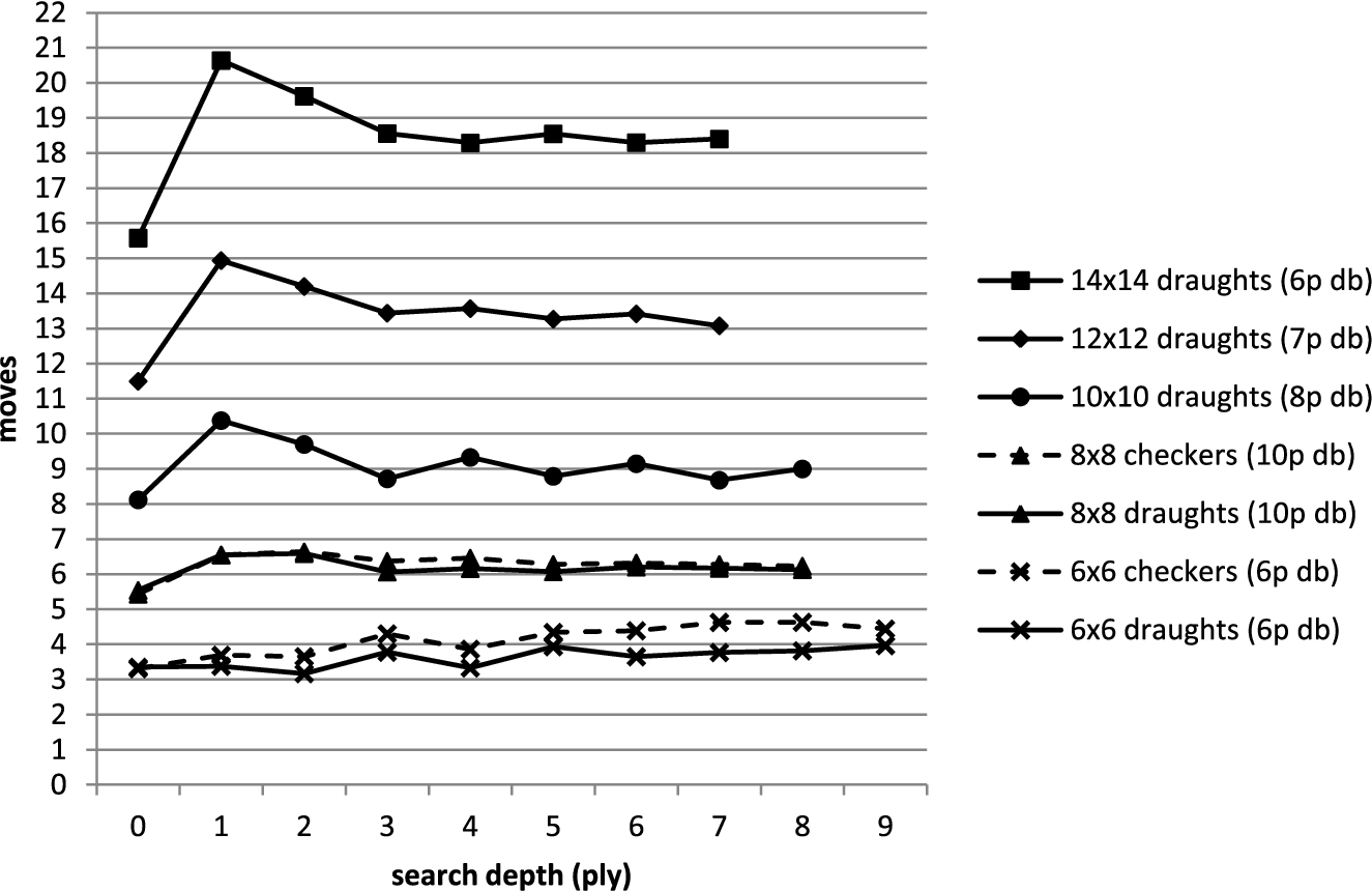For 10 × 10 draughts this means that a good lower bound for the GTC probably lies between $10^{92}$ (human database) and $10^{104}$ (our experiment).

Fig. 2.

Branching factor. Each data point represents max. 10,000 unique games.

Fig. 3.

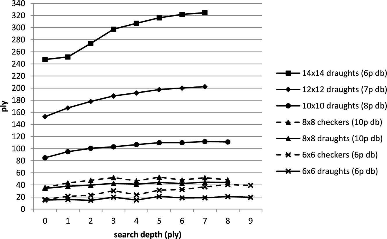
Average game length. Each data point represents max. 10,000 unique games.

Table 3

Experimental game-tree complexity

Game	Stop at # pieces	$b^{d}$	GTC ⩾
6 × 6 draughts	6	3.75¹⁹	8.1·10¹⁰
6 × 6 checkers	6	4.37³⁸	2.2·10²⁴
8 × 8 draughts	10	6.13⁴³	7.3·10³³
8 × 8 checkers	10	6.32⁴⁹	1.7·10³⁹
10 × 10 draughts	8	8.95¹¹⁰	5.0·10¹⁰⁴
12 × 12 draughts	7	13.36²⁰⁰	1.4·10²²⁵
14 × 14 draughts	6	18.42³²⁰	7.8·10⁴⁰⁴

4. Solving 6 × 6 checkers and 6 × 6 draughts

Subjects related to the complexity of a game are the possibility to solve the game and to achieve perfect play. For the small games 6 × 6 checkers and 6 × 6 draughts we can build endgame databases that cover a significant part of the state space. These can be used to weakly solve the games. Also, we reconsider the GTC of these games, using endgame databases of different sizes or no endgame database at all.

4.1. Weakly solving both games

The SSC of 6 × 6 checkers/draughts indicates that it is feasible to build the complete 12-piece databases for these games, that is, to strongly solve them. As this is still a considerable task, we decided to weakly solve the games, that is, to determine the game-theoretical value of the initial position. This was done by using a simplified version of the method used to solve 8 × 8 checkers (Schaeffer, 2007). To this end, we developed a high-performance engine for the 6 × 6 variants (named Hexamus, code derived from Maximus), using a bitboard data structure. This engine was also used to calculate the exact 6 × 6 SSCs in Section 2.

First, an endgame database was built, containing the win/draw/loss (WDL) result of all legal positions with 8 pieces or less ( $1.6 \times 10^{9}$ positions). Second, using this database, the game-theoretical value of the initial position was determined using proof-number search (PNS, see Allis, 1994), with repetition detection. To avoid the graph-history interaction (GHI) problem, no transposition table was used. The games are sufficiently small to afford this. Using the 8-piece databases, both games are proven a theoretical draw4

⁴
Both games were previously solved by Rein Halbersma (Halbersma, Online c), using alpha-beta and a transposition table but without using endgame databases. However, the GHI problem was ignored, so technically these are not conclusive proofs.

in a fraction of a second. It turns out that for 6 × 6 checkers using a 4-piece database is sufficient for a quick proof, and for 6 × 6 draughts even a 3-piece database. Using smaller databases or no database at all, no proof was found before running out of resources on a 64 GB RAM system. The results are shown in Tables 4 and 5. The most efficient computations of the game-theoretic values are the ones with the smallest database sufficient to find the proof.

Table 4

Data for solving 6 × 6 checkers with PNS and endgame databases

egdb (pieces)	egdb size (pos.)	Gen. egdb time (sec)	PNS nodes	PNS time (sec)	Max. depth	Avg. depth	Branching factor	Total time (sec)
8	1,617,366,257		37,718	0.07	21	9.2	3.1
7	322,389,233		163,789	0.17	34	12.1	3.0
6	48,881,249	819.92	466,345	0.26	35	13.4	3.0	820.18
5	5,789,784	61.94	7,544,866	3.62	51	21.7	3.2	65.56
4	512,910	6.00	35,547,846	17.49	61	25.9	3.3	23.49

Table 5

Data for solving 6 × 6 draughts with PNS and endgame databases

egdb (pieces)	egdb size (pos.)	Gen. egdb time (sec)	PNS nodes	PNS time (sec)	Max. depth	Avg. depth	Branching factor	Total time (sec)
8	1,617,366,257		101,297	0.11	20	10.6	3.0
7	322,389,233		298,718	0.23	29	13.1	3.0
6	48,881,249	986.52	816,974	0.46	38	15.2	3.0	986.99
5	5,789,784	106.79	2,307,446	1.08	39	16.8	2.9	107.87
4	512,910	6.67	6,057,396	2.45	42	18.5	2.9	9.12
3	31,155	0.54	15,986,551	6.68	54	23.0	3.1	7.22

4.2. Reconsidering game-tree complexity

In Section 3 we estimated the GTC of 6 × 6 checkers ( $2.2 \times 10^{24}$ ) and 6 × 6 draughts ( $8.1 \times 10^{10}$ ), a bit arbitrarily using (virtual) 6-piece databases. Combining alpha-beta search with distance-to-win (DTW) endgame databases, we can get better estimates for the “true” GTC of these games, using no endgame databases. For 6 × 6 checkers and 6 × 6 draughts, the 8-piece DTW databases were built (1.5 GB each; generating all databases together took about 100 CPU hours).

The longest win in the 6 × 6 checkers 8-piece database is 147 ply, with 68 consecutive king-slide moves. In a 6 × 6 checkers game, the first player has two losing first moves and three drawing first moves. Using alpha-beta search and the DTW database, the deepest first-player loss was established to be 66 ply away from the initial position. To find draws by repetition, even deeper searches will be needed (we did not introduce a rule that declares a game a draw after too many consecutive king moves without capturing). Thus the true GTC of 6 × 6 checkers is at least ${4.37}^{66} \approx 1.9 \times 10^{42}$ .

The longest win in the 6 × 6 draughts 8-piece database is 83 ply. In a 6 × 6 draughts game, all first-player moves are a draw, but the second player immediately has losing replies. Using alpha-beta search and the DTW database, the deepest second-player loss was established to be 61 ply away from the initial position. Thus the true GTC of 6 × 6 draughts is at least ${3.75}^{61} \approx 1.0 \times 10^{35}$ .

This shows the complexity of these games, even on such a small board. Of course, using endgame databases vastly reduces the GTC of a game.

4.3. Perfect play

Using the 8-piece DTW databases and PNS, a “perfect” player was created for both games. Perfect in the sense that, outside the database, it can almost always quickly determine the game-theoretic values of all moves, after which it randomly picks one of the best moves.5

⁵
In very rare cases it is not possible to determine the game-theoretic value of a move given the (modest) resource constraints of our player. So the result of a move can be unknown. If we have other moves that are winning or drawing we play one of those. If we don’t (other moves are losing or also unknown), we play a move with result unknown. It is assumed that this move is a draw by repetition that could not be proved with the given resources (max. number of iterations). Using this scheme, the player never lost a game.

The perfect player was paired against randomized alpha-beta players (using material evaluation with some fixed king value) to determine the search depth and database size combinations needed to never lose a game. Each test consisted of playing 12,000 games; passing the test requires all draws. For 6 × 6 checkers, a 14-ply search with an 8-piece database suffices. Using smaller databases revealed a deep opening trap where Black sacrifices a king, followed by a forced win in 57 ply. For 6 × 6 draughts, a 12-ply search with an 8-piece database suffices, or a 14-ply search with a 6-piece database, or a 17-ply search with a 4-piece database. It is not possible to extrapolate these results to the larger boards, since we have only one data point. We can, however, use these smaller games to do machine learning experiments, requiring less resources than would be needed for full-sized games. We can quickly generate large amounts of training data and test any learning algorithm objectively against a perfect player.

5. Conclusions

Below we provide five separate topical conclusions on (1) exponential and double exponential growth, (2) checkers rules versus draughts rules, (3) solved games, (4) statements on weakly solving, and (5) a comparison with chess and Go.

5.1. Exponential and double exponential growth

Figure 4 shows the complexity results found, compared to some popular games from literature (Allis, 1994; Schaeffer, 2007). The SSC of checkers and draughts grows exponentially with the board size; the GTC grows even double exponentially. This is mainly caused by the rapidly increasing game length. This means that checkers and draughts are games of deep strategy, also with increasing tactics when the board size increases. In our sample games, the maximum number of pieces captured in one move was 4 for 6 × 6 draughts, 6 for 8 × 8 draughts, 10 for 10 × 10 draughts, 12 for 12 × 12 draughts, and 17 for 14 × 14 draughts.

Fig. 4.

Game complexity of checkers and draughts from our experiments (left, middle) versus the complexity of some games from literature (right).

5.2. Checkers rules versus draughts rules

We have a strong indication that the rules of checkers make for a more complex game than the rules of draughts. This follows from our results concerning (1) the SSC, (2) the GTC, (3) the DTW endgame database, and (4) perfect play. Checkers is a “slower” but deeper game than draughts, also with a smaller draw margin.

5.3. Solved games

For 6 × 6 checkers and 6 × 6 draughts, the exact SSCs have been determined, as well as tight lower bounds for the GTC. Both games were also weakly solved; both are a theoretical draw. Strongly solving these games is feasible but this adds little, since perfect play can be achieved using the generated 8-piece DTW database combined with a short search.

The GTC and SSC of 8 × 8 checkers were previously determined and our results match those. The game of 8 × 8 checkers was weakly solved in 2007: Black to play and draw (Schaeffer, 2007).

5.4. Statements on weakly solving

For the game of 8 × 8 draughts, a first estimate for the GTC is given. This game is a candidate to be weakly solved, and it can be solved much faster than 8 × 8 checkers.

For 10 × 10 draughts, new estimates for the SSC and GTC are given. The GTC of 10 × 10 draughts is much higher than previously estimated: $10^{92}$ (human games) or $10^{104}$ (computer games) instead of $10^{54}$ (Allis, 1994). Regarding the GTC, the game is closer to chess than to checkers. Weakly solving draughts on a 10 × 10 board (or larger) is not feasible.

5.5. Comparison with chess and go

For 12 × 12 and 14 × 14 draughts, first estimates for the SSC and GTC are given. The GTC of 12 × 12 draughts exceeds that of chess. The GTC of 14 × 14 draughts exceeds that of Go. Both are due to a smaller branching factor but a far greater game length.

A higher GTC does not necessarily mean a game is more difficult. However, especially 14 × 14 draughts will be among the toughest games to master for computers. Methods that are known to be highly successful for 8 × 8 checkers and 10 × 10 draughts will start to break down: (1) alpha-beta search depth will be strategically insignificant compared to game length,6

⁶

A search in the opening will not reach middle game or even endgame positions, as is the case with the smaller games. This means that (opening) strategy depends more on evaluation and less on search. For instance, in 8 × 8 draughts we may search 20 ply deep in the opening, which is almost 50% of the average game length (43 ply), while in 14 × 14 draughts we may search 14 ply deep in the opening, which is less than 5% of the average game length (320 ply).

(2) evaluation becomes increasingly difficult to learn, (3) there is virtually no use for an opening book, and (4) the same goes for endgame databases. Applying an AlphaZero approach (Silver et al., 2017) seems obvious in this case. However, what sets draughts (and checkers) apart from the AlphaZero games (chess, shogi and Go) are the two rules (1) capturing is mandatory and (2) capturing multiple pieces in one move. This creates the possibility of deep forcing lines, posing a challenge to an MCTS-based search algorithm. A hybrid approach, combining the strengths of MCTS and alpha-beta search, has also been proposed, see, e.g., Lanctot et al. (2014) for positive results in the games of Kalah, Breakthrough and Lines of Action. Given the nature of combinations in draughts – long sequences of sacrifices, leaving the opponent (almost) no choice, completed by a winning capture and/or promotion – it is debatable whether the latter approach is useful in draughts. This is subject to future research.

Footnotes

Acknowledgements

Thanks to Rein Halbersma for pointing out an error in the initial calculation of the SSC of 14 × 14 draughts (caused by overflow) and for referring to Bik (). I thank Jaap van den Herik for proofreading. His comments are greatly appreciated. I also thank the anonymous referees for their helpful comments and suggestions.

Count depth-first with memory

Notes

Online publications retrieved 2018/05/10

References

Allis, L.V. (1994). Searching for Solutions in Games and Artificial Intelligence. Maastricht, The Netherlands: Rijksuniversiteit Limburg.

Fraenkel, A.S., Garey, M.R., Johnson, D.S., Schaefer, T. & Yesha, Y. (1978). The complexity of checkers on an n × n board. In 19th Annual Symposium on Foundations of Computer Science (pp. 55–64). IEEE. doi:10.1109/SFCS.1978.36.

Lanctot, M., Winands, M.H., Pepels, T. & Sturtevant, N.R. (2014). Monte Carlo tree search with heuristic evaluations using implicit minimax backups. Proceedings of the 2014 IEEE Conference on Computational Intelligence in Games (CIG) (pp. 1–8). IEEE.

Marsland, T.A. & Campbell, M. (1982). Parallel search of strongly ordered game trees. ACM Computing Surveys (CSUR), 14(4), 533–551. doi:10.1145/356893.356895.

Robson, J.M. (1984). N by N checkers is Exptime complete. SIAM Journal on Computing, 13(2), 252–267. doi:10.1137/0213018.

Schaeffer, J. (1983). The history heuristic. ICGA Journal, 6(3), 16–19. doi:10.3233/ICG-1983-6305.

Schaeffer, J. (2007). Game over: Black to play and draw in checkers. ICGA Journal, 30(4), 187–197. doi:10.3233/ICG-2007-30402.

Schaeffer, J. & Lake, R. (1996). Solving the game of checkers. Games of No Chance, 29, 119–133.

Silver, D., Hubert, T., Schrittwieser, J., Antonoglou, I., Lai, M., Guez, A. & Lillicrap, T. (2017). Mastering Chess and Shogi by Self-Play with a General Reinforcement Learning Algorithm. Arxiv preprint. Available at arXiv:1712.01815.

10.

Slate, D.J. & Atkin, L.R. (1977). Chess 4.5 – The Northwestern University Chess Program. In

P.W.

Frey (Ed.), Chess Skill in Man and Machine (pp. 82–118). Springer.

11.

Van Horssen, J.J. (2012). Schwarzman vs. MAXIMUS: A man-machine match in international draughts. ICGA Journal, 35(2), 106–119. doi:10.3233/ICG-2012-35209.

12.

Van Rijn, J.N. (2011). PSPACE-Hardness of Checkers and Draughts. Leiden, The Netherlands: Leiden Institute of Advanced Computer Science, Universiteit Leiden.

13.

Bik, A. (Online). Perft for 8 × 8 checkers. TalkChess. http://talkchess.com/forum3/viewtopic.php?topic_view=threads&p=680216&t=27814.

14.

Bor, K. (Online). Turbo Dambase. http://www.turbodambase.nl/tdamhome.php.

15.

Gilbert, E. (Online). Perft. World Draughts Forum. http://laatste.info/bb3/viewtopic.php?f=53&t=2308.

16.

Halbersma, R. (Online a). Perft for arbitrary board sizes. World Draughts Forum. http://laatste.info/bb3/viewtopic.php?f=53&t=2666.

17.

Halbersma, R. (Online b). Perft on large boards. World Draughts Forum. http://laatste.info/bb3/viewtopic.php?f=53&t=4563.

18.

Halbersma, R. (Online c). Search Algorithm. World Draughts Forum. http://www.laatste.info/bb3/viewtopic.php?f=53&t=4013&start=698.

19.

Van Horssen, J.J. (Online). Complexity of Checkers and Draughts on board sizes 6 × 6/8 × 8/10 × 10/12 × 12/14 × 14. World Draughts Forum. http://laatste.info/bb3/viewtopic.php?f=53&t=7817.

20.

Wikipedia (Online a). English draughts (or checkers), https://en.wikipedia.org/wiki/English_draughts.

21.

Wikipedia (Online b). International draughts, https://en.wikipedia.org/wiki/International_draughts.

22.

Wikipedia (Online c). Game complexity, https://en.wikipedia.org/wiki/Game_complexity.