Scalable data-driven modeling of spatio-temporal systems: Weather forecasting

Abstract

In this paper, a new data-driven method for short-range forecasting of spatio-temporal systems is proposed. It uses NCEP data as raw data to construct forecasting model. The global model consists of several local models. Each local model is constructed in three steps. In the first step, a local dataset is constructed based on NCEP raw data. This dataset is a very high-dimensional data with huge number of redundant and irrelevant features. In the second step, a feature selection method named GRASP is applied on the local dataset and produces a new local dataset whose features are reduced significantly. In the third step, a regression ensemble method called Bagging is used to construct a local model. Both GRASP and Bagging methods are scalable modules with respect to the computational power needed. The proposed method makes it possible to control the trade-off between speed and precision. In addition to the scalability, the proposed method, in some points produces forecasts more precise than the GFS system.

Keywords

Feature selection regression ensemble spatio-temporal modeling data driven modeling Numerical Weather Prediction

1. Introduction

Weather and climate forecasting are two applications of spatio-temporal modeling that have been the focus of much research in recent decades. Meteorological models have proved sufficiently accurate to be used in saving lives from disasters, as well as in strategic planning and management in agriculture. Nowadays, numerical models are the centerpiece of weather forecasting. However, in some aspects they have limitations that make it imperative to devise and examine alternative approaches. The two main limitations of numerical models are the dependency on domain knowledge of real system and low extendibility. Numerical models are completely dependent on the knowledge that describes the target system usually by differential equations. Extension of the numerical models is a difficult task since it requires a deep knowledge of the system. In this paper, a flexible and scalable method is proposed that can be used to model a wide range of spatio-temporal systems. Further, experiments are designed to prove the efficiency of the method in application to weather data, though there is no assertion on its generalization. This paper is focused on modeling of a spatio-temporal, complex and very high dimensional nonlinear system, i.e., the weather system. In weather forecasting, it is necessary to model the physics of the atmosphere. Constructing a perfect model for the complex system is too idealistic, so the main objective of all research in the field of weather forecasting is to construct useful and applicable models. Currently, irrespective of their deficiencies, the numerical models are certainly useful for the real-world applications.

Many real-world applications involve parameters that vary over space and time. In recent years, much research has been carried out on the study, analysis and forecast of spatio-temporal systems. Nowadays, spatio-temporal data are available in many areas, e.g. wind speeds and directions [42], rainfall [16, 49, 52], flood [29, 47], cloud-aerosol interaction [8], risk of agricultural crop disease [4], house prices [14, 28, 38], air pollution [19, 40, 46], brain imaging [1, 3, 13], wildlife population monitoring and tracking [33, 37], and machine vision [11, 24]. Spatio-temporal data analysis is aimed at predicting the system state in different locations at a time in the future. For spatio-temporal systems, the observed data consist of a large number of variables that vary over time and space. Recording the observed data may lead to a very large dataset. In spatio-temporal modeling, machine learning is used for the following three purposes:

1) 1)
Pre-processing of the data, e.g., dimension reduction, data interpolation and noise reduction;
2)
Extraction of the spatio-temporal system dynamics and its modeling;
3)
Estimation of the spatio-temporal system parameter values.

There are two main approaches in modeling spatio-temporal environmental phenomena such as those involved in hydrology and meteorology: 1-data-driven modeling, and 2-knowledge-driven modeling or physically-based modeling. In physically-based modeling, the real system or process is described by mathematical equations [7, 32, 35, 36, 41]. In fact, these equations are derived from the domain knowledge acquired from the natural phenomena. Physically-based modeling can also be divided into two categories: mathematical and numerical modeling. In case of mathematical modeling, mathematical equations are used to directly forecast the next state. Mathematical description occasionally consists of some partial differential equations that are analytically intractable. In this case, numerical techniques are used to approximate the future state.

Physically-based models can be constructed only if there is enough knowledge available about the natural phenomena. Here, modeling of the natural process or system is possible only if the history of main variables is available, and if the data can present the input-output relationships associated with the process or system. In such cases, the data-driven modeling (DDM) can be used to both model the process and forecast its future state [1, 2, 15, 22, 25, 27]. Recorded history of spatio-temporal systems may become a very large dataset describing several parameters that are extended in time and space. Appropriate modeling tools are needed to handle error, uncertainty, high volume of data, and achieve high degree of accuracy in spatio-temporal systems. Such tools are used for two main purposes: accurate forecast of the state of the system and interpolation of parameter values over the spatial region of interest. These tools should be able to work with large and complex datasets.

Big Data (BD) refers to high volume of data beyond the processing capabilities of usual computers. It is a term used to refer to a collection of large and complex data that is difficult to process using traditional methods and tools. Gartner Inc. [23] defines this term as:

“Big Data, is defined by three V’s as high volume, velocity, and variety information assets that demand cost-effective, innovative forms of information processing for enhanced insight and decision making.”

Variety refers to combination of different types of simple or complex, structured or unstructured data, e.g., transaction-level, user interaction, video, audio and text data. Facebook’s data is a good example for BD with very high degree of variety. Velocity is an indication of how quickly data can be available for the analysis. In a dynamic system, model should be updated once a significant change occurs in the system. Ignoring parts of the data carelessly, may lead to unacceptable or poor solutions. Larger data provides better analysis and better analysis results in higher confidence in decision making, more profit and less cost and risk. According to these definitions, weather data can be assumed to be BD. Weather data is a kind of BD because of its huge volume, increasing growth and variety of its parameters and spatial scattering. Each day, a huge number of weather and climate parameters in numerous locations are recorded and stored [4, 45, 57]. Volume of these data is huge, and their variety and generation velocity are high.

Clouds, precipitation, atmospheric gasses such as water vapor and the earth and the ocean surfaces are considered meteorological objects. Using absorbed, scattered or emitted electromagnetic radiation, remote sensing techniques are used to collect information from the meteorological objects. The first civilian application of remote sensing satellite technology, a weather satellite named TIROS-1 (Television and Infrared Observation Satellite – 1), was used to monitor and forecast weather conditions. High spatial and temporal resolution of the remotely-sensed imageries makes them a better alternative to the data obtained from synoptic stations. They can provide information about the Earth’s surface, different layers of atmosphere, and oceans. This information includes atmospheric moisture, humidity, cloud cover, snow and ice cover, sea temperatures, surface radiation, fog intensity, precipitation quantity and other meteorological parameters. This information can be utilized in Numerical Weather Prediction (NWP) models for weather forecasting. NWP models are fed with assimilated version of the aforementioned information. NWP models use data assimilation to estimate initial conditions by (i) reducing observation error due to using related and redundant observations and (ii) interpolating parameters in uncovered areas to produce uniformly distributed observations.
1.1 Different categories of weather and climate forecasting

According to the definitions provided by the World Meteorological Organization (WMO) [55], forecasting is performed within seven different time ranges. These time ranges are presented in Table 1.

Table 1
WMO standard forecasting ranges [55]

Forecast Type	Range	More descriptions
Nowcasting	Now to 2 hours
Very short range forecasting	2 hours up to 12 hours
Short range forecasting	12 hours up to 72 hours
Medium range forecasting	72 hours up to 10 days
Extended range forecasting	10 days up to 30 days	Forecast is usually averaged and expressed as a departure from climate values for that period.
Long range forecasting	30 days up to 2 years	Forecast can be divided into 3 sub-ranges: 1. Monthly outlook: Description of averaged weather parameters expressed as a departure (deviation, variation, anomaly) from climate values for that month (not necessarily the following month). 2. Three months or 90 days outlook: Description of averaged weather parameters expressed as a departure from climate values for that 90 days period (not necessarily the following 90 days period). 3. Seasonal outlook: Description of averaged weather parameters expressed as a departure from climate values for that season.
Climate forecasting	Beyond 2 years	• Climate variability prediction: Description of the expected climate parameters associated with the variation of inter-annual, decadal and multi-decadal climate anomalies. • Climate prediction: Description of expected future climate including the effects of both natural and human influences.

The reported work is focused on design and development of a scalable framework for very short range weather forecasting. In this paper, scalability of a method means that it is capable of controlling the computational power required to execute the model. The proposed method can construct more accurate models at the expense of more computational power. This framework is not limited to a specific system and can be used to forecast a wide range of spatio-temporal systems. This feature is due to some novelties in the proposed framework. First, it constructs a local model for each data point. Therefore, the number of parameters, the density of parameters in local neighborhoods and the variety of dynamics in different parts of the system cannot hinder the framework from forecasting the overall state of the system. Second, using scalable modules make the proposed method computationally scalable.

Section 2 describes some related works in data-driven weather forecasting. Sections 3 and 4 are brief reviews on feature selection in high-dimensional data and regression ensemble. The proposed method is introduced in Section 5. Section 6 presents the implementation results of the proposed method and their analysis. Finally, Section 7 contains concluding remarks.

2. Related works

Recent advances in physically-based weather forecast models together with precise parameter measurements and higher resolutions in both temporal and spatial domains have led to ever-increasing improvements in weather forecasts. These advances make physically-based models applicable to real-world forecasting problems. In the past decade, European Centre for Medium-Range Weather Forecasts (ECMWF) [7, 41, 51, 54] and the National Centers for Environmental Predictions (NCEP) [12, 31, 48] have provided numerical weather forecasting systems which are used throughout the word.

Without directly taking into account the underlying physical knowledge about the target system, data driven models rely solely on previous recorded history of the system. However, inaccuracy in data-driven modeling is inevitable. This inaccuracy is due to the simplification assumptions, insufficient training data, lack of model variables and model selection and configuration details. Most data-driven models are constructed using machine learning methods. In the reported works, data-driven modeling is used for two reasons.

The first reason is due to the fact that some existing spatio-temporal systems already have physically-based models but these models are not accurate or they are sometimes overly expensive. In these cases, data-driven models are used as an alternative for increasing accuracy or reducing cost. Fernando et al. [19] proposed a stochastic method for air quality prediction based on Neural Networks (NN) as an alternative for the commonly used deterministic photochemical air quality models. Their results show better performance for the NN in speed and cost without compromising the accuracy of predictions. Filippo et al. [21] used NN to predict sea level. One of the main challenges in their work was to handle gaps in the data where physically-based models are not capable of handling them. They used Fast Fourier Transform (FFT) to reconstruct the data. Their results are less accurate but comparable to results of an alternative method.

The second reason for using data-driven models is lack of enough knowledge about the dynamics of the system to construct such physically-based models. In these cases, a deep knowledge of the target system is lacking. However, there is sufficient data available to model the system by data-driven approach. Chang and Chien [9] used NN with multi-trend transfer function to forecast typhoon wave height near Taiwan. They used seven different variables in seven time lags, i.e., $t-4,t-8,t-12,\ldots,t-24$ . Their NN consists of two hidden layers and uses multiple transfer functions for different types of variables. Valverde et al. [50] used NNs for rainfall forecast in Sao Paulo region. They used several meteorological variables from ETA model as inputs. Quantity of rainfall in next time step is the output of their feed forward network. They compared NN against Multiple Linear Regression (MLR) and concluded that NN outperforms MLR. Wei and Watkins [53] investigated tree structured models to predict seasonal stream flow of Colorado river system. They used a logistic regression tree as predictor and several large-scale climate indices such as El Nino Southern Oscillation (ENSO) and Pacific Decadal Oscillation (PDO) as its inputs. Their results show that regression tree is capable of nonlinear input-output mapping. None of the data-driven research works on weather forecasting has considered the challenging problem of high-dimensionality in data of global forecasting. Forecasting rainfall, stream flow, wave height and air quality use a controllable number of parameters, however, this work considers the ultimate challenge of global forecasting. In some of the experimental results in this paper, the number of parameters exceeds 20000. Also, the most of similar researches are focused on forecasting a limited number of weather parameters (like rainfall) in a specific area (like a basin and specific coast). In these cases, the required computational power is manageable and this scalability is not an issue. The proposed method is capable of handling applications that require high computational power and can control the balance between the computational power needed and the accuracy of the results.

2.1 Feature selection in high dimensional data

Nowadays, many machine learning and pattern recognition problems deal with huge datasets. Hugeness of datasets implies using methods with lower time and space complexities. Dimension reduction is an option for reducing space complexity. Dimension reduction is the process of converting a dataset to a new one with lower dimensionality. Feature selection is a kind of dimension reduction that preserves the meaning of the features during the reduction process. Feature selection makes machine learning tasks faster, more understandable and sometimes even more accurate. In high-dimensional datasets, drawbacks of redundant and irrelevant features become even more critical. Judd [30] investigated modeling and forecasting of complex high dimensional nonlinear processes. The aim of Judd’s paper is to develop a scalable method that is capable of dealing with a very high-dimensional dataset of the kind encountered in weather forecasting. It uses a feature selection method that is based on an optimization method named Greedy Randomized Adaptive Search Procedure (GRASP). GRASP is a two-phase general optimization search algorithm introduced by Feo and Resende [17]. Extensions of this algorithm and its applications can be found in several subsequent works [18, 20, 39, 43]. Bermejo et al. [5] introduced a new algorithm for feature selection in high-dimensional data based on the GRASP meta-heuristic algorithm. This algorithm is depicted in Fig. 1.

Figure 1.

Pseudo code for feature selection based on GRASP meta-heuristic search algorithm [5].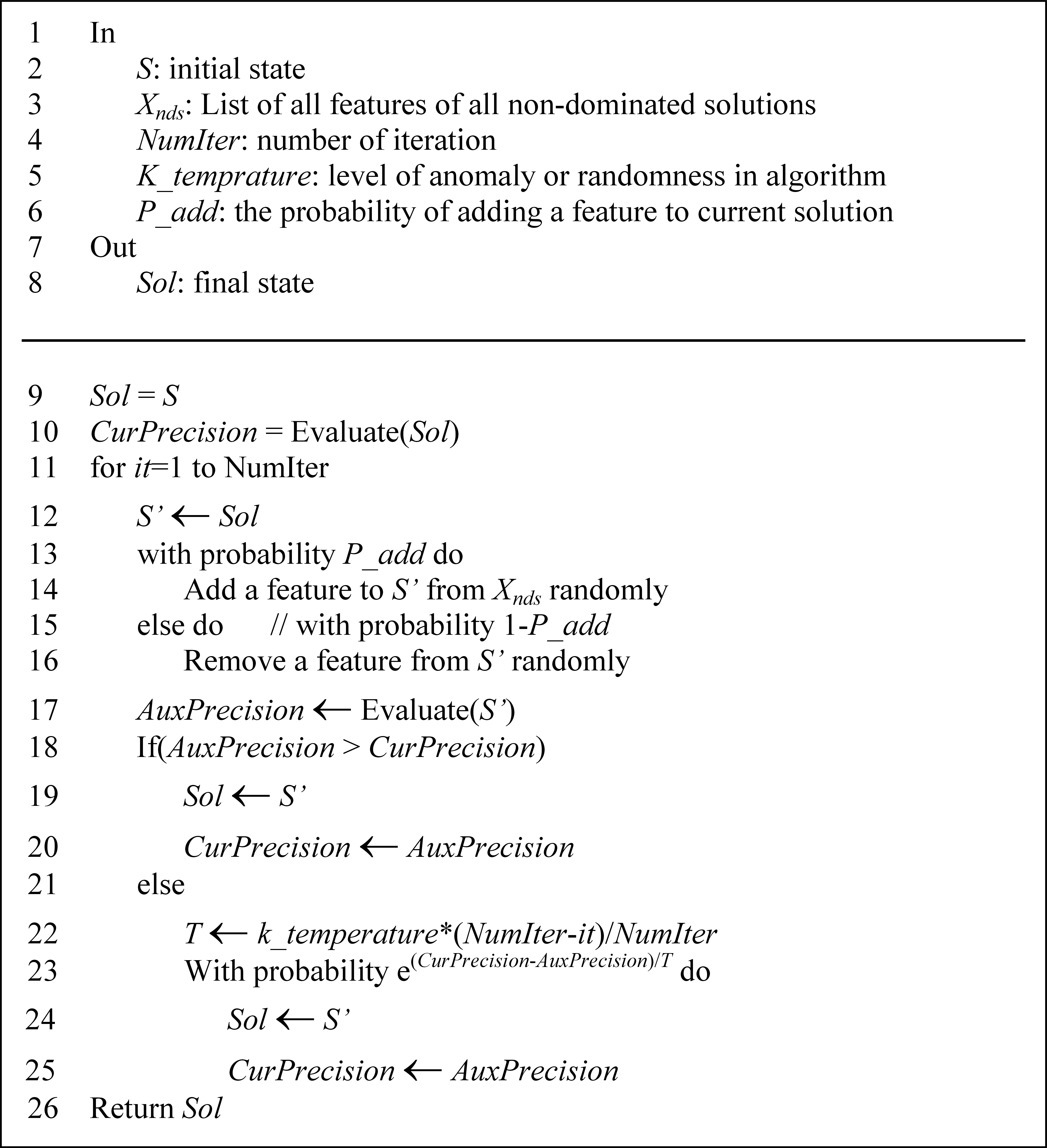

GRASP has two phases that execute iteratively: Phase 1-construction phase that starts with an empty set and enlarges set by randomly selecting items and, Phase 2-improvement phase that improves the output of construction phase using a local search algorithm. At the end of each iteration, both the constructed and the improved solutions are added to non-dominated solutions. A solution is called a dominated solution if there is at least one better solution with respect to accuracy and size of feature subsets.

2.2 Regression ensemble

Instead of a single learner, ensemble methods use multiple learners to produce a more accurate and complex learner [44]. The central idea behind the ensemble approach is to control the well-known trade-off between accuracy and complexity. Given a diverse set of learners, there is always a form of aggregation where an ensemble of learners may lead to a more accurate but more complex learner than each learner individually. Combining regressors, a more accurate ensemble is constructed at the expense of increased complexity. Ensemble methods are good options for using as an adjustable component to develop scalable frameworks. Using this component, Bagging is a simple but efficient solution to the problem of “how to build regressors for an ensemble” [6]. Bagging performs sampling with replacement to produce different subsets from the dataset. In Bagging, regressors are trained using the aforementioned subsets. There are a number of works reported on extension and improvement of this algorithm [10, 26, 34, 56].

3. The proposed method

The proposed framework has several characteristics that, when considered together, make it different from other spatio-temporal modeling frameworks:

•
It is scalable. In the proposed method, forecasting time can be reduced by compromising precision. Alternatively, precision can be improved at the expense of losing speed in forecasting.
•
Unlike NWP models, there is no need for a spatially homogeneous data. All NWP models need assimilated and gridded data. In the other words, NWP models have some spatial assumptions about the data but the proposed framework makes no such prior assumptions about the data. In the proposed method, data can be spatially heterogeneous.
•
In the NWP models data should be homogenous in term of the number of parameters in each cell. In the proposed method, each data point may have different number of parameters from the other points.
•
It can handle high dimensionality of some spatio-temporal systems that have large number of state parameters.
•
The proposed framework can be used to model any spatio-temporal system that is logged within a sufficiently longtime range. In other words, the only prerequisite for constructing model in the proposed framework is existence of rich history of system states.

Constructing scalable frameworks, it is necessary to control the well-known trade-off between precision and speed. Scalability provides a controllable trade-off between accuracy and speed. The main idea of this research is to use modules with adjustable control variables, i.e. feature selection and regression ensemble, for controlling this trade-off. Adjusting the modules is carried-out using two main scalability parameters in the proposed model: the number of features and the number of estimators. These parameters directly affect speed and precision of the model. Generally, increasing the number of features may lead to more precision at the expense of consuming more time. GRASP-based feature selection is a good option for selecting features since it is a multi-solution algorithm. As mentioned in Section 3, the output of GRASP-based algorithm is a set of feature subsets called Non-Dominated Solutions (NDS). These subsets may be different with respect to the number of features and resulting precision. Some definitions used in the proposed method are given in Table 2.

Table 2
Some definitions used in the proposed method

Weather history Includes all FNL files that show the state of the atmosphere within the 10-years period from 2000 to 2009. Weather history is used to construct local dataset.

Time step The time between two consequent representations of the atmosphere (two consequent FNL files).

Cell A cell $C_{x,y}$ refers to a cuboid volume with 1 $\times$ 1 degree area as base and a height proportional to the height of the atmosphere.

Cell data A cell data $D_{x,y}$ is the set of all variables in a cell. It includes several parameters in different atmospheric layers.

Local neighbourhood In this paper, local neighbourhood $N_{x,y}^{d}$ for a specific cell $C_{x,y}$ is a set of cells such as $C_{m,n}$ where $x-d\leqslant m\leqslant x+d$ and $y-d\leqslant n\leqslant y+d$ . For example, $N_{x,y}^{2}$ is a 5 $\times$ 5 square of cells centred by $C_{x,y}$ as illustrated in
Fig. 2.

Radius of dependency Radius of dependency $r$ is the radius of the region affecting a cell during a time step.

Local dataset A dataset consisting of a large number of input-output records that represent the relationship between all the parameters in $N_{x,y}^{r}$ as for inputs (or candidate features) and a specific parameter in that cell (target feature).

Reduced local dataset An edited version of local dataset only containing those features that can be useful in target feature prediction.

Local model The model that is trained on a reduced local dataset with the aim of forecasting a parameter based on all the correlated parameters.

Figure 2.
An example of local neighborhood with distance 2.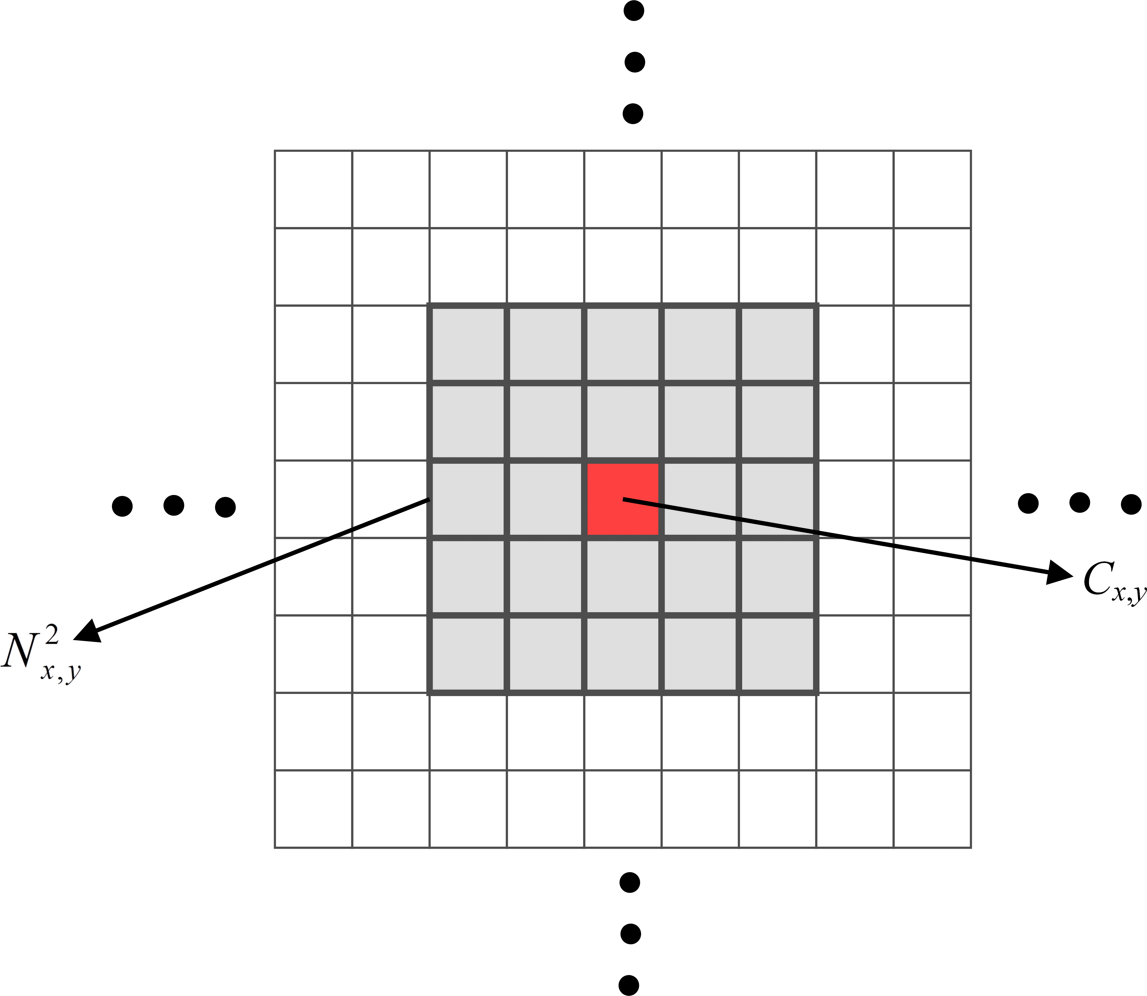

Weather forecasting is the same as predicting the next state of the atmosphere. Predicting the next state of the atmosphere requires determining the values of each parameter within each cell. To forecast the state of the whole atmosphere, a global model can be developed consisting of several local models. Each local model can be a black-box module predicting a target parameter for the next time step. This module maps values of all participating parameters in the neighborhood of the target cell to the value of the target parameter. The main focus of this paper is on developing a general framework for constructing these local models using machine learning and data mining techniques. More precisely, in the reported work each regressor represents a local model. Figure 3 shows the process of constructing the global model.

Once the region of interest is determined, a local model can be constructed for each parameter within the region. The role of each local model is to forecast its corresponding parameters for the next step. For each parameter in $C_{x,y}$ , a local model is constructed in the following three steps (Fig. 3):

•
Constructing a local dataset: A dataset should be constructed for each parameter. If the target parameter is within $C_{x,y}$ cell, the local dataset will consist of records such as $(\textbf{x},y)$ where x is a vector of all parameters in $N_{x,y}^{r}$ at time t and y is the target parameter at time t $+$ time step.
•
Applying the GRASP: Output from the previous step is a dataset with a very large number of features where the majority of them are redundant or irrelevant. Applying a feature selection algorithm to the dataset is necessary. GRASP is the proposed method for this process that converts the original the local dataset to a reduced local dataset.
•
Constructing local model: In this step, using the reduced local dataset, a local model is constructed. A regression ensemble module that implements Bagging algorithm is used to construct the local model.

Figure 3.
The process of constructing global model.

From a more practical point of view, there is large number of parameters that should be estimated. To estimate each parameter, all the aforementioned steps that are executed as demonstrated in the large rectangle depicted in Fig. 3. Initially, a local dataset is constructed from FNL files that includes two tables named $X$ and $Y$ . Table $X$ has $r$ rows and $f$ columns and table $Y$ has $r$ rows and one column. Number of rows in both tables is the same as the number of FNL files. Number of columns in table $X$ is equal to number of all the potentially effective parameters in neighborhood of the target parameter. Number of columns for each local dataset (more than 12000 parameters) is equal to the product of number of parameters in each cell (about 250 parameters), and number of neighbor cells for each target cell (49 cells in implementation). In the proposed method, GRASP is used to reduce the number of columns (candidate features). GRASP selects significantly smaller number of features (always less than hundred features). The final step in constructing a local model is to apply the Bagging method on the reduced local datasets that are filtered by GRASP. Bagging constructs an ensemble of regressor trees by which the conditional parameters selected by GRASP is mapped to the target parameter. Once construction of a local model is completed, it will be added to the local model pool and the construction process of the global model continues by constructing the next local model.

Executing the model, each local model is loaded and used to forecast a single parameter. All the forecasted parameters are used to form the next state of the atmosphere.
4. Introduction to the NCEP datasets

Weather history	Includes all FNL files that show the state of the atmosphere within the 10-years period from 2000 to 2009. Weather history is used to construct local dataset.
Time step	The time between two consequent representations of the atmosphere (two consequent FNL files).
Cell	A cell $C_{x,y}$ refers to a cuboid volume with 1 $\times$ 1 degree area as base and a height proportional to the height of the atmosphere.
Cell data	A cell data $D_{x,y}$ is the set of all variables in a cell. It includes several parameters in different atmospheric layers.
Local neighbourhood	In this paper, local neighbourhood $N_{x,y}^{d}$ for a specific cell $C_{x,y}$ is a set of cells such as $C_{m,n}$ where $x-d\leqslant m\leqslant x+d$ and $y-d\leqslant n\leqslant y+d$ . For example, $N_{x,y}^{2}$ is a 5 $\times$ 5 square of cells centred by $C_{x,y}$ as illustrated in Fig. 2.
Radius of dependency	Radius of dependency $r$ is the radius of the region affecting a cell during a time step.
Local dataset	A dataset consisting of a large number of input-output records that represent the relationship between all the parameters in $N_{x,y}^{r}$ as for inputs (or candidate features) and a specific parameter in that cell (target feature).
Reduced local dataset	An edited version of local dataset only containing those features that can be useful in target feature prediction.
Local model	The model that is trained on a reduced local dataset with the aim of forecasting a parameter based on all the correlated parameters.

National Centers for Environmental Prediction (NCEP) continuously produces several gridded datasets describing state of the atmosphere [50]. In this section, two types of NCEP files are described that are used in the reported work as the raw input data. These types are (FiNal Analysis) FNL files and Global Forecast System (GFS) forecasts.

4.1 FNL data description

NCEP FNL files are generated every 6 hours on both 0.5 $\times$ 0.5 and 1 $\times$ 1 degree grids by Global Data Assimilation System (GDAS). There are analyses available for different atmospheric levels such as the surface boundary layer, some sigma levels and the tropopause. The parameters include surface pressure, sea level pressure, geopotential height, temperature, sea surface temperature, soil-related values, ice cover, relative humidity, $u$ - and $v$ -horizontal velocity components, vertical motion, vorticity and concentration of tropospheric ozone.

More precisely, each 1 $\times$ 1 degree resolution FNL file describes the whole state of the atmosphere with a 181 $\times$ 360 grid of cells. In each grid cell, there are at least about 250 parameters (in early FNL files this number was originally 246 and now it has exceeded 350 parameters) in different atmospheric levels with different types. Figure 4 shows the overall structure of an FNL file. Common parameters within all FNL files are listed in Table 3.

Table 3
Common parameters within all FNL files

Abv	Description	Abv	Description
HGT	Geopotential height	CIN	Convective inhibition
TMP	Temperature	PWAT	Precipitable water
UGRD	$u$ -component of wind	CWAT	Could water
VGRD	$v$ -component of wind	TOZNE	Total ozone
ABSV	Absolute vorticity	TCDC	Total could cover
03MR	Ozone mixing ratio	VWSH	Vertical speed shear
RH	Relative humidity	4LFTX	Best (4 layer) lifted index
VVEL	Vertical velocity	HPBL	Planetary boundary layer height
CLWMR	Cloud water mixing ratio	POT	Potential temperature
PRES	Pressure	LAND	Landcover (0 $=$ sea 1 $=$ land)
SOILW	Volumetric soil moisture content	ICEC	Ice cover
WEASD	Water equivalent of accumulate	PRMSL	Pressure reduced to mean sea level
SPFH	Specific humidity	5WAVH	5-wave geopotential height
LFTX	Surface lifted index	GPA	Geopotential height anomaly
CAPE	Convective available potential energy	5WAVA	5-wave geopotential height anomaly

In this research, the 1 $\times$ 1 gridded FNL files are used. Figure 4 shows the overall structure of a FNL file.

Figure 4.

Overall structure of a FNL files.

4.2 GFS output files

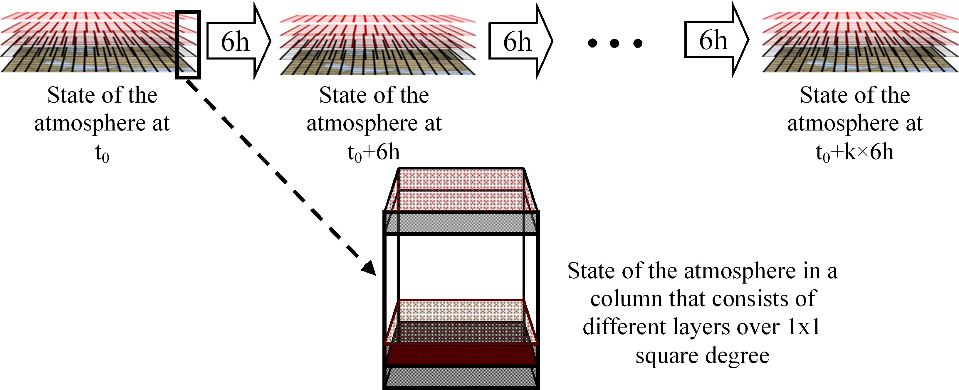
GFS is a Numerical Weather Prediction (NWP) model that consists of several components, i.e. an atmosphere model, an ocean model, a land model and a sea ice model. GFS is an evolving model due to improvements in hardware, data, algorithms and the underlying partial deferential equations solved numerically in the model.

This model runs every 6 hours and produces forecasts for more than 10 days. GFS uses FNL files for initialization and forecasting. In this paper, the term “GFS Data” refers to the output files produced by the GFS system.

4.3 The derived data

Forecasting weather means predicting the next state of the atmosphere. Predicting the next state of the atmosphere requires determining the values of each parameter within each cell. In the reported work, to forecast the whole state of atmosphere, a global model is developed that consists of several local models. Each local model can be a black box module predicting a target parameter in the next time-step. This module maps values of all participating parameters in a neighborhood of the target parameter to the value of the target parameter.

As mentioned before, each FNL file describes the whole state of the atmosphere by a 181 $\times$ 360 grid of cells. There are 65160 cells in this grid with different areas due to the spherical shape of the earth. As depicted in Fig. 5, each cell at latitude $x$ and longitude $y$ such as $C_{x,y}$ can be regarded as a semi-rectangular area with 8 neighbors. Due to the fact that the diameter of the earth is about 12742 kilometers, the maximum possible slice dimensions are around 110 kilometers.

Figure 5.

Eight neighbors of a cell.

Figure 6.

Generic local dataset with more details.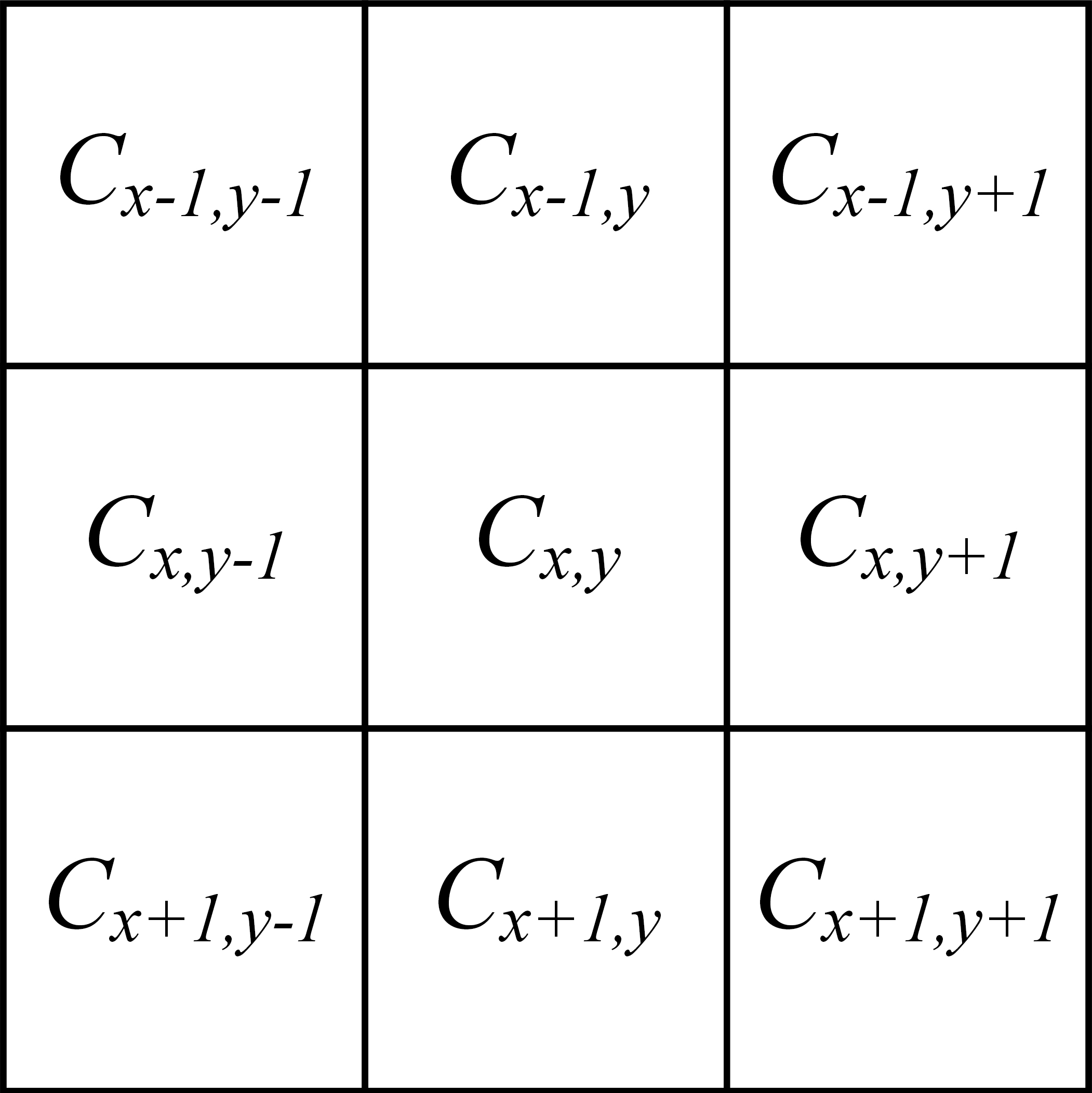

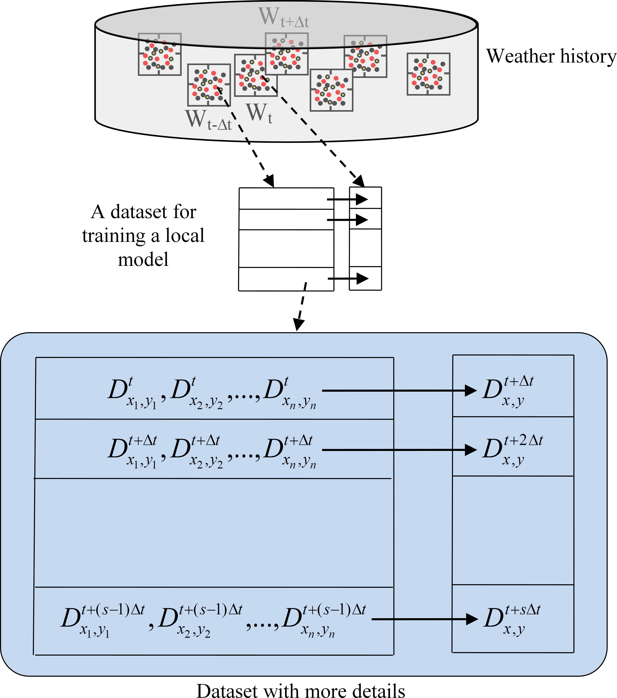
Each dataset consists of records, each mapping a set of parameters in a neighborhood of the target cell onto a parameter within the target cell. Let $\Delta t$ * be the longest time that a cell is affected only by its 8 adjacent cells. Radius of the neighborhood is called dependency radius $r$ and its value depends on the maximum propagation speed of atmospheric phenomena and processes. If $\Delta t$ is the time interval between two consequent records of the atmosphere, the dependency radius $r$ can be calculated using:

$r=\frac{\Delta t}{\Delta t^{\ast}}$ (1)

Construction of the dataset can be started only when r has been determined.

This paper is aimed at developing a general framework to construct these local models using machine learning and data mining techniques. More precisely, each regressor represents a local model. Training this regressor requires a dataset containing records in ordered pairs such as $(\textbf{x},y)$ , where x is a vector holding all the parameters that can potentially affect target parameter and $y$ is the value of the target parameter. Figure 6 shows a generic local dataset with more details. Weather history contains a large number of FNL files, each represents the overall state of the atmosphere within a specific time. In Fig. 6, $W_{t}$ represents an FNL file for time $t$ . The term $D_{x,y}^{t}$ includes all the parameters in a cell with longitude and latitude of, respectively, $x$ and $y$ at time $t$ and $\Delta t$ is the time step between FNL files. If $D_{x_{1c},y_{c}}^{t}$ represents all the parameters in the central cell, parameter sets $D_{x_{1},y_{1}}^{t}$ to $D_{x_{n},y_{n}}^{t}$ represent all the parameters within all the cells in the neighborhood. In another words, FNL files are used as the source of the raw data (weather history) to construct datasets for different cells. Each local dataset contains a large number of records. Each record determines both the state of the neighborhood of the central cell at time $t$ and the state of the central cell at the following time step, i.e., $t+\Delta t$ . Two FNL files are needed to construct each record of local dataset. $D_{x_{1},y_{1}}^{t},D_{x_{2},y_{2}}^{t},\ldots,D_{x_{n},y_{n}}^{t}$ is extracted from the first FNL file i.e., $W_{t}$ , and $D_{x_{c},y_{c}}^{t+\Delta t}$ is extracted from the second FNL file i.e., $W_{t}+\Delta t$ .

Determining what parameters in which neighborhood affect the target parameter is based on dynamical and/or thermodynamics considerations. In order to tune the $r$ parameter, several experiments have been performed the results of which are reported in Section 5.2. Since the sizes of the cells are predetermined, “the maximum propagation speed of the atmospheric processes” is the main question to be answered.

Table 4

Some of the most important parameters of regression tree in the reported experiments

Parameter	Description	Default value
Splitcriterion	Split selection criteria	Gini’s diversity index
Minparent	Impure nodes must have $k$ or more observations to split.	10
Minleaf	Minimal number of observations per tree leaf	1
Prune	Determines the full tree must be pruned or not	On

Figure 7.

Error map of the GFS system for the surface temperature field. In all pictures, i.e. the planar map and both spheres, pixels with hot colors are related to high error cells and those with cold colors are related to low error cells. Note that the sphere on the left side shows American continent and the one on the right shows asian continent.

5. Experimental results

In this section, three experiments are reported. The first experiment is a 6-hour forecast using the proposed method and results are compared against the results produced using the GFS. The second experiment is devoted to study the optimum value for the $r$ parameter. Finally, the third experiment demonstrates the scalability of feature selection and regression ensemble modules. In all the experiments, the NCEP data is used. All the regressors used in the reported work implement regression tree. Some of the most important parameters with their default values in the reported work and their descriptions are presented in Table 4.

5.1 Experiment 1: Comparing proposed method results against GFS

In this section, results produced by the proposed method are compared against the outputs of the GFS system for 6-hour forecasting. GFS system uses FNL files as input and produces forecasts as output files that have structures similar to FNL files. To compare results produced by the proposed method and the GFS system, first step is to extract their error maps for the surface temperature field. The error map of the GFS system is depicted in Fig. 7. Each point on the map shows the error of a cell within specific latitude and longitude. Hot pixels correspond to those points with high average errors and dark pixels correspond to points with low average error. For the temperature field, the minimum average error of GFS over all points is 0.02 in degrees Celsius and the maximum average error is 1.74 in degrees Celsius. In the reported work, only GFS error map is constructed. This was due to the fact that its forecasts and their corresponding ground truths were available. However, since construction of the complete global model was very time consuming, the proposed model was constructed for only the selected cells.

Table 5
Comparing the proposed method against the GFS system

Run number	Lat	Long	GFS error	# on features	No ensemble	Ens 10	Ens 50	Ens 100
1	40	45	0.47	13	2.18	1.56	1.53	1.54
2	37	38	0.39	12	2.53	1.82	1.73	1.73
3	31	44	0.21	33	2.14	1.43	1.35	1.32
4	28	33	0.59	17	1.71	1.29	1.23	1.23
5	28	35	0.68	23	1.46	1.06	0.99	1.00
6	28	50	0.65	8	0.83	0.61	0.57	0.57
7	26	56	0.73	9	1.05	0.77	0.74	0.74
8	20	46	0.11	12	1.57	1.31	1.26	1.25
9	20	54	0.10	18	1.68	1.26	1.20	1.20

Table 5 compares results produced by the proposed method against the outputs from the GFS system. Training local models is a time consuming task. Therefore, points with diverse GFS errors are selected for the comparison. Columns 2 and 3 of this table show latitude and longitude of the selected points with the error of GFS presented in Column 4. Column 5 shows the number of features selected by GRASP algorithm that is used as the feature selection module in the proposed method. Column 6 shows the error of the proposed method when a single regressor is used. Columns 7 to 9 show the error of the proposed method when ensembles with sizes of 10, 50 and 100 are used. Column 10 shows the distribution of the selected features in the neighborhood of the selected points. The value of $r$ parameter in all points is 3. Therefore, each picture in column 10 is in size 7 $\times$ 7 that shows spatial dependency of the cell to features in its neighborhood with $r=$ 3.

As seen in this table, in most points the error of the GFS is significantly lower than the proposed method (7 cells from all 9 cells). But in one cell with latitude of 28 and longitude of 50 the average error of the proposed method is lower than that of the GFS (see the row with run number 6), and in another one with latitude 26 and longitude 56 errors of the both methods are very close. At the first glance, it seems that the achievements of the proposed method are modestly less accurate compared to the GFS. However, there are several reasons for the usefulness and innovation of the proposed method. First, GFS is a mature system in the class of numerical weather prediction (NWP) systems, whereas the proposed method is an innovative, pioneering work in the category of data-driven methods and there is certainly room for improvement. Second, the quite different nature of the proposed method from NWP models makes it possible to combine it with systems like GFS in order to improve the results of NWP in short range forecasting at least in certain places. Third, the computation power needed in either of the NWP models is significantly larger than the proposed model.

5.2 Experiment 2: Studying the optimum size of r parameter

Finding the optimum value for $r$ is very important in the proposed method. It determines which cells can affect a target cell. Assigning a large value to $r$ may lead to large number of participating irrelevant parameters and assigning small values to $r$ may lead to missing some vital information. For example, when $r$ equals to 2, 3, 4 or 5 the number of cells become 25, 49, 81 or 121 respectively. At the same time, the number of parameters become 6050, 11858, 19602 or 29282, respectively. In this section, an experiment is designed to study the optimum value for $r$ parameter. Three suitable values for this parameter, i.e. 3, 4 and 5, are tested in this set of experiments. Table 6 shows the results.

Table 6
Comparing the results for different values of $r$ parameter

Cell number	Lat	Long	GFS error	# on features	No ensemble	Ens 10	Ens 50	Ens 100	r
1	28	50	0.65	8	0.83	0.61	0.57	0.57	3
			0.65	18	0.82	0.59	0.57	0.57	4
			0.65	11	0.85	0.63	0.61	0.60	5
2	28	35	0.68	23	1.46	1.06	0.99	1.00	3
			0.68	10	1.55	1.27	1.23	1.23	4
			0.68	25	1.47	1.03	0.99	0.97	5

As seen in Table 6, increasing the value of $r$ has no significant effect in improving the precision of forecasts. Increasing the value of $r$ has two main different effects. The positive effect is the higher normativity of including parameters. As an example, the error for the second cell with $r=$ 5 is slightly lower than the errors for $r=$ 3 and $r=$ 4. Considerable number of features for $r=$ 5 are not available in $r=$ 3 (see spatial dependency column for the second cell and for $r=$ 3 and $r=$ 5). From another point of view, increasing $r$ may lead to a vaster area and huge number of parameters. For example, the error for the second cell with $r=$ 4 is higher than the corresponding errors for $r=$ 3 and $r=$ 5. The reason of this discrepancy is the confusion of GRASP algorithm and disregarding some important features. For the second cell, the number of selected features for $r=$ 4 is less than half the number of features for $r=$ 3.

5.3 Experiment 3: Evaluating scalability of the proposed method

Scalability is one of the most important features of the proposed method. In this experiment, the scalability of the proposed method is evaluated. Scalable modules of the proposed methods are GRASP and regression ensemble modules. Therefore, the scalable ability of these modules is studied separately in this section.

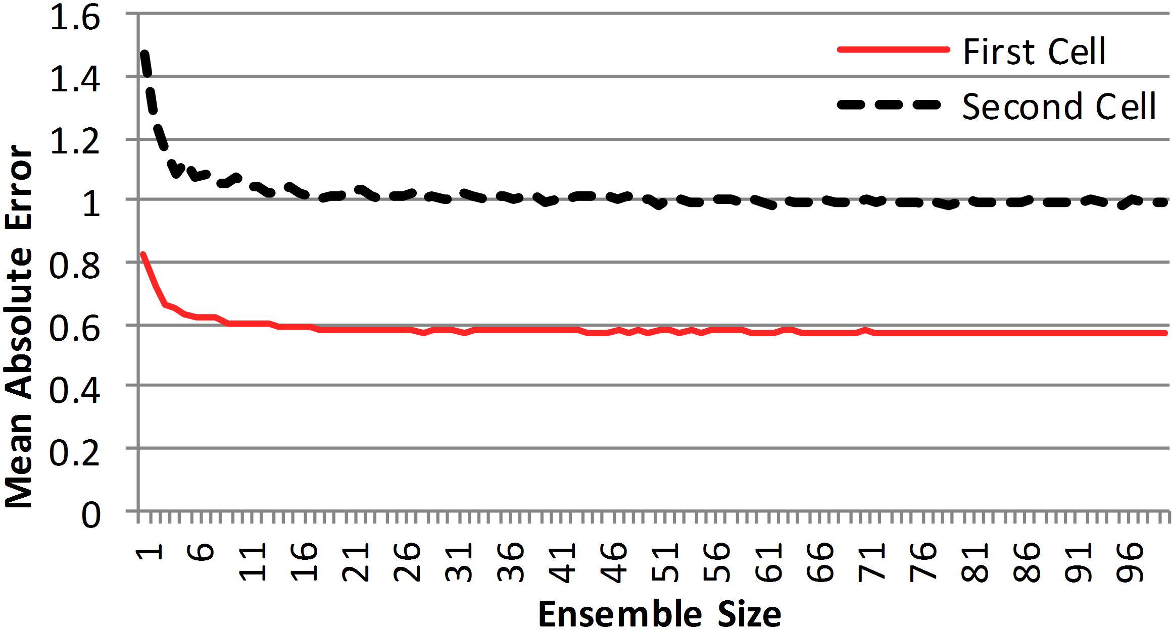
Regression ensemble module in the proposed method uses the Bagging algorithm. Size of ensemble is the controlling parameter of this module. By changing this parameter, one can control the trade-off between computation time and precision. Figure 8 shows the effect of mean absolute error of the ensemble against the size of the ensemble for two cells introduced in Section 5.2. As depicted in Fig. 8, for both cells the error of the Bagging decreases smoothly once ensemble size is increased.

There are two main important points in Fig. 8. First, the curves of error against ensemble size for both cells are smooth and predictable. Thus, it is possible to find suitable ensemble size to achieve a specific error. Second, Fig. 8 shows that there is no need to employ a large number of regressors in the ensemble. Error of the ensemble is almost constant for all ensemble sizes larger than 20. The second module, i.e. the feature selection, provides some degree of scalability but its effect is less than the regression ensemble module. Feature selection module works according to the GRASP algorithm which is a multi-solution method. GRASP always produces several feature subsets with different size and precision. Table 7 shows some details on the results of GRASP algorithm for two cells.

Table 7
Scalability of GRASP algorithm

Subset	First cell		Second cell
number	Number of	Error	Number of	Error
	selected		selected
	features		features
1	8	0.85	23	1.03
2	7	0.96	21	1.04
3	1	0.97	16	1.09
4	–	–	13	1.25

Figure 8.

Error of the proposed method versus different ensemble sizes.

For each cell, the number of the selected features and resulting error using corresponding feature subsets are reported in Table 7. For example, the output of GRASP for the second cell includes 4 feature subsets with sizes 23, 21, 16 and 13 and error values of 1.03, 1.04, 1.09 and 1.25, respectively. GRASP can be regarded as a semi-scalable method, since it is only partially controllable.

The scalability of the proposed method is best illustrated in results depicted in Figs 9 and 10. In Fig. 9, the forecast error of the proposed method is plotted against the ensemble size and the number of features (control parameters of regression ensemble and feature selection modules).

Figure 9.

Error of the proposed method plotted against different ensemble sizes and the number of features.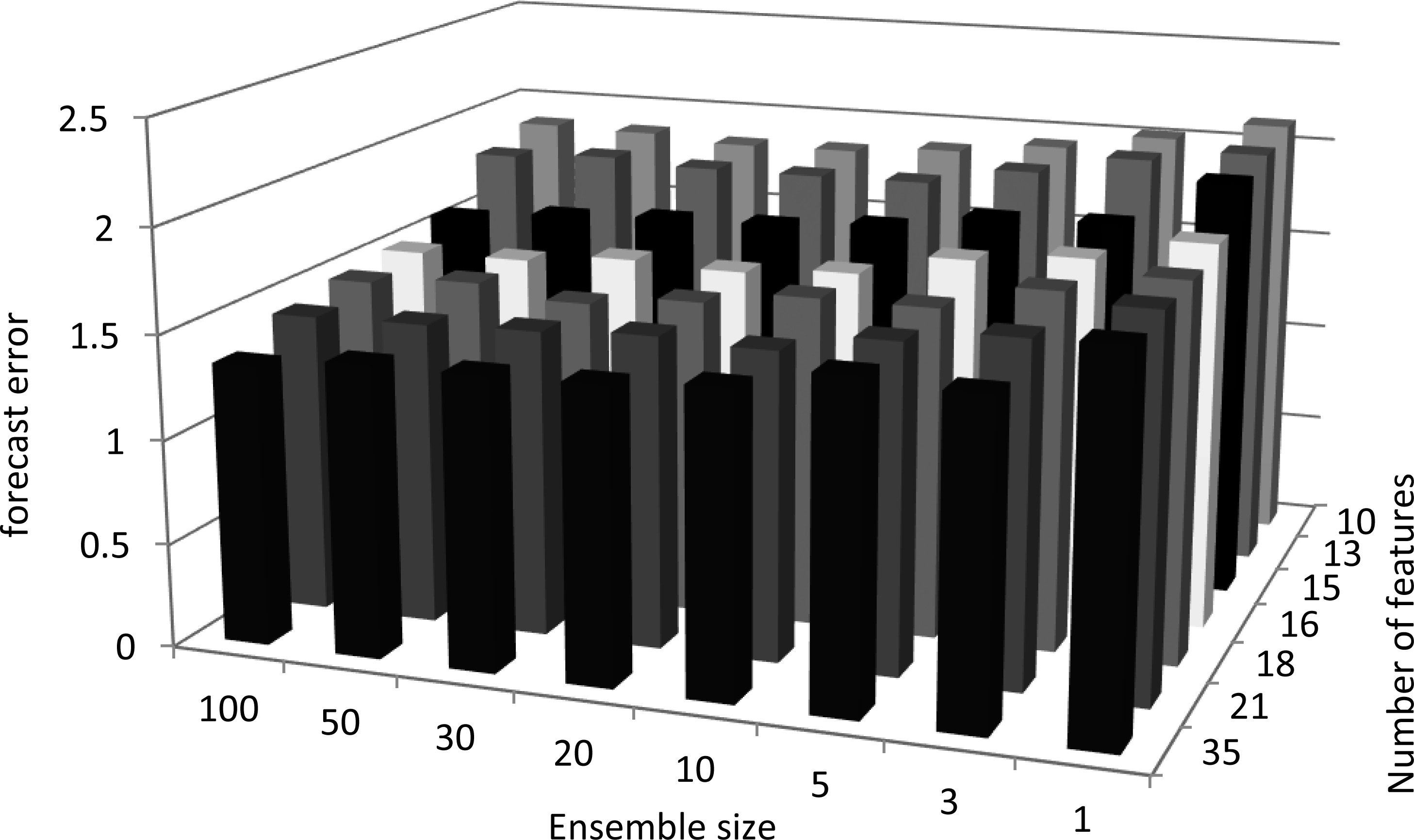

Further, In Fig. 10 the execution time of the proposed method for a period of one year is plotted against the ensemble size and the number of features.

Figure 10.

The execution time of the proposed forecast model for a period of one year is plotted against different ensemble sizes and the number of features.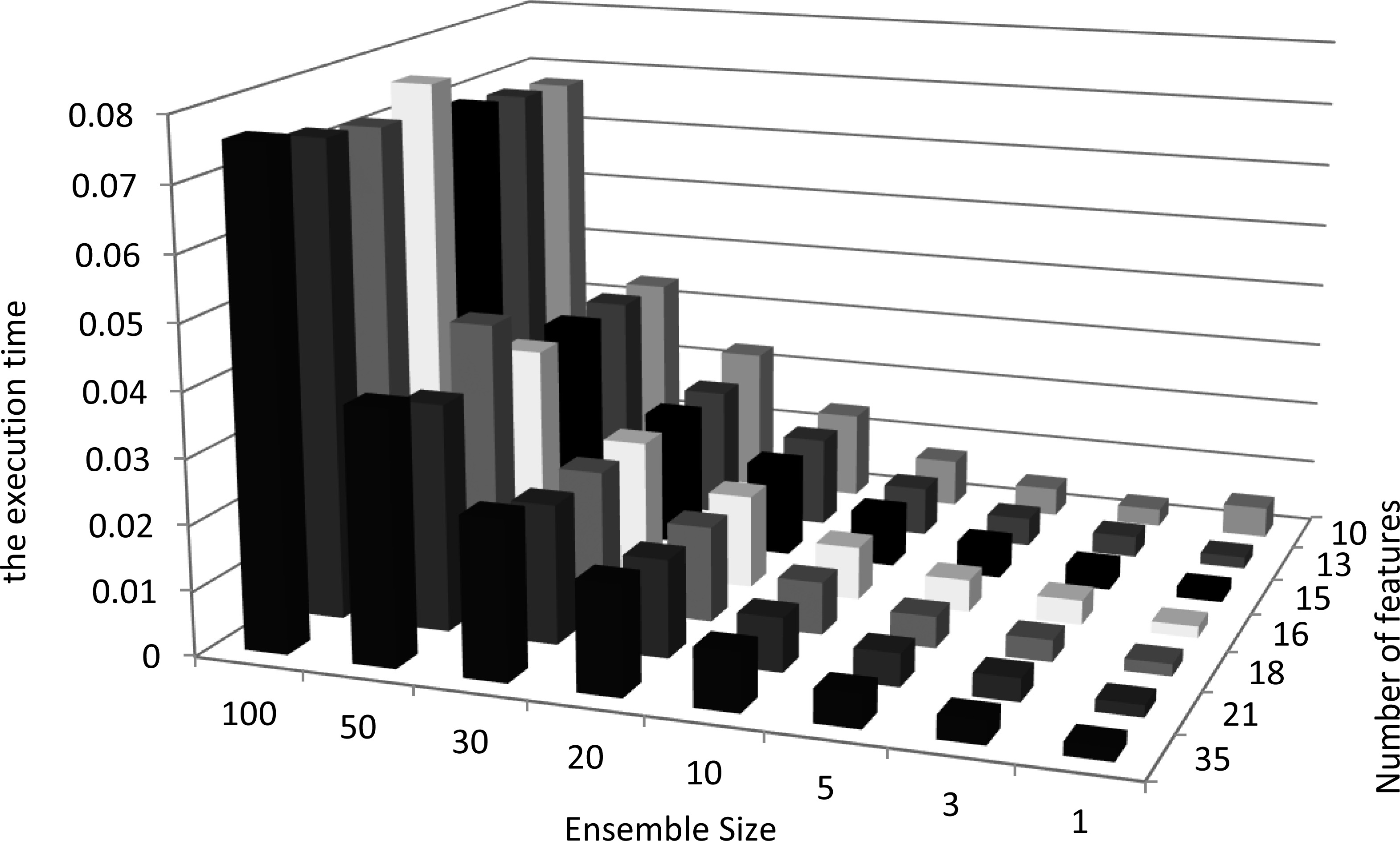

Figure 10 reports the time span for 1460 executions of the proposed model for a period of one year within 6 hours step i.e., 365 $*$ 4 executions. The reported time for the execution of the model is in seconds. The model is executed to estimate temperature of a cell within 45 degrees latitude and 40 degrees longitude within one year period. As depicted in Fig. 10, execution time is in direct and linear relationship with the ensemble size. Number of features is in direct relationship with execution time but its effect is negligible. The relationship between number of features and execution time is dependent on the type of regressor used in the ensemble. The number of features determines the number of inputs to the regressor. In some regressors such as Artificial Neural Network (ANN), number of inputs has significant effect on the required computational power. Number of inputs has negligible effect on the computational power needed in regression tree estimator. Examining the influence of ensemble size and number of selected features on the execution time of the global model, two-way ANOVA is applied to the results (Fig. 10). The $p$ -values for ensemble size and the number of selected features are calculated to be 0 and 0.0393 respectively. Calculated $p$ -values show strong effect of ensemble size and moderate effect of the number of selected features. For the forecasting error, $p$ -values are 3.2e-24 and 2.4e-30 for ensemble size and number of selected features respectively (both have strong effect of forecasting error).

Scalability and flexibility are two main privileges of the proposed method. The trade-off between speed and precision is selective and more controllable in the proposed method. The computational power needed in GFS and other NWP systems cannot be easily manipulated. The required execution power can be reduced only by reduction in spatial scale (grid resolution) and step size (time resolution). In the proposed method since each cell has its own model, it is possible to forecast different cells using different precisions. The proposed method can be applied to a wide range of application areas. It can model different spatio-temporal systems that have long and regular history. It should be noted that NWP method can model a system only if the analytical model of system is available in form of differential equations (white box approach).

6. Conclusion and future works

In this paper, a new data-driven method for short-range forecasting of spatio-temporal systems is proposed. It constructs forecasting model based on huge set of records from the target system. The paper is focused on weather forecasting and its spatio-temporal target system is the atmosphere. In all the reported experiments two types of data files from National Centers for Environmental Prediction (NCEP) are used i.e. FNL and GFS files. These datasets are used as raw data to construct datasets for local models. Each local model is a component of the global model that is used to forecast the next state of the atmosphere. Process of constructing local models is designed in such a way that the complexity of each local model is controllable. Using two scalable modules make it possible to control the trade-off between speed and precision. The relative stability of the error resulting from application of different feature and ensemble sizes that are directly linked to the execution time of the method, are presented to prove the scalability of the proposed method. Regression ensemble module is the first module that is fully scalable. The second is feature selection module which is semi-scalable. In addition to scalability of the proposed method, in some points it can even result in more accurate forecasts than the GFS system.

From theoretical point of view, as well as in its demonstrated application in weather forecasting, the proposed method can be used for forecasting purposes in other spatio-temporal systems. A large numbers of spatio-temporal systems exist all around the world whose state can be describe using large collection of data encompassing a long period of time.

Scalable modules in the proposed method have certainly potential for improvement. Making feature selection method fully scalable is an option for improvement. Also, feature selection and regression ensemble modules are independent. Proposing a way to interact these modules may improve the proposed method. The feature selection module may produce diverse feature subsets and these feature subsets can be used for constructing ensemble members.

References

Anastasio

T.J.

, Data-driven modeling of Alzheimer disease pathogenesis, J Theor Biol 290 (2011), 60–72.

Antoch

and Hlubinka

, Data driven modelling of vertical atmospheric radiation, J Environ Radioact 102 (2011), 1085–1095.

Badin

A.S.

Eraifej

and Greenfield

, High-resolution spatio-temporal bioactivity of a novel peptide revealed by optical imaging in rat orbitofrontal cortex in vitro: Possible implications for neurodegenerative diseases, Neuropharmacology 73 (2013), 10–18.

Baker

Lake

R.T.

Rivet

Benston

Bommersbach

and Kirk

, Point-trained models in a grid environment: Transforming a potato late blight risk forecast for use with the national digital forecast database, Computers and Electronics in Agriculture 105 (2014), 1–8.

Bermejo

Gámez

J.A.

and Puerta

J.M.

, A GRASP algorithm for fast hybrid (filter-wrapper) feature subset selection in high-dimensional datasets, Pattern Recognition Letters 32 (2011), 701–711.

Breiman

, Bagging predictors, Machine Learning 24 (1996), 123–140.

Buizza

Leutbecher

and Isaksen

, Potential use of an ensemble of analyses in the ECMWF ensemble prediction system, Quarterly Journal of the Royal Meteorological Society 134 (2008), 2051–2066.

Chakravarty

Mukhopadhyay

and Taraphdar

, Cloud microphysical properties as revealed by the CAIPEEX and satellite observations and evaluation of a cloud system resolving model simulation of contrasting large scale environments, Journal of Atmospheric and Solar-Terrestrial Physics 73 (2011), 1790–1797.

Chang

H.K.

and Chien

W.A.

, Neural network with multi-trend simulating transfer function for forecasting typhoon wave, Advances in Engineering Software 37 (2006), 184–194.

10.

Coelho

A.L.V.

and Nascimento

D.S.C.

, On the evolutionary design of heterogeneous Bagging models, Neurocomputing 73 (2010), 3319–3322.

11.

Cuevas

and García

, Improved background modeling for real-time spatio-temporal non-parametric moving object detection strategies, Image and Vision Computing 31 (2013), 616–630.

12.

Dash

and Ignatov

, Validation of clear-sky radiances over oceans simulated with MODTRAN4.2 and global NCEP GDAS fields against nighttime NOAA15–18 and MetOp-A AVHRR data, Remote Sensing of Environment 112 (2008), 3012–3029.

13.

Dong

Gong

Valdes-Sosa

P.A.

Xia

Luo

and Yao

, Simultaneous EEG-fMRI: Trial level spatio-temporal fusion for hierarchically reliable information discovery, Neuro Image 99 (2014), 28–41.

14.

Dubé

Thériault

and Des Rosiers

, Commuter rail accessibility and house values: The case of the montreal south shore, Canada, 1992–2009, Transportation Research Part A: Policy and Practice 54 (2013), 49–66.

15.

Everaert

Pauwels

I.S.

Boets

Buysschaert

and Goethals

P.L.M.

, Development and assessment of ecological models in the context of the european water framework directive: Key issues for trainers in data-driven modeling approaches, Ecological Informatics 17 (2013), 111–116.

16.

Awal

F.R.

Michaud

Chu

P.S.

Fares

Kodama

and Rosener

, Rainfall-runoff modeling in a flashy tropical watershed using the distributed HL-RDHM model, Journal of Hydrology (2014).

17.

Feo

T.A.

and Resende

M.G.C.

, A probabilistic heuristic for a computationally difficult set covering problem, Operations Research Letters 8 (1989), 67–71.

18.

Feo

T.A.

and Resende

M.G.C.

, Greedy randomized adaptive search procedures, Journal of Global Optimization 6 (1995).

19.

Fernando

H.J.

Mammarella

M.C.

Grandoni

Fedele

Di Marco

Dimitrova

and Hyde

, Forecasting PM10 in metropolitan areas: Efficacy of neural networks, Environ Pollut 163 (2012), 62–67.

20.

Festa

and Resende

M.G.C.

, Effective application of GRASP, Wiley Encyclopedia of Operations Research and Management Sciences 3 (2011), 1609–1617.

21.

Filippo Rebelo Torres

Kjerfve

and Monat

, Application of artificial neural network (ANN) to improve forecasting of sea level, Ocean & Coastal Management 55 (2012), 101–110.

22.

Friedel

M.J.

, Data-driven modeling of surface temperature anomaly and solar activity trends, Environmental Modelling & Software 37 (2012), 217–232.

23.

Gartner, What is big data, In: University of Villanova, 2012.

24.

Golparvar-Fard

Heydarian

and Niebles

J.C.

, Vision-based action recognition of earthmoving equipment using spatio-temporal features and support vector machine classifiers, Advanced Engineering Informatics 27 (2013), 652–663.

25.

Y.C.

Chan

P.W.

and Li

Q.S.

, Standardization of raw wind speed data under complex terrain conditions: A data-driven scheme, Journal of Wind Engineering and Industrial Aerodynamics 131 (2014), 12–30.

26.

Hernández-Lobato

Martínez-Muñoz

and Suárez

, Empirical analysis and evaluation of approximate techniques for pruning regression bagging ensembles, Neurocomputing 74 (2011), 2250–2264.

27.

Hill

D.J.

and Minsker

B.S.

, Anomaly detection in streaming environmental sensor data: A data-driven modeling approach, Environmental Modelling & Software 25 (2010), 1014–1022.

28.

Holly

Pesaran

M.H.

and Yamagata

, The spatial and temporal diffusion of house prices in the UK, Journal of Urban Economics 69 (2011), 2–23.

29.

Hsiao

L.F.

Yang

M.J.

Lee

C.S.

Kuo

H.C.

Shih

D.S.

Tsai

C.C.

Wang

C.J.

Chang

L.Y.

Chen

D.Y.C.

Feng

Hong

J.S.

Fong

C.T.

Chen

D.S.

Yeh

T.C.

Huang

C.Y.

Guo

W.D.

and Lin

G.F.

, Ensemble forecasting of typhoon rainfall and floods over a mountainous watershed in Taiwan, Journal of Hydrology 506 (2013), 55–68.

30.

Judd

, Forecasting with imperfect models, dynamically constrained inverse problems, and gradient descent algorithms, Physica D: Nonlinear Phenomena 237 (2008), 216–232.

31.

Koren

Smith

and Cui

, Physically-based modifications to the sacramento soil moisture accounting model, Part A: Modeling the effects of frozen ground on the runoff generation process, Journal of Hydrology (2014).

32.

Lang

S.T.K.

Leutbecher

and Jones

S.C.

, Impact of perturbation methods in the ECMWF ensemble prediction system on tropical cyclone forecasts, Quarterly Journal of the Royal Meteorological Society 138 (2012), 2030–2046.

33.

Lange

Siemen

Blome

and Thulke

H.H.

, Analysis of spatio-temporal patterns of African swine fever cases in Russian wild boar does not reveal an endemic situation, Preventive Veterinary Medicine (2014).

34.

Lin

Chen

Qiu

Krishnan

and Zou

, LibD3C: Ensemble classifiers with a clustering and dynamic selection strategy, Neurocomputing 123 (2014), 424–435.

35.

Mathiesen

Collier

and Kleissl

, A high-resolution, cloud-assimilating numerical weather prediction model for solar irradiance forecasting, Solar Energy 92 (2013), 47–61.

36.

Mathiesen

and Kleissl

, Evaluation of numerical weather prediction for intra-day solar forecasting in the continental United States, Solar Energy 85 (2011), 967–977.

37.

Milne

and Bennett

, Understanding landscape patterns of temporal variability in avian populations to improve environmental impact assessments, Ecological Informatics 14 (2013), 75–78.

38.

Moscone

Tosetti

and Canepa

, Real estate market and financial stability in US metropolitan areas: A dynamic model with spatial effects, Regional Science and Urban Economics 49 (2014), 129–146.

39.

Moshki

Kabiri

and Mohebalhojeh

, Scalable feature selection in high-dimensional data based on GRASP, Applied Artificial Intelligence 29 (2015), 283–296.

40.

Padilla

C.M.

Kihal-Talantikite

Vieira

V.M.

Rossello

Nir

G.L.

Zmirou-Navier

and Deguen

, Air quality and social deprivation in four French metropolitan areas – A localized spatio-temporal environmental inequality analysis, Environmental Research 134 (2014), 315–324.

41.

Pelly

J.L.

and Hoskins

B.J.

, How well does the ECMWF ensemble prediction system predict blocking? Quarterly Journal of the Royal Meteorological Society 129 (2003), 1683–1702.

42.

Rasheed

Sørli

Holdahl

and Kvamsdal

, A multiscale approach to micrositing of wind turbines, Energy Procedia 14 (2012), 1458–1463.

43.

Resende

M.G.C.

and Ribeiro

C.C.

, Greedy randomized adaptive search procedures: Advances, hybridizations, and applications, Handbook of Metaheuristics International Series in Operations Research & Management Science 146 (2010), 283–319.

44.

Rokach

, Ensemble-based classifiers, Artificial Intelligence Review 33 (2010), 1–39.

45.

Schnase

J.L.

Duffy

D.Q.

Tamkin

G.S.

Nadeau

Thompson

J.H.

Grieg

C.M.

McInerney

M.A.

and Webster

W.P.

, MERRA analytic services: Meeting the big data challenges of climate science through cloud-enabled climate analytics-as-a-service, Computers, Environment and Urban Systems (2014).

46.

Shaddick

and Zidek

J.V.

, A case study in preferential sampling: Long term monitoring of air pollution in the UK, Spatial Statistic 9 (2014), 51–65.

47.

Shih

D.S.

Chen

C.H.

and Yeh

G.T.

, Improving our understanding of flood forecasting using earlier hydro-meteorological intelligence, Journal of Hydrology 512 (2014), 470–481.

48.

Stopa

J.E.

and Cheung

K.F.

, Intercomparison of wind and wave data from the ECMWF reanalysis interim and the NCEP climate forecast system reanalysis, Ocean Modelling 75 (2014), 65–83.

49.

Valverde

M.C.

Araujo

and Campos Velho

, Neural network and fuzzy logic statistical downscaling of atmospheric circulation-type specific weather pattern for rainfall forecasting, Applied Soft Computing 22 (2014), 681–694.

50.

Valverde Ramírez

M.C.

de Campos Velho

H.F.

and Ferreira

N.J.

, Artificial neural network technique for rainfall forecasting applied to the São Paulo region, Journal of Hydrology 301 (2005), 146–162.

51.

Verkade

J.S.

Brown

J.D.

Reggiani

and Weerts

A.H.

, Post-processing ECMWF precipitation and temperature ensemble reforecasts for operational hydrologic forecasting at various spatial scales, Journal of Hydrology 501 (2013), 73–91.

52.

Villarini

Seo

B.C.

Serinaldi

and Krajewski

W.F.

, Spatial and temporal modeling of radar rainfall uncertainties, Atmospheric Research 135–136 (2014), 91–101.

53.

Wei

and Watkins

D.W.

, Data mining methods for hydroclimatic forecasting, Advances in Water Resources 34 (2011), 1390–1400.

54.

Wiegand

and Knippertz

, Equatorward breaking Rossby waves over the north atlantic and mediterranean region in the ECMWF operational ensemble prediction system, Quarterly Journal of the Royal Meteorological Society 140 (2014), 58–71.

55.

WMO, Definitions of meteorological forecasting ranges, in: WMO (2014).

56.

Xie

and Zhu

, Margin distribution based bagging pruning, Neurocomputing 85 (2012), 11–19.

57.

Zhang

Wang

and Wang

, Review on probabilistic forecasting of wind power generation, Renewable and Sustainable Energy Reviews 32 (2014), 255–270.

Scalable data-driven modeling of spatio-temporal systems: Weather forecasting

Abstract

Keywords

1. Introduction

Table 1 WMO standard forecasting ranges [55]

2.1 Feature selection in high dimensional data

3. The proposed method

4.1 FNL data description

Table 3 Common parameters within all FNL files

4.3 The derived data

5.1 Experiment 1: Comparing proposed method results against GFS

Table 5 Comparing the proposed method against the GFS system

Table 6 Comparing the results for different values of r parameter

Table 7 Scalability of GRASP algorithm

References

Table 1
WMO standard forecasting ranges [55]

Table 3
Common parameters within all FNL files

Table 5
Comparing the proposed method against the GFS system

Table 6
Comparing the results for different values of $r$ parameter

Table 7
Scalability of GRASP algorithm