Multi-label text classification based on the label correlation mixture model

Abstract

In the current paper, we propose a probabilistic generative model, the label correlation mixture model (LCMM), to depict multi-labeled document data, which can be utilized for multi-label text classification. LCMM assumes two stochastic generative processes, which correspond to two submodels: 1) a label correlation model; and 2) a label mixture model. The former model formulates labels’ generative process, in which a label correlation network is created to depict the dependency between labels. Moreover, we present an efficient inference algorithm for calculating the generative probability of a multi-label class. Furthermore, in order to optimize the label correlation network, we propose a parameter-learning algorithm based on gradient descent. The second submodel in the LCMM depicts the generative process of words in a document with the given labels. Different traditional mixture models can be adopted in this generative process, such as the mixture of language models, or topic models. In the multi-label classification stage, we propose a two-step strategy to most efficiently utilize the LCMM based on the framework of Bayes decision theory. We conduct extensive multi-label classification experiments on three standard text data sets. The experimental results show significant performance improvements comparing to existing approaches. For example, the improvements on accuracy and macro F-score measures in the OHSUMED data set achieve 28.3% and 37.0%, respectively. These performance enhancements demonstrate the effectiveness of the proposed models and solutions.

Keywords

Label correlation mixture model probabilistic generative model multi-label text classification label correlation model label correlation network Bayes decision theory

1. Introduction

Multi-label text classification represents a practical classification problem in the real world. For example, a financial news article may be classified not only under the “economy” class, but also under the “politics” class. Formally, consider D an observed document data set, and Y a label set with $K$ ( $K>1$ ) labels. The multi-label text classification problem concerns how to build optimal text classifier F based on a certain learning criterion:

$\displaystyle\textbf{F}:\textbf{d}\rightarrow\textbf{y}.\ \textbf{d}\in\textbf% {D},\textbf{y}\subseteq\textbf{Y}.$

where y is a subset of Y, which means that y is set-valued. This represents a more difficult text classification problem compared with the traditional classification task, in which one, and only one, label must be assigned to a document.

The existing multi-label classification approaches can be broadly grouped into two main categories [1, 2]: problem transformation methods and algorithm adaptation methods. Problem transformation methods, such as the classifier chain [3], label power-set [4], and maximal figure-of-merit [5, 6], transform the multi-label classification problem into one or more single-label classification problems. Algorithm adaptation methods modify and extend the existing algorithm to directly solve a multi-label problem. Typical algorithm adaptation methods include Boostexter [7], multi-label KNN [8], and multi-label neural networks [9].

According to the Bayes decision theory of minimum error rate case, given a new document $\textbf{d}^{\prime}$ , the goal of multi-label classification is to find the optimal label subset $\hat{\textbf{y}}$ , which maintains the maximum posterior probability. Every label subset is an independent multi-label class and should be assessed in theory. This approach can be regarded as a problem transformation method. According to the Bayes’ rule:

$\displaystyle\hat{\textbf{y}}=\operatorname*{argmax}_{\textbf{y}\subseteq% \textbf{Y}}P(\textbf{y}|\textbf{d}^{\prime})=\operatorname*{argmax}_{\textbf{y% }\subseteq\textbf{Y}}\frac{P(\textbf{d}^{\prime}|\textbf{y})P(\textbf{y})}{P(% \textbf{d}^{\prime})}=\operatorname*{argmax}_{\textbf{y}\subseteq\textbf{Y}}P(% \textbf{d}^{\prime}|\textbf{y})P(\textbf{y}).$ (1)

The key problem in this approach is how to build models to calculate the prior probability $P(\textbf{y})$ and the conditional probability $P(\textbf{d}^{\prime}|\textbf{y})$ . Generally, we appeal to the probabilistic generative model, which involves how to formulate the generative process of multi-labeled document data, including labels and words. Three essential questions should be addressed:

Q1.

How can the correlation between labels be formulated?

Q2.

How can the visible label subset information be formulated into the supervised learning procedure?

Q3.

How can all of the label subsets for a testing document be efficiently assessed?

In this paper, we propose a probabilistic generative model, named label correlation mixture model (LCMM) [10, 11] to answer the previous three questions, and emphasize that the LCMM presents not only a concrete model, but also a framework of generative modeling for multi-labeled document data. LCMM comprises two submodels: 1) a label correlation model; and 2) a label mixture model. The label correlation model formulates the generative process of labels of a document. A label correlation network models the dependency between labels, which addresses the first question, Q1. We present an efficient inference algorithm for calculating the prior probability of an arbitrary label subset, which is related to the third question, Q3. Furthermore, we propose a parameter-learning procedure in this paper to optimize the weights in the label correlation network. The label mixture model formulates the generative process of words in a document with a given label subset, which copes with the second question, Q2. This is a typical mixture model [12], in which words in a document are assigned to different mixture components associated with labels. Numerous traditional models can be chosen as the label mixture model. In the current paper, we select the LDA model, i.e. a full Bayesian model, to formulate words’ generative process in a document. In the multi-label classification stage, each multi-label class should be assessed according to Eq. (1) when a testing document is provided. However, the number of multi-label classes is an exponential function ( $2^{K}-1$ ) of $K$ , which means it may be impossible to assess every multi-label class, even when $K$ is not very large. This problem also relates to the third question, Q3, in response to which we propose a two-step strategy for establishing efficient classifications.

The remainder of this paper is organized as follows. Section 2 briefly reviews related studies. Section 3 presents the general form of LCMM. Section 4 describes the first submodel, the label correlation model, and then provides the inference and parameter learning algorithms for this model. Section 5 discusses the second submodel, the label mixture model, and its inference method. Section 6 provides the two-step strategy employed in the multi-label classification stage. Experimental results and discussion are presented in Section 7. Finally, Section 8 presents our conclusions.

Table 1

Definitions of notation

D	document data corpus
d	document
$M$	size of D
W	vocabulary
$V$	size of W
Y	the entire label set
$K$	size of Y
$\lambda$	multinomial parameters for the size of label subset
$\varphi$	multinomial parameters for sampling the first label
$\Xi$	parameters of label correlation network
y	label subset for a document
$L$	size of y
$y_{l}$	$l^{th}$ label in the label generative process
$N$	number of words in a document
$z_{n}$	label assignment of $n^{th}$ word in a document
$w_{n}$	$n^{th}$ word in a document
$\Phi_{\textbf{y}}$	all the possible orders of labels in y
$S_{L}$	$L$ labels of a document in a certain order
$\overline{\textbf{y}}$	complementary set of y
$\textbf{y}*$	candidate set of y
$y,y^{\prime},y^{\prime\prime}$	label variables
$\xi$	weight on the edge of the label correlation network
$\kappa$	conditional probability of selecting a label when
	a label subset is given
$A\setminus B$	set $B$ ’s complementary set when $A$ is given as the
	universal set

2. Related work

Due to the inherent ability to model document data in a generative way, we utilize the methodology of topic model to address the multi-label text classification problem in the framework of Bayes decision theory. The traditional topic models were proposed to model text and other discrete collective data, such as probabilistic latent semantic analysis (PLSA) [13], latent Dirichlet allocation (LDA) [14] and their variations, in which each word of a document is modeled as a mixture of a set of topics. However, since the parameters are learned in unsupervised ways, these models can not be directly employed for the multi-label text classification task.

Numerous supervised approaches of topic models have been proposed in recent years. A class mixture model approach was proposed in [15] for multi-label text classification, in which each label was regarded as a class and modeled by a word distribution. The model, utilized to calculate $P(\textbf{d}^{\prime}|\textbf{y})$ , resembled PLSA except for a slightly dissimilar method of updating parameters. However, the approach directly employed the frequency of a multi-label class to estimate its prior probability $P(\textbf{y})$ . This is inappropriate for many real applications, because sufficient data often fail to exist to estimate the priors of all the multi-label classes. Labeled LDA (L-LDA) was proposed in [16] as a direct way to train the parameters of the LDA model with supervised label information. Compared with the LDA model, L-LDA completes an additional Bernoulli sampling process to depict that only a label subset, rather than all the labels, associates with a document. One weakness of L-LDA is that the correlation between labels were not considered because of the Bernoulli sampling process. Additionally, the CoL-model [17] was a supervised LDA version that focused on formulating the correlation between labels, accomplished via sampling labels according to a multinomial distribution whose parameters were drawn from a Normal distribution with full covariance matrix. However, in the classification stage, neither the L-LDA nor the CoL-model can effectively assess an arbitrary label subset for a testing document. The reason for this inefficiency is that these models cannot establish a prior probability for a label subset from which to calculate the joint probability in Eq. (1). Instead, they directly assign a label subset for a document utilizing a threshold in terms of the relative probability of each single label. This strategy offered easy implementation, but limited the classification performance. Dependency LDA was another supervised LDA approach proposed in [18]. Dependency LDA obtains a label subset for a document by first sampling from the topic distributions over labels, and then determining the label distributions via the label frequency. In this approach, dependencies between labels are not explicitly modeled. In addition, for a testing document, the stochastic sampling procedure must be performed to obtain appropriate labels, which may lead to poor efficiency.

3. General form of the label correlation mixture model

We describe the LCMM’s general form in this section. Table 1 summarizes important notations utilized in this paper. Suppose the document data corpus D has $M$ documents, and the entire label set Y contains $K$ labels. The vocabulary is denoted by W, which has $V$ words. For each document d in the corpus D, suppose that the labels of d are denoted by a label subset y, and there are $N$ words in d, LCMM assumes that the generative process of a multi-labeled document maintains the following general form:

S1.
Generate label subset y for the document d:

Sample $L\sim\textit{Multinomial}(\lambda)$ .

Sample the first label $y_{1}\sim\textit{Multinomial}(\varphi)$ , $y_{1}\in\textbf{Y}$ , $\textbf{y}=\{y_{1}\}$ .

For each label $y_{l}(2\leqslant l\leqslant L)$ : Sample $y_{l}$ from y’s complementary set $\textbf{Y}\setminus\textbf{y}$ with probability $P(y_{l}|\textbf{y},\Xi)$ , then add $y_{l}$ to y: $\textbf{y}=\textbf{y}\bigcup\{y_{l}\}$ .

S2.
Generate each word $w_{n}(1\leqslant n\leqslant N)$ in document d conditioned on the label subset y.

$\lambda$ denotes a $K$ dimensional parameter of a multinomial distribution for the size of a subset, i.e. $L$ . $\varphi$ is also a $K$ dimensional parameter of a multinomial distribution, which depicts the probabilities of randomly selecting a certain single label. $\Xi$ denotes a set of parameters for formulating the correlation between labels. The above generative process of the multi-labeled document d can be translated into a joint probability, expressed as:

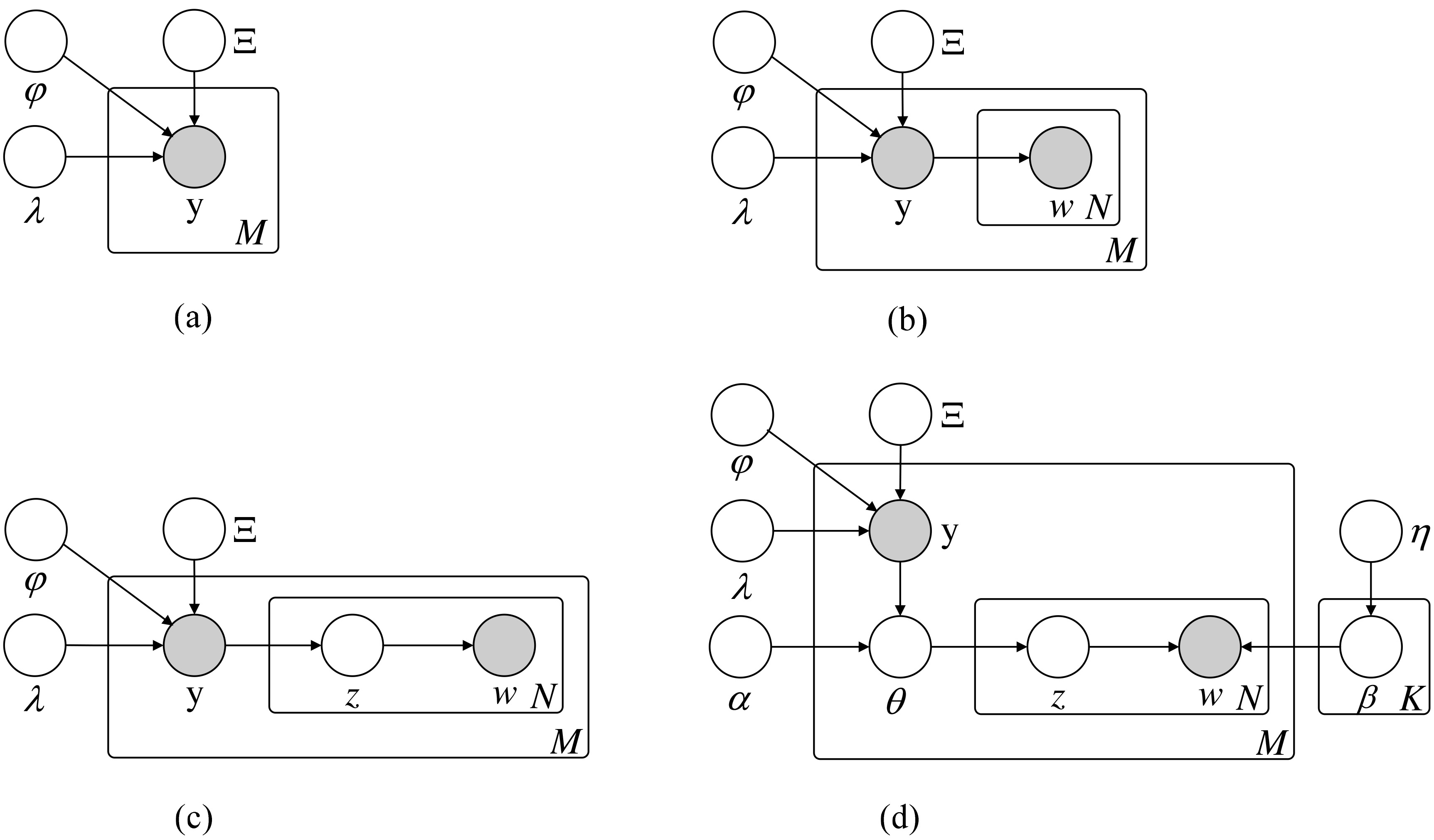
$\begin{split}\displaystyle P(\textbf{y},\textbf{d}|\lambda,\varphi,\Xi)=P(% \textbf{d}|\textbf{y})P(\textbf{y}|\lambda,\varphi,\Xi).\end{split}$ (2)

Figure 1.
Graphical model representation for label correlation mixture model, in which the labels and words are both observed variables. (a): LCM (label correlation model). (b): LCM+MoLM. The MoLM here is the mixture of unigram language model. (c): LCM+PLSA [10, 11]. The PLSA here can be viewed as a special supervised version. (d) LCM+LDA. The LDA here can be considered as a supervised form similar to L-LDA [16].

In Eq. (2), $P(\textbf{y}|\lambda,\varphi,\Xi)$ corresponds to the label correlation model, which depicts labels’ stochastic generative process, denoted as S1. Figure 1a shows the probabilistic graphical model. Because there exist $L!$ different orders (or sequences) of labels to generate a subset y, all of these orders should be summed over to calculate the probability:

$P(\textbf{y}|\lambda,\varphi,\Xi)=P(L|\lambda)\cdot\sum_{S_{L}\in\Phi_{\textbf% {y}}}P(S_{L}|\varphi,\Xi)$ (3)

where $\Phi_{\textbf{y}}$ denotes all the possible orders of labels in y,

$\displaystyle\Phi_{\textbf{y}}=\{(y_{\pi(1)},y_{\pi(2)},\ldots y_{\pi(L)})\mid% (\pi(1),\pi(2),\ldots,\pi(L))\in\ \ \{\text{all the permutations of the % integers from 1 to $L$}\}\}.$

Suppose $S_{L}=(y_{\pi(1)},y_{\pi(2)},...,y_{\pi(L)})$ ; then, we have

$\displaystyle P(S_{L}|\varphi,\Xi)=P(y_{\pi(1)}|\varphi)\cdot P(y_{\pi(2)}|\{y% _{\pi(1)}\},\Xi)\cdot\ldots\cdot P(y_{\pi(L)}|\{y_{\pi(1)},y_{\pi(2)},...,y_{% \pi(L-1)}\},\Xi).$ (4)

Equation (4) is the key point for calculating Eq. (3). We describe our approach to Eqs (3) and (4) in Section 4.

In Eq. (2), $P(\textbf{d}|\textbf{y})$ represents the label mixture model, which formulates the words’ generative process, denoted as S2, when the label subset y is given. S2 is a general description for words’ generative process. Regarding its concrete form, several different models can be chosen. The mixture of language models (MoLM), PLSA and LDA are three common generative models for text. From Fig. 1b to d, we present the graphical models of these three kinds of models, which are integrated with the label correlation model displayed in Fig. 1a. Section 5 discusses the details of the label mixture model employed in this paper.

Figure 2.
Two examples of the calculation of $P(y^{\prime}|\textbf{y},\Xi)$ based on a label correlation network with nine vertexes (labels). In subgraph (a), the conditional probability of selecting label $2$ when label $5$ is given, i.e. $P(2|\{5\},\Xi)$ , can be calculated by $P(2|\{5\},\Xi)=\frac{\kappa(\{5\},2)}{\sum_{y^{\prime\prime}\in\{2,3,4,6,8,9\}% }\kappa(\{5\},y^{\prime\prime})}=\frac{\xi(5,2)}{\sum_{y^{\prime\prime}\in\{2,% 3,4,6,8,9\}}\xi(5,y^{\prime\prime})}.$ Regarding subgraph (b), $P(3|\{2,5,8\},\Xi)$ is the conditional probability of selecting label $3$ based on label subset $\{2,5,8\}$ , and can be calculated by $P(3|\{2,5,8\},\Xi)=\frac{\kappa(\{2,5,8\},3)}{\sum_{y^{\prime\prime}\in\{1,3,4% ,6,9\}}\kappa(\{2,5,8\},y^{\prime\prime})}=\frac{\xi(2,3)+\xi(5,3)}{\sum_{y^{% \prime\prime}\in\{1,3\}}\xi(2,y^{\prime\prime})+\sum_{y^{\prime\prime}\in\{3,4% ,6,9\}}\xi(5,y^{\prime\prime})+\sum_{y^{\prime\prime}\in\{6\}}\xi(8,y^{\prime% \prime})}.$ Only the relevant weights are displayed in the two subgraphs.

4. Label correlation model

The estimation of the prior probability $P(\textbf{y}|\lambda,\varphi,\Xi)$ in Eqs (2) and (3) is important, but presents difficulties for multi-label classification. On the one hand, formulating the relationship between labels, crucial for classification performance, creates challenges. On the other hand, since the number of multi-label classes (i.e. label subsets) is $2^{K}-1$ , the relative sparsity of data distribution makes estimating parameters difficult for all these subsets, even when $K$ is not very large. In this section, we propose our approach to formulating the generative process of labels, accounting for the dependency between labels. We present an efficient algorithm to calculate $P(\textbf{y}|\lambda,\varphi,\Xi)$ , and then discuss the parameter-learning procedure for the model.

4.1 Label correlation network

We define a label correlation network employing an undirected graph, in which each vertex represents a single label, each edge between two vertexes indicates the correlation of the two corresponding labels, and the weight on each edge represents a certain measure for the correlation. Our basic assumption is that labels are generated based on the label correlation network, and $P(y_{l}|\textbf{y},\Xi)$ in the generative process S1-(c) can be calculated via the label correlation network. Here, we assume that the label correlation network has been set up. In Section 4.3, we discuss how to create a label correlation network and how to learn its parameters.

Denote $g(y,y^{\prime})$ as the edge between the two vertexes which corresponds to label $y$ and label $y^{\prime}$ , and denote $\xi(y,y^{\prime})$ as the weight on $g(y,y^{\prime})$ . Define $\Xi$ as all the weights in the label correlation network:

$\Xi=\{\xi(y,y^{\prime})|y\neq y^{\prime},y\in\textbf{Y},y^{\prime}\in\textbf{Y% }\}.$

$\overline{\textbf{y}}$ denotes the complementary set of a label subset y,

$\overline{\textbf{y}}=\textbf{Y}\setminus\textbf{y}.$

$\textbf{y}^{*}$ denotes the candidate set of y,

$\textbf{y}^{*}=\{y^{\prime}|\exists g(y,y^{\prime}),y\in\textbf{y},y^{\prime}% \in\overline{\textbf{y}}\}.$

Given a subset y, suppose that another label $y^{\prime}$ will be sampled. Our basic idea is that the label $y^{\prime}$ should be chosen from the “candidate set” $\textbf{y}^{*}$ , because $\textbf{y}^{*}$ includes all the labels that connect to at least one label in y. Denote $P(y^{\prime}|\textbf{y},\Xi)$ as the conditional probability of choosing a label $y^{\prime}$ when a subset y is given. This is another form of $P(y_{l}|\textbf{y},\Xi)$ in the generative process S1-(c), and we suppose it can be calculated by:

$\displaystyle P(y^{\prime}|\textbf{y},\Xi)=\frac{\kappa(\textbf{y},y^{\prime})% }{\sum_{y^{\prime\prime}\in\textbf{y}^{*}}\kappa(\textbf{y},y^{\prime\prime})}% =\frac{\sum_{y\in\textbf{y}}\xi(y,y^{\prime})}{\sum_{y^{\prime\prime}\in% \textbf{y}^{*}}\sum_{y\in\textbf{y}}\xi(y,y^{\prime\prime})},y^{\prime}\in% \textbf{y}^{*}$ (5)

where $\kappa(\textbf{y},y^{\prime})=\sum_{y\in\textbf{y}}\xi(y,y^{\prime})$ . According to Eq. (5), $\sum_{y^{\prime}\in\textbf{y}^{*}}P(y^{\prime}|\textbf{y},\Xi)=1$ , which means that $y^{\prime}$ is randomly generated under a multinomial distribution with parameters determined by Eq. (5). Figure 2 shows two examples of how to calculate the conditional probability of sampling a new label according to Eq. (5) based on the label correlation network.

Figure 3.

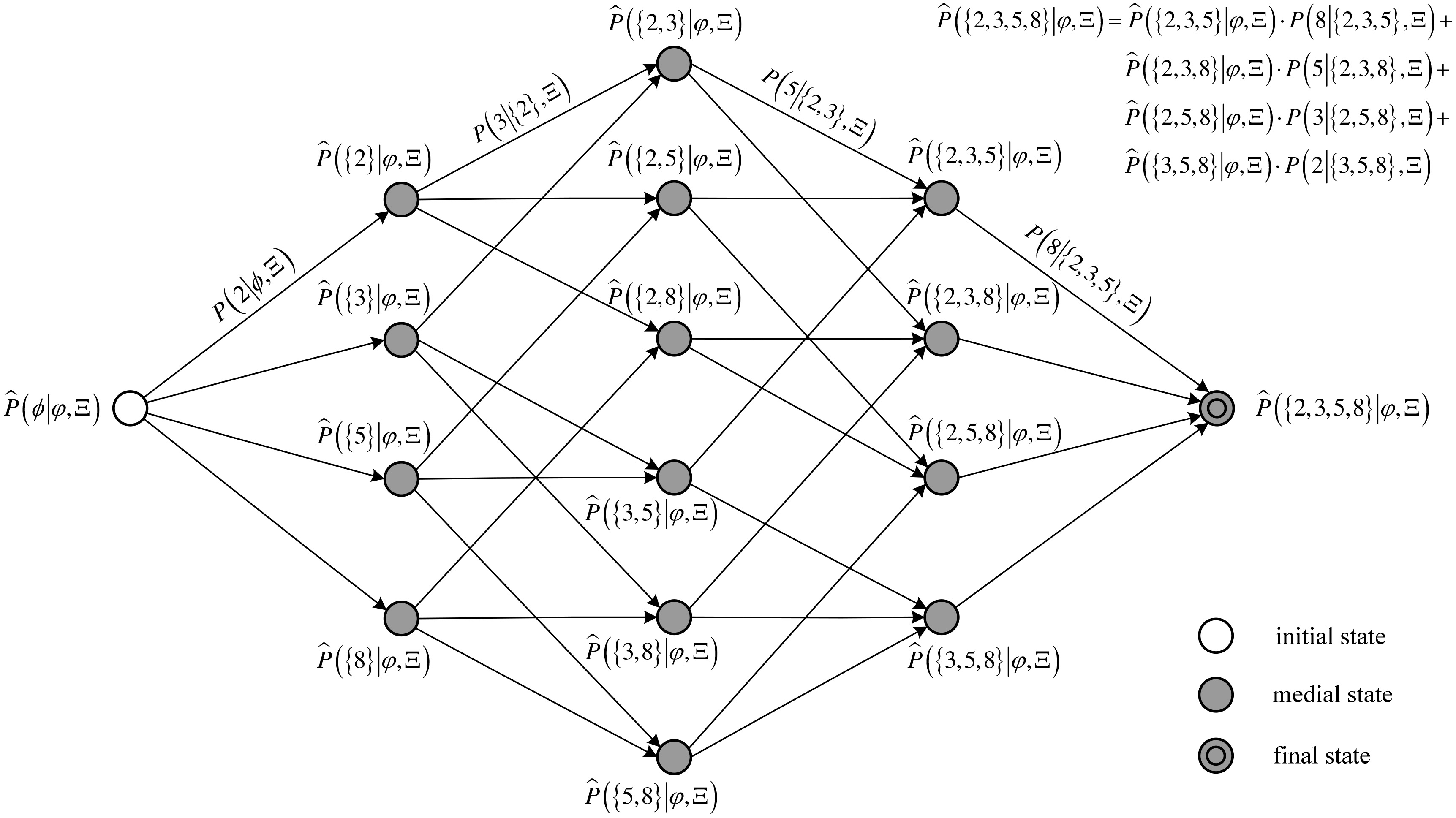
An example of FSM for calculating state score $\widehat{P}(\textbf{y}|\varphi,\Xi)$ , in which y contains four labels with the label indexes $2$ , $3$ , $5$ , $8$ . The FSM can be displayed via a directed acyclic graph with a trellis structure. Four transition probabilities, $P(2|\phi,\Xi)$ , $P(3|\{2\},\Xi)$ , $P(5|\{2,3\},\Xi)$ , $P(8|\{2,3,5\},\Xi)$ , are displayed; other transition probabilities are ignored.

4.2 Inference based on label correlation network

We denote $\widehat{P}(\textbf{y}|\varphi,\Xi)$ as the second term of the RHS of Eq. (3):

$\displaystyle\widehat{P}(\textbf{y}|\varphi,\Xi)=\sum_{S_{L}\in\Phi_{\textbf{y% }}}P(S_{L}|\varphi,\Xi)$ (6)

This is the key point in Eq. s(3). sIn theory, $\widehat{P}(\textbf{y}|\varphi,\Xi)$ should be computed by summing over all the $L!$ possible label orders’ probabilities, in which each order has $L-1$ times of multiplication operation. According to the Stirling’s approximation:

$L!\approx\sqrt{2\pi L}\cdot(L/e)^{L}$

the total computational requirements are on the order of $L^{3/2}\cdot(L/e)^{L}$ operations. This complexity greatly influences the computational efficiency, which is unaffordable. As a result, we propose an equivalent algorithm for calculating $\widehat{P}(\textbf{y}|\varphi,\Xi)$ , which can easily alleviate the exorbitant computational requirements.

We appeal to finite state machine (FSM) to illustrate the algorithm. In an FSM associated with y, a state is defined to represent a subset of y. Each subset maintains a one-to-one correspondence to a state. There are three kinds of states:

Initial state: corresponds to the empty subset, $\phi$ ;

Medial state: corresponds to the proper subset of y, except for the empty subset;

Final state: corresponds to y itself.

Suppose u is a subset of y, denote st(u) as the state which corresponds to u. Furthermore, we denote $\textbf{u}^{\textit{pre}}$ as the precursor set of u, and denote st( $\textbf{u}^{\textit{pre}}$ ) as the precursor state of st(u). $\textbf{u}^{\textit{pre}}$ meets the following condition:

$|\textbf{u}^{\textit{pre}}|+1=|\textbf{u}|,\ \textbf{u}^{\textit{pre}}\subset% \textbf{u}$

where $|\cdot|$ represents the subset’s size, and there are $|\textbf{u}|$ precursor sets of u. A transition in the FSM refers to the probability of transiting from one state to another. A transition to st(u) can only comes from one of its precursor states. In addition, the transition probability is defined as the conditional probability of generating u when $\textbf{u}^{\textit{pre}}$ is given, i.e. $P(\textbf{u}-\textbf{u}^{\textit{pre}}|\textbf{u}^{\textit{pre}},\Xi)$ , which can be calculated by Eq. (5). We also define the state score of st(u) as $\widehat{P}(\textbf{u}|\varphi,\Xi)$ , which is displayed in Eq. (6).

According to the above description, the FSM utilized in this paper can be represented by a directed acyclic graph. Figure 3 displays an example of an FSM associated with four labels. In the FSM, a complete path from the initial state st( $\phi$ ) to the final state st(y) corresponds to an order of all the labels in y. We define the path score as the product of all the transition probabilities, which is equal to the probability of generating the corresponding order of labels, i.e. $P(S_{L}|\varphi,\Xi)$ in Eq. (4). $\widehat{P}(\textbf{y}|\varphi,\Xi)$ , the state score of st(y), can be calculated by summing over all of the path scores in the FSM without complexity constraints.

Reducing the complexity of calculating $\widehat{P}(\textbf{y}|\varphi,\Xi)$ to an acceptable order presents a challenge. Fortunately, the paradigm of forward algorithm[19, 20] can be applied. The forward algorithm is widely utilized for hidden Markov model. We call our algorithm the forward sampling algorithm, due to its similar properties to the forward algorithm. Figure 3 shows that the state score of st(u) can be calculated by:

$\displaystyle\widehat{P}(\textbf{u}|\varphi,\Xi)=\sum_{\textbf{u}^{\textit{pre% }}}\widehat{P}(\textbf{u}^{\textit{pre}}|\varphi,\Xi)\cdot P(\textbf{u}-% \textbf{u}^{\textit{pre}}|\textbf{u}^{\textit{pre}},\Xi).$ (7)

This indicates that u’s state score involves two parts. The first one is the state score of st( $\textbf{u}^{\textit{pre}}$ ), and the second one is the transition probability from st( $\textbf{u}^{\textit{pre}}$ ) to st(u). This also holds true for y,

$\displaystyle\widehat{P}(\textbf{y}|\varphi,\Xi)=\sum_{\textbf{y}^{\textit{pre% }}}\widehat{P}(\textbf{y}^{\textit{pre}}|\varphi,\Xi)\cdot P(\textbf{y}-% \textbf{y}^{\textit{pre}}|\textbf{y}^{\textit{pre}},\Xi).$ (8)

From the perspective of the label rather than that of subset, Eq. (8) also has an equivalent formula:

$\displaystyle\widehat{P}(\textbf{y}|\varphi,\Xi)=\sum_{y\in\textbf{y}}\widehat% {P}(\textbf{y}\setminus\{y\}|\varphi,\Xi)\cdot P(y|\textbf{y}\setminus\{y\},% \Xi).$ (9)

The calculation of the state score does not require computing all of the path scores. Instead, this calculation only involves the state scores of its precursor sets and the transition probabilities. This divide-and-conquer strategy significantly alleviates computational complexity. The operation requirement can be reduced to $L^{3/2}\cdot 2^{L}$ , which is an upper bound order. Although this is an exponential order, it is acceptable in most cases. On the one hand, the actual number of labels for a document may not be very large. On the other hand, the size of y, i.e. $L$ , can be limited in a reasonable range, which is relevant to the classification strategy discussed in Section 6 that can further improve the efficiency of the multi-label classification.

4.3 Parameter learning of

\Xi

in the label correlation network

For parameter learning, we first set up and initialized the label correlation network based on the observed multi-label classes in the training data set. Since the frequency of co-occurrence is a typical representation for the correlation between two labels, in the current paper, we directly employ the raw counts of co-occurrence for the weights’ initialization. If two labels co-occur in the training set, the weight on the corresponding edge is set to the co-occurrence count. In addition, if two labels do not co-occur in the training set, an edge exists between the two corresponding vertexes in the label correlation network, and we set the initial weight is set to one.

To obtain a more reasonable estimation for the prior probability $P(\textbf{y}|\lambda,\varphi,\Xi)$ in Eq. (2), all the weights in the label correlation network can be further optimized via utilizing certain criteria. In this paper, we choose the likelihood of all of the training data as the objective function, which maintains the following form:

$\displaystyle{{\cal L}}(\Xi)=\sum_{m=1}^{M}P(\textbf{y}_{m}|\lambda,\varphi,% \Xi).$ (10)

${{\cal L}}(\Xi)$ involves three kinds of parameters, $\lambda$ , $\varphi$ and $\Xi$ . Here, we only consider the weight parameter $\Xi$ , while we regard $\lambda$ and $\varphi$ as constant parameters whose estimation approaches are discussed in Section 4.4. The weights could be optimized by maximizing the objective function ${{\cal L}}(\Xi)$ . However, since the objective function is highly nonlinear for each weight, identifying the close form solution is difficult. The generalized probability descent (GPD) algorithm [21] is employed to seek the optimal $\Xi^{*}$ . Denote $\nabla{{\cal L}}(\Xi)$ as the gradient of ${{\cal L}}(\Xi)$ . The iterative GPD can be implemented as follows:

$\displaystyle\Xi_{t+1}=\Xi_{t}+\varepsilon_{t}\cdot\nabla{{\cal L}}(\Xi)|_{\Xi% _{t}}$ (11)

where $t$ is the iteration number, $\Xi_{t}$ represents the parameters at $t^{th}$ iteration; $\varepsilon_{t}$ is the learning rate; $\varepsilon_{t}=\varepsilon_{0}(1+t/T)$ ; $\varepsilon_{0}$ is the initial learning rate; and $T$ is the predefined maximum number of iterations.

We assign $\Xi$ another equivalent definition for the sake of simplicity:

$\Xi=\{\xi(p,q)|p\neq q,1\leqslant p\leqslant K,1\leqslant q\leqslant K\}$

where $\xi(p,q)$ represents the weight on the edge between the two vertexes, which correspond to label $y_{p}$ and label $y_{q}$ , respectively. Suppose the weight $\xi(p,q)$ will be optimized. The gradient of $\xi(p,q)$ can be written as:

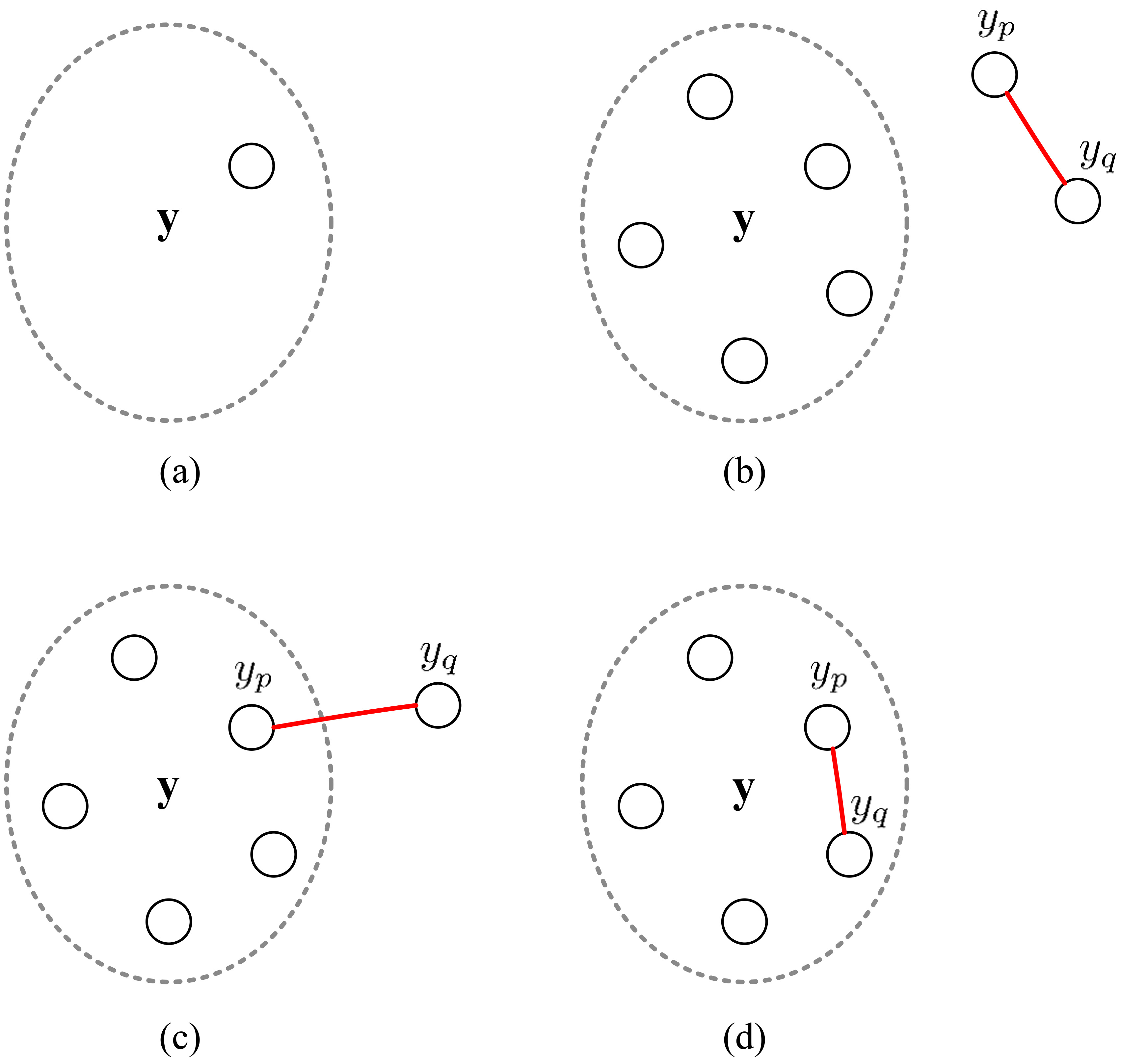
$\displaystyle\frac{\partial{{\cal L}}(\Xi)}{\partial\xi(p,q)}=\sum_{m=1}^{M}% \frac{\partial P(\textbf{y}_{m}|\lambda,\varphi,\Xi)}{\partial\xi(p,q)}=\sum_{% m=1}^{M}P(L|\lambda)\cdot\frac{\partial\widehat{P}(\textbf{y}_{m}|\varphi,\Xi)% }{\partial\xi(p,q)}.$ (12)

We focus on how to calculate the partial derivative of the state score $\widehat{P}(\textbf{y}_{m}|\varphi,\Xi)$ . Figure 4 displays four cases relevant to this calculation. The details of each case are described as (the subscript $m$ is ignored for brevity hereafter):

If $|\textbf{y}|<2$ , then:

$\displaystyle\frac{\partial\widehat{P}(\textbf{y}|\varphi,\Xi)}{\partial\xi(p,% q)}=0$

If $y_{p}\notin\textbf{y}$ , $y_{q}\notin\textbf{y}$ , then:

$\displaystyle\frac{\partial\widehat{P}(\textbf{y}|\varphi,\Xi)}{\partial\xi(p,% q)}=0$

If $y_{p}\in\textbf{y}$ , $y_{q}\notin\textbf{y}$ , then according to Eq. (9):

$\displaystyle\frac{\partial\widehat{P}(\textbf{y}|\varphi,\Xi)}{\partial\xi(p,% q)}=\sum_{y\in\textbf{y}}\left[\frac{\partial\widehat{P}(\textbf{y}\setminus\{% y\}|\varphi,\Xi)}{\partial\xi(p,q)}\cdot P(y|\textbf{y}\setminus\{y\},\Xi)% \right.\left.+\ \widehat{P}(\textbf{y}\setminus\{y\}|\varphi,\Xi)\cdot\frac{% \partial P(y|\textbf{y}\setminus\{y\},\Xi)}{\partial\xi(p,q)}\right].$ (13)

Regarding $\frac{\partial P(y|\textbf{y}\setminus\{y\},\Xi)}{\partial\xi(p,q)}$ , we can derive it according to Eq. (5) as:

If $y=y_{p}$ , then

$\displaystyle\frac{\partial P(y|\textbf{y}\setminus\{y\},\Xi)}{\partial\xi(p,q% )}=0$

If $y\neq y_{p}$ , then

$\displaystyle\frac{\partial P(y|\textbf{y}\setminus\{y\},\Xi)}{\partial\xi(p,q% )}=\frac{-\kappa(\textbf{y}\setminus\{y\},y)}{{\left[\sum_{y^{\prime}\in(% \textbf{y}\setminus\{y\})^{*}}\kappa(\textbf{y}\setminus\{y\},y^{\prime})% \right]}^{2}}$

where $(\textbf{y}\setminus\{y\})^{*}$ is the candidate set of $\textbf{y}\setminus\{y\}$ . In addition, if $y_{p}\notin\textbf{y}$ and $y_{q}\in\textbf{y}$ , we have the same inference process except for exchanging $y_{p}$ and $y_{q}$ , which is not presented here.

If $y_{p}\in\textbf{y}$ , $y_{q}\in\textbf{y}$ , then we can also obtain Eq. (13). As for $\frac{\partial P(y|\textbf{y}\setminus\{y\},\Xi)}{\partial\xi(p,q)}$ :

If $y\neq y_{p}$ and $y\neq y_{q}$ , then

$\displaystyle\frac{\partial P(y|\textbf{y}\setminus\{y\},\Xi)}{\partial\xi(p,q% )}=0$

If $y=y_{p}$ , then

$\displaystyle\frac{\partial P(y|\textbf{y}\setminus\{y\},\Xi)}{\partial\xi(p,q% )}=\frac{\left[\sum_{y^{\prime}\in(\textbf{y}\setminus\{y\})^{*}}\kappa(% \textbf{y}\setminus\{y\},y^{\prime})\right]-\kappa(\textbf{y}\setminus\{y\},y)% }{{\left[\sum_{y^{\prime}\in(\textbf{y}\setminus\{y\})^{*}}\kappa(\textbf{y}% \setminus\{y\},y^{\prime})\right]}^{2}}$

If $y=y_{q}$ , the inference process is the same as the above.

Figure 4.

Different cases for the partial derivative of y’s state score.

In Eq. (13), $P(y|\textbf{y}\setminus\{y\},\Xi)$ and $\widehat{P}(\textbf{y}\setminus\{y\}|\varphi,\Xi)$ can be calculated utilizing Eqs (5) and (9), respectively. $\frac{\partial\widehat{P}(\textbf{y}\setminus\{y\}|\varphi,\Xi)}{\partial\xi(p% ,q)}$ can be deduced by Eq. (13) itself recursively. Therefore, from Eq. (13) we can observe that the paradigm of the forward algorithm can be reapplied to obtain the partial derivative. This resembles the inference process described in Section 4.2. We call this learning algorithm the forward gradient algorithm.

4.4 Parameter estimation of

\lambda

and

\varphi

$\lambda$ and $\varphi$ are two vector parameters of multinomial distribution employed in the generative process S1. $\lambda$ is a $K$ dimensional vector $(\lambda_{1},\lambda_{2},\ldots,\lambda_{K})$ , in which $\lambda_{k}(1\leqslant k\leqslant K)$ represents the probability of containing $k$ labels for a subset, and $\sum_{k=1}^{K}\lambda_{k}=1$ . $\lambda_{k}$ can be easily estimated by $c^{\lambda}_{k}/\sum_{k=1}^{K}c^{\lambda}_{k}$ , where $c^{\lambda}_{k}$ is the count of subsets that contain $k$ labels in the training data set. $\varphi$ is also a $K$ dimensional vector $(\varphi_{1},\varphi_{2},\ldots,\varphi_{K})$ , where $\varphi_{k}(1\leqslant k\leqslant K)$ is the probability of attaining the $k^{th}$ label in the generative process for the first label in S1-(b), and $\sum_{k=1}^{K}\varphi_{k}=1$ . $\varphi_{k}$ in the current paper is estimated by $c^{\varphi}_{k}/\sum_{k=1}^{K}c^{\varphi}_{k}$ , where $c^{\varphi}_{k}$ is the count of the $k^{th}$ single label in the training data set. In our experiments, $\lambda$ and $\varphi$ are both smoothed via the laplace smoothing method [22].

5. Label mixture model

5.1 Different choices

As described in Section 3, the label mixture model corresponds to S2, which formulates the generative process of words in a document with given labels. Many traditional generative mixture models can be chosen and embedded into S2, such as the mixture of language models, PLSA, LDA, etc. Different models maintain different generative process assumptions. In the current paper, we adopt LDA as the label mixture model. Figure 1d displays the overall graphical model. Since labels are visible in the training data, parameters of these models should be learned in a supervised manner, in which the labels of a document are restricted to belonging to a known label subset. This varies from the traditional models. The parameter learning procedure can be the same as that of the L-LDA. After parameter training, only $\{\beta_{k}|1\leqslant k\leqslant K\}$ , the parameters of labels’ multinomial distribution over words, are utilized in multi-label classification stage.

5.2 Fold-in process

Given a new document $\textbf{d}^{\prime}$ , a label subset y for $\textbf{d}^{\prime}$ , and the model displayed in Fig. 1d, the fold-in process can be applied to obtain the optimal joint probability of $\textbf{d}^{\prime}$ and the vector variable $\theta$ , which is a multinomial mixture distribution over labels. This optimization problem can be written as:

$\displaystyle\theta^{*}=\operatorname*{argmax}_{\theta}P(\textbf{d}^{\prime},% \theta|\textbf{y},\alpha,\beta)\operatorname*{argmax}_{\theta}P(\textbf{d}^{% \prime}|\theta,\textbf{y},\beta)P(\theta|\textbf{y},\alpha).$ (14)

This fold-in process resembles that of PLSA [13, 10, 23], except for two differences. The first difference is that, in Eq. (14) the labels involved in $\theta$ are limited within y, whereas in PLSA, all of the labels are taken into account. The second difference is that the term $P(\theta|\textbf{y},\alpha)$ should be calculated, while in PLSA only the term $P(\textbf{d}^{\prime}|\theta,\textbf{y},\beta)$ is considered. Regarding the optimization method, Gibbs sampling [24] or EM algorithm can be chosen to obtain the optimal $\theta^{*}$ .

6. Multi-label classification strategy

As described in Section 1, the goal of multi-label text classification is to find the optimal subset $\hat{\textbf{y}}$ in Y for a new document $\textbf{d}^{\prime}$ . According to Bayes decision theory, all possible subsets should be assessed in theory. However, the number of multi-label classes is an exponential function ( $2^{K}-1$ ) of the label set size, $K$ . We propose a two-step strategy to solve this problem:

Coarse Selection (CS): Obtain a label subset $\textbf{Y}^{CS}$ ( $\textbf{Y}^{CS}\subseteq\textbf{Y}$ ), in which the labels maintain relatively higher probabilities associated with $\textbf{d}^{\prime}$ . Recall performance and efficiency are two basic goals for this step. In theory, any reasonable approach can be adopted to achieve this goal. In the current paper, we employ two binary relevance methods [1] based on simple classifiers. Section 7.2 describes the details of our implementation.

Refined Assessment: Assessing all of the multi-label classes in $\textbf{Y}^{CS}$ for document $\textbf{d}^{\prime}$ utilizing the LCMM (based on the model displayed in Fig. 1d):

$\displaystyle\hat{\textbf{y}}=\operatorname*{argmax}_{\textbf{y}\subseteq% \textbf{Y}}P(\textbf{y}|\textbf{d}^{\prime},\lambda,\phi,\Xi,\alpha,\beta)=% \operatorname*{argmax}_{\textbf{y}\subseteq\textbf{Y}}\frac{P(\textbf{d}^{% \prime}|\textbf{y},\alpha,\beta)P(\textbf{y}|\lambda,\phi,\Xi)}{P(\textbf{d}^{% \prime}|\lambda,\phi,\Xi,\alpha,\beta)}=\operatorname*{argmax}_{\textbf{y}% \subseteq\textbf{Y}}P(\textbf{d}^{\prime}|\textbf{y},\alpha,\beta)P(\textbf{y}% |\lambda,\phi,\Xi)\approx\operatorname*{argmax}_{\textbf{y}\subseteq\textbf{Y}% ^{CS}\subseteq\textbf{Y}}P(\textbf{d}^{\prime}|\textbf{y},\alpha,\beta)P(% \textbf{y}|\lambda,\phi,\Xi).$ (15)

$P(\textbf{y}|\lambda,\phi,\Xi)$ can be calculated employing the label correlation model described in Section 4. $P(\textbf{d}^{\prime}|\textbf{y},\alpha,\beta)$ can be calculated as follows:

$\displaystyle P(\textbf{d}^{\prime}|\textbf{y},\alpha,\beta)=\int\left(\prod_{% n=1}^{N}\sum_{z_{n}\in\textbf{y}}P(z_{n}|\theta,\textbf{y})P(w_{n}|z_{n},% \textbf{y})\right)P(\theta|\textbf{y},\alpha)d\theta$

where $N$ is the number of words in $\textbf{d}^{\prime}$ ; $w_{n}$ is the $n^{th}$ word in $\textbf{d}^{\prime}$ ; $z_{n}$ is the $n^{th}$ label assignment for $w_{n}$ . This is an intractable function because of the coupling between $\theta$ and $P(w_{n}|z_{n},\textbf{y})$ in the summation. Since the goal of multi-label classification is to identify the best label subset, the integral could be approximated with the maximum to find the best joint probability of $\textbf{d}^{\prime}$ and $\theta$ utilizing the fold-in process, Eq. (14). Therefore, the Eq. (15) can be modified as follows:

$\displaystyle\hat{\textbf{y}}\approx\operatorname*{argmax}_{\textbf{y}% \subseteq\textbf{Y}^{CS}\subseteq\textbf{Y}}P(\textbf{d}^{\prime}|\textbf{y},% \alpha,\beta)P(\textbf{y}|\lambda,\phi,\Xi)\approx\operatorname*{argmax}_{% \textbf{y}\subseteq\textbf{Y}^{CS}\subseteq\textbf{Y}}\left\{\left[\max_{% \theta}P(\textbf{d}^{\prime},\theta|\textbf{y},\alpha,\beta)\right]P(\textbf{y% }|\lambda,\phi,\Xi)\right\}.$ (16)

Equation (16) represents our overall solution based on LCMM for the multi-label text classification.

7. Experiments

7.1 Data sets and evaluation measures

In our experiments, we utilize three original text classification data sets downloaded from the Internet to evaluate the performance of the LCMM: Reuters-21578 [25], TMC2007 [26] and OHSUMED.1 Reuters-21578 is a collection of articles that appeared in the 1987 Reuters newswire, a standard text classification benchmark. We utilize the Mod-Apte split, as descried in the “README” file accompanying the original set. This data set is named Reuters-all90 in this paper, and contains 90 labels. Two subsets of Reuters-all90 are also employed in these experiments. The subsets only utilize 10 and 36 labels [6, 15, 17], which are called Reuters-top10 and Reuters-top36, respectively. TMC2007 is a data set regarding aviation safety reports, comprising records of the problems that occurred during flights. OHSUMED includes medical abstracts from the MeSH categories of the year 1991. Table 2 presents the details of the data sets.

Various kinds of evaluation measures are employed: accuracy, precision, recall, F-score, micro/macro F-score. The details of these evaluation measures are described in [1, 27].

Table 2
Data sets collection and statistics. #trn refers to the number of training documents. #tst indicates the number of testing documents. #lbl is the number of labels. l-card indicates label cardinality [1], the average number of labels relevant to each document

Data set	#TRN	#TST	#LBL	L-CARD
Reuters-top10	6490	2544	10	1.10
Reuters-top36	7543	2906	36	1.19
Reuters-all90	7768	3019	90	1.24
TMC2007	21519	7077	22	2.16
OHSUMED	6965	6964	23	1.67

7.2 Experimental setup

Simple preprocessing is conducted on each data set. Meaningless tags and numbers are removed. All words are converted to lowercase, and the words on a standard stop word list of about 400 words are removed. Stemming is performed by Porters stemmer [28]. In addition, term selection [29, 30] is performed utilizing the $\chi^{2}$ (Chi-square) function with a reduction factor of $0.9$ .

The label correlation model is trained according to the learning approach described in Section 4.3. The label mixture model is trained directly utilizing the JGibbLabeledLDA package2 with the default parameter configuration. Regarding the two-step multi-label classification strategy, the binary relevance method (BM) [1] is employed in the coarse selection step. The approach learns a set of binary classifiers for each label $y_{k}$ $(1\leqslant k\leqslant K)$ and gives the $0/1$ prediction of each label for a document. Here $0$ means the label does not belong to the document, and $1$ has the opposite meaning. Various kinds of traditional models can be employed to build the binary classifiers. In our experiments, the naive Bayes (NB) model [1] and the SVM model [29, 31, 32] are implemented. For the naive Bayes model, the binary classifier can be formulated as:

$\log P(\textbf{d}|y^{1}_{k})P(y^{1}_{k})-\log P(\textbf{d}|y^{0}_{k})P(y^{0}_{% k})>\tau,\ 1\leqslant k\leqslant K$

where $\tau$ is a constant that controls the classification boundary. When $\tau=0$ (default), this is the traditional naive Bayes binary classifier. Regarding SVM, the classifiers is implemented via the $\text{SVM}^{\text{light}}$ toolkit3 [32]. For the features utilized in the SVM model, we adopt the term weighting policy:

$tf\text{-}\chi^{2}(w_{n},\textbf{d})=tf(w_{n},\textbf{d})\cdot\chi^{2}(w_{n})$

where $\chi^{2}(w_{n})$ is the chi-square of word $w_{n}$ , and

$\displaystyle tf(w_{n},\textbf{d})=\begin{cases}1+\log\#(w_{n},\textbf{d}),\ % \ \#(w_{n},\textbf{d})>0\\ 0,\ \ \text{otherwise}\end{cases}$

$\#(w_{n},\textbf{d})$ is the frequency of word $w_{n}$ in document d. This resembles the $tf\text{-}idf$ term weighting approach.

In the coarse selection step, we should try to guarantee that the actual label are included in $\textbf{Y}^{\text{CS}}$ , so the configuration of the approach is different from the default configuration. For the NB classifiers, $\tau$ is set to $-80.0$ to enhance the recall performance. For the SVM classifiers, the trade-off parameter (“-c” option) is set to $5.0$ , the cost-factor (“-j” option) is set to $1.5$ . All of the parameters are set empirically on the training data set.

Table 3
Performance comparison on Reuters. (“ $-$ ” indicates that the performance of the corresponding approach was not reported in the paper)

	Reuters-top10			Reuters-top36			Reuters-all90
Approach	Precision	Recall	F-score	Precision	Recall	F-score	Precision	Recall	F-score
Mix-Model	0.839	$-$	$-$	$-$	$-$	$-$	$-$	$-$	$-$
ML-KNN	$-$	$-$	$-$	0.795	0.797	0.791	$-$	$-$	$-$
Mul-Model	$-$	$-$	$-$	$-$	$-$	$-$	0.852	0.720	$-$
Boostexter	$-$	$-$	$-$	$-$	$-$	$-$	$-$	$-$	0.851
CoL-Model	$\,\ \text{0.901}^{*}$	$\,\ \text{0.923}^{*}$	$\,\ \text{0.898}^{*}$	$\,\ \text{0.872}^{*}$	$\,\ \text{0.875}^{*}$	$\,\ \text{0.876}^{*}$	$\,\ \text{0.867}^{*}$	$\,\ \text{0.873}^{*}$	$\,\ \text{0.866}^{*}$
$\text{BMNB}^{\text{CS}}+\text{LCMM}^{\text{GPD}}$	0.935	0.965	0.940	0.906	0.929	0.905	0.901	0.915	0.895
$\text{BMSVM}^{\text{CS}}+\text{LCMM}^{\text{GPD}}$	0.959	0.973	0.961	0.939	0.947	0.935	0.924	0.930	0.918

Table 4

Performance comparison on reuters

	Reuters-top10		Reuters-all90
	Micro	Macro	Micro	Macro
Approach	F-score	F-score	F-score	F-score
Roc-Method	0.839	0.681	0.765	0.550
KNN	0.852	0.855	0.793	0.529
MFoM-Bin	0.933	0.883	0.884	0.556
MFoM-MC	$\,\ \text{0.937}^{*}$	$\,\ \text{0.884}^{*}$	$\,\ \text{0.888}^{*}$	$\,\ \text{0.630}^{*}$
$\text{BMNB}^{\text{CS}}+\text{LCMM}^{\text{GPD}}$	0.919	0.846	0.850	0.717
$\text{BMSVM}^{\text{CS}}+\text{LCMM}^{\text{GPD}}$	0.953	0.919	0.890	0.787

7.3 Experimental results

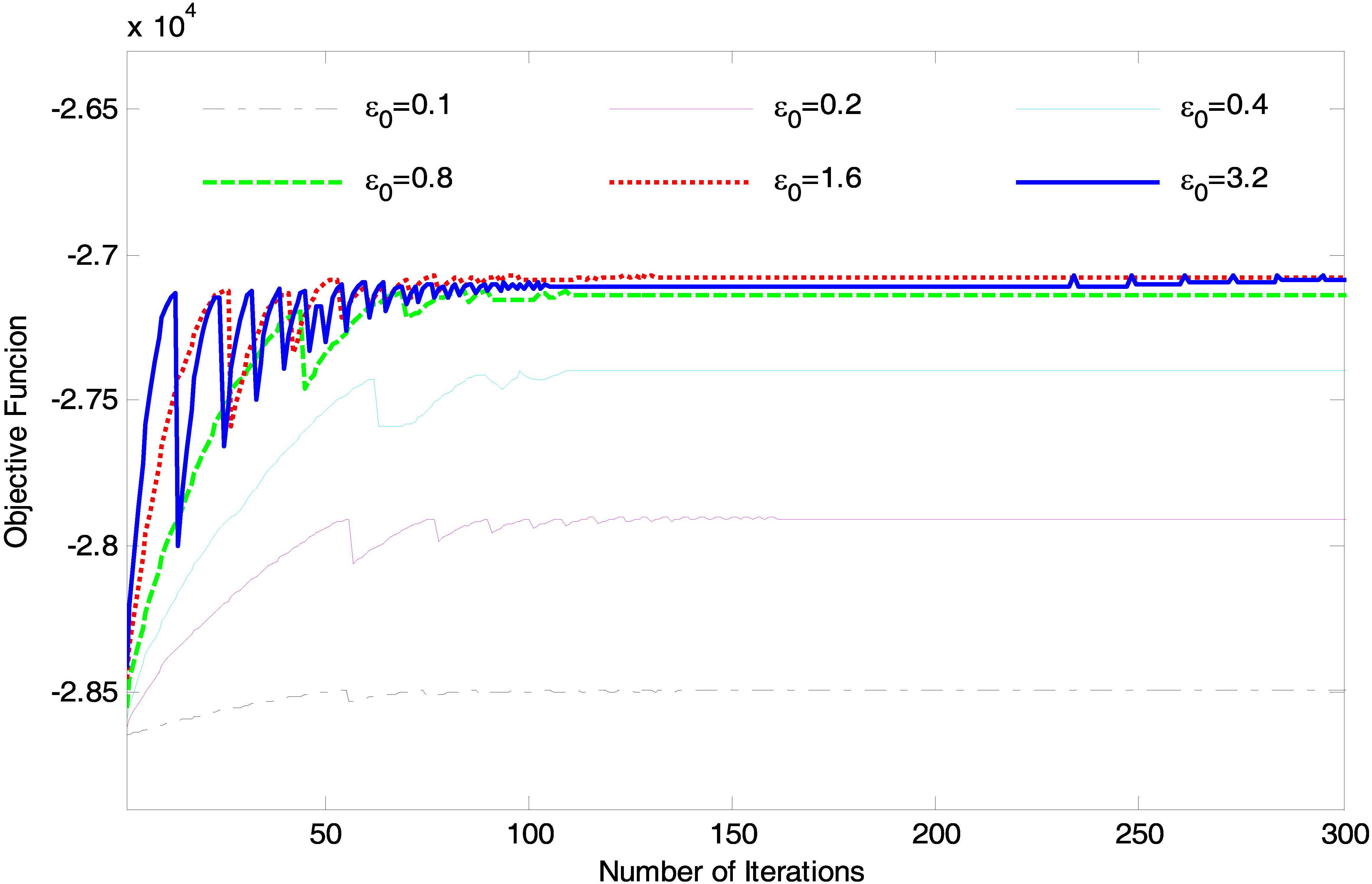
We first investigate the learning procedure for the weights of label correlation network, Fig. 5 shows different convergence curves of objective function values corresponding to different $\varepsilon_{0}$ on the TMC2007 data set. The maximum iteration number $T$ is set to $300$ . We can observe that objective functions for different $\varepsilon_{0}$ increase during the iterative training. All these curves reach stable stages after approximately $100$ iterations. These stable values increase with the $\varepsilon_{0}$ . However, when the $\varepsilon_{0}$ is larger than $0.8$ , the corresponding objective functions almost converge to the same value. We can also see that the larger the $\varepsilon_{0}$ is, the more fluctuant the convergence curve is, especially at the beginning of the iterative learning. Similar phenomena can be also observed from the convergence curves on the Reuters and OHSUMED data sets, which are not displayed in this paper. In our experiments, we obtain the optimal weights of the label correlation network on different data sets utilizing the same learning configuration: $\varepsilon_{0}=1.6$ and $120$ iterations.

Based on the optimized label correlation network, we implement two approaches denoted by $\text{BMNB}^{\text{CS}}+\text{LCMM}^{\text{GPD}}$ and $\text{BMSVM}^{\text{CS}}+\text{LCMM}^{\text{GPD}}$ , following the classification strategy described in Section 6. The $\text{BMNB}^{\text{CS}}$ represents the BM approach based on the NB model employing the coarse selection (CS) configuration, whereas $\text{BMSVM}^{\text{CS}}$ denotes the SVM-based coarse selection. In both approaches, the LCMM is adopted in the second refined assessment step, and we utilize the superscript “GPD” to denote the use of the optimized label correlation network. We compare the two approaches with other reported multi-label classification methods, including: Mixture Model (Mix-Model) [15]; CoL-Model [17]; ML-KNN [8, 17, 33]; Multinomial Model (Mul-Model) [34]; Boostexter [7, 17]; MFoM-Bin [5]; MFoM-MC [6]; Rocchio method (Roc-Method) [29]; KNN [29]; Ensemble-CC [3]; Ensemble-BM [3]; Ensemble-PS [3, 4]; RAKEL [3, 35].

Table 5
Performance comparison on TMC2007 and OHSUMED

	TMC2007		OHSUMED
		Macro		Macro
Approach	Accuracy	F-score	Accuracy	F-score
Ensemble-CC	$\,\ \text{0.530}^{*}$	0.551	0.411	0.378
Ensemble-BM	0.527	0.548	0.414	0.379
Ensemble-PS	0.523	$\,\ \text{0.561}^{*}$	$\,\ \text{0.420}^{*}$	0.376
RAKEL	0.529	0.557	0.416	$\,\ \text{0.398}^{*}$
$\text{BMNB}^{\text{CS}}+\text{LCMM}^{\text{GPD}}$	0.532	0.601	0.542	0.573
$\text{BMSVM}^{\text{CS}}+\text{LCMM}^{\text{GPD}}$	0.548	0.627	0.584	0.621

Figure 5.

Objective function convergence for different $\varepsilon_{0}$ with $300$ iterations.

Tables 3–5 presents the experimental results. Since different reported approaches were evaluated via different measures, and the data sets were also different, we list these reported experimental results and the corresponding ones of our approaches in the tables. The superscript “*” in the tables indicates the best reported results for a certain evaluation measure. We utilize the boldfaced value to denote the best result in its column.

From the three tables, we observe that $\text{BMNB}^{\text{CS}}+\text{LCMM}^{\text{GPD}}$ achieves good overall performance, $\text{BMSVM}^{\text{CS}}+\text{LCMM}^{\text{GPD}}$ outperforms all of the other methods. For Reuters data sets (Reuters-top10, Reuters-top36 and Reuters-all90), take the F-score measure as an example, The relative improvements are 61.8%, 47.6% and 38.8%, respectively. For the data sets TMC2007 and OHSUMED, performance is compared on the accuracy measure and the macro F-score measure; the relative improvements on TMC2007 are 3.8% and 15.0%, respectively; and for OHSUMED, the relative improvements achieve 28.3% and 37.0%, respectively.

Figure 6.

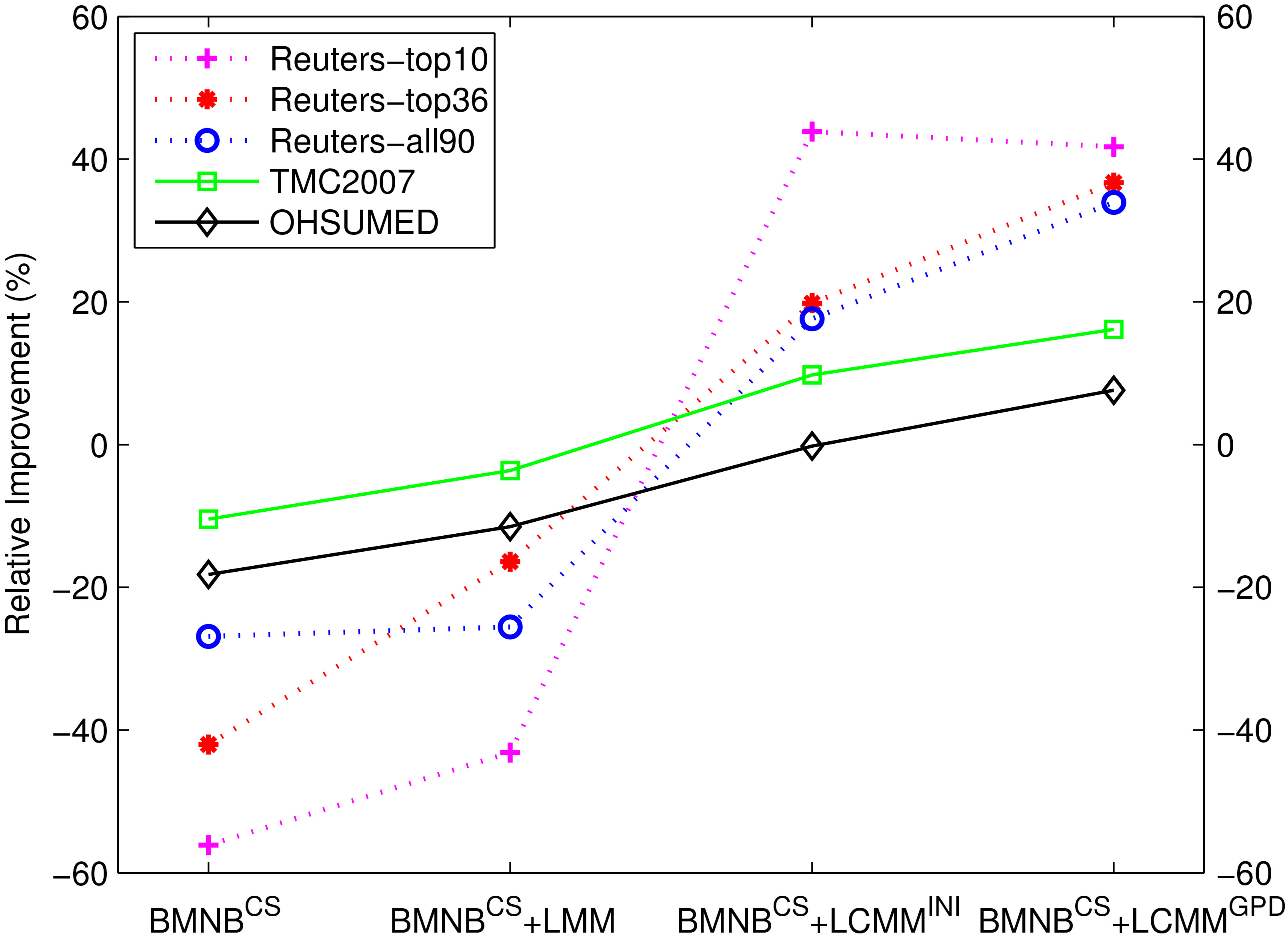
Relative micro F-score improvements of $\text{BMNB}^{\text{CS}}$ -based approaches compared with BMNB.

We further analyze our proposed approaches via more comparison. For $\text{BMNB}^{\text{CS}}+\text{LCMM}^{\text{GPD}}$ , we employ four methods:

BMNB: the BM approach based on NB model with the default NB configuration.

$\text{BMNB}^{\text{CS}}$ : only the $\text{BMNB}^{\text{CS}}$ based approach.

$\text{BMNB}^{\text{CS}}+\$ LMM: a two-step approach. In the second step only the label mixture model (LMM) is utilized, which means that the label correlation model, i.e. $P(\textbf{y}|\lambda,\phi,\Xi)$ , is ignored in the Eq. (16).

$\text{BMNB}^{\text{CS}}+\text{LCMM}^{\text{INI}}$ : a two-step approach. In the second step, the LCMM is adopted, but only the initial label correlation network is employed.

Similarly, we implement four approaches based on SVM methods to compare with $\text{BMSVM}^{\text{CS}}+\text{LCMM}^{\text{GPD}}$ . The comparison is conducted on micro/macro F-score evaluation measures, and Table 6 of Appendix A presents the complete experimental results.

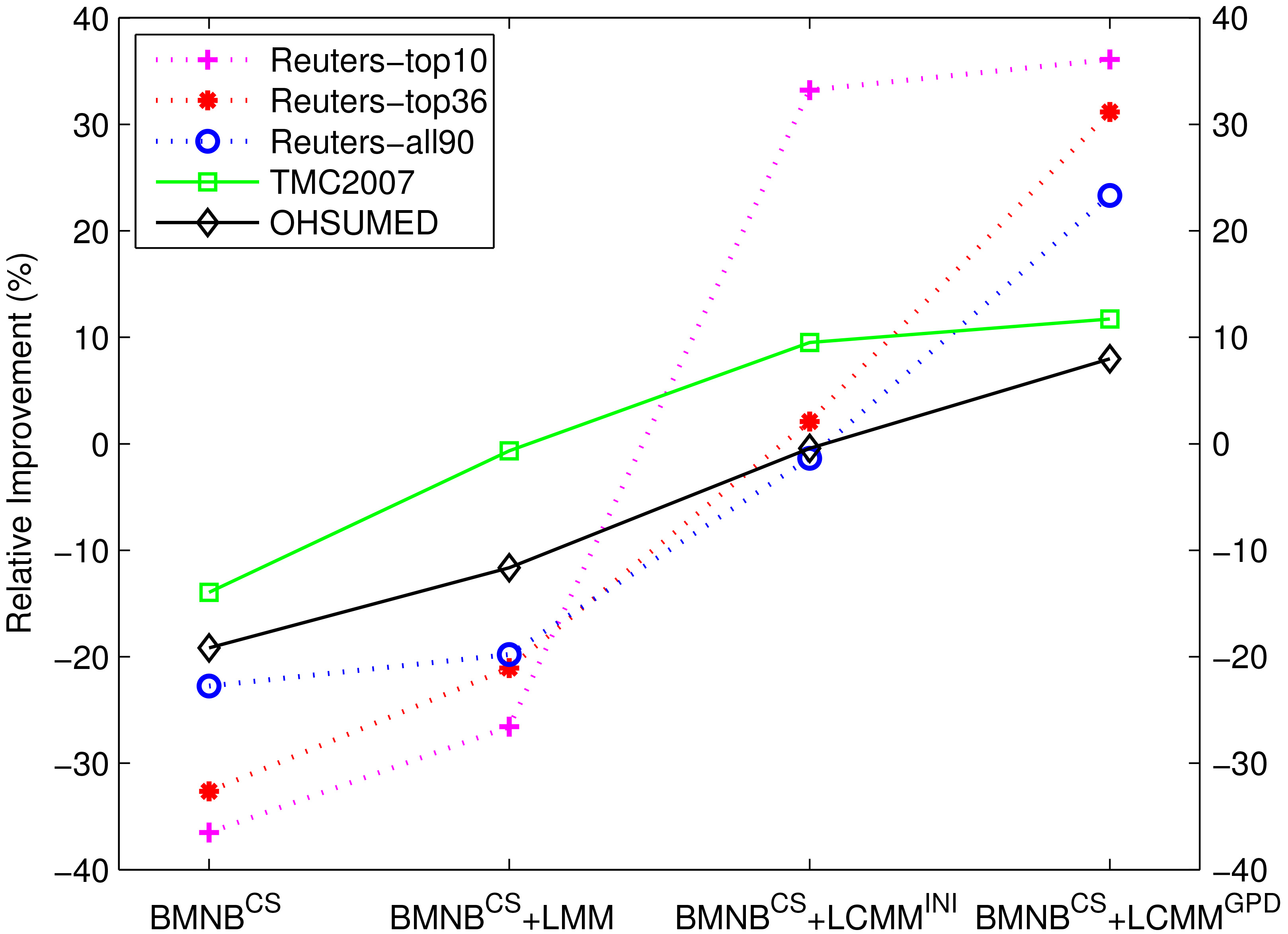
Since phenomena in NB-based methods and SVM-based methods are similar, this section only discusses NB-based methods, for illustration purposes. For the sake of clarity, we employ the performance of BMNB as the baseline, and compare all of the $\text{BMNB}^{\text{CS}}$ -based approaches with the BMNB. Figures 6 and 7 display the relative micro/macro F-score improvements. From the two figures, we can see that $\text{BMNB}^{\text{CS}}$ maintains the poorest performance in all of the data sets. Although it retains the best recall performance, its precision performance decreases significantly compared with BMNB. $\text{BMNB}^{\text{CS}}\ +$ LMM achieves slightly better performance than $\text{BMNB}^{\text{CS}}$ , which demonstrates the effectiveness of the second refined assessment step based on the label mixture model. The label correlation network significantly improves classification ability, which can be observed from the performance of $\text{BMNB}^{\text{CS}}\ +\ \text{LCMM}^{\text{INI}}$ . On the whole, compared with ${\text{BMNB}}^{\text{CS}}\ +\ {\text{LCMM}}^{\text{INI}}$ , the disadvantage of BMNB, $\text{BMNB}^{\text{CS}}$ and $\text{BMNB}^{\text{CS}}$ $+$ LMM is that they do not model the correlation between labels. The BMNB and $\text{BMNB}^{\text{CS}}$ directly assume that labels are independent of each other. For the label mixture model in $\text{BMNB}^{\text{CS}}\ +$ LMM, labels are conditional independent when a label subset is given, which is similar to traditional topic models. The independency assumption for labels in these models limits the classification performance. Therefore, the performance comparison demonstrates the effectiveness of the label correlation model. In addition, the performance of $\text{BMNB}^{\text{CS}}\ +\ \text{LCMM}^{\text{GPD}}$ illustrates that the parameter-learning algorithm can further enhance performance in most cases. However, the performance on Reuters-top10 and TMC2007 does not increase obviously, and even declines for the micro F-score measure on Reuters-top10. We analyze the data in the two sets. On the one hand, each multi-label class in the training data set maintains high frequency on average, and the distribution of multi-label classes determined by the initial label correlation network is, to some extent, consistent with that of the training data set. On the other hand, the two distributions of multi-label classes in the training and testing data set are also relatively close to one another. Therefore the parameter-learning procedure cannot significantly optimize the label correlation network, and the final performance of $\text{BMNB}^{\text{CS}}\ +\ \text{LCMM}^{\text{GPD}}$ will not improve significantly on the testing data set compared with $\text{BMNB}^{\text{CS}}\ +\ \text{LCMM}^{\text{INI}}$ .

Figure 7.

Relative macro F-score improvements of $\text{BMNB}^{\text{CS}}$ -based approaches compared with BMNB.

7.4 Discussion

From the perspective of Bayes decision theory, both the prior probability $P(\textbf{y})$ and the conditional probability $P(\textbf{d}^{\prime}|\textbf{y})$ in Eq. (1) should be accurately calculated for classification. In LCMM, $P(\textbf{y})$ and $P(\textbf{d}^{\prime}|\textbf{y})$ correspond to the label correlation model and the label mixture model, respectively. Some other methods [15, 16] only focused on the conditional probability $P(\textbf{d}^{\prime}|\textbf{y})$ , which limited the multi-label classification performance. Compared with other approaches, one primary advantage of LCMM is that it can provide a reasonable estimation for the prior probability $P(\textbf{y})$ of an arbitrary label subset based on the label correlation model, which guarantees further performance improvement.

According to Eq. (3), if every multi-label class maintains only one single label, the multi-label classification problem reduces to a single label classification problem, and Eq. (3) is equivalent to direct estimation of the prior probability for each single label. However, for general multi-label classification problems, directly calculating the prior probability of a label subset is challenging, since the number of multi-label classes may be significantly larger than the number of observed samples. The label correlation model does not directly calculate the prior probability of a label subset. Instead, it estimates the probability of a label subset based on the correlation between pairs of labels, which are encoded in a label correlation network. The approximate computation can be implemented through a recursive algorithm according to Eq. (9), in which large, complicated problems are decomposed to a set of small, simple problems. The correlation between labels is involved in the process of estimating a prior probability, which is necessary for the multi-label classification.

According to Sections 3 and 4, if the labels in a multi-label class are connected in the label correlation network, the generative probability of this multi-label class can be calculated. For another case, in which a multi-label class does not exist in the training data set, if its labels are connected in the label correlation network, its prior probability can also be calculated. For this reason, as described in Section 4.3, although two labels do not co-occur in the training data set, an edge and a weight will be set between them, and the weight can be optimized by the learning algorithm. Therefore, the proposed label correlation model maintains a smoothing capacity for the unseen data.

We consider the LCMM to represent a basic framework of the generative model for multi-labeled data and the classification. Different configurations and submodels can be adopted in this framework. Regarding the labels’ generative process, S1, described in Section 3, it may not be the only generative solution to sample labels based on the label correlation network. We utilize the variable $L$ to directly set the size of the label subset in advance. This might contradict the generative process under the condition that the label correlation network is an unconnected graph. Although the smoothing method discussed previously can avoid the unconnected case, it is probably more reasonable to incorporate a binary variable instead of $L$ to control whether or not to finish the generative process. This binary variable can be independent of other variables, which represents the simplest case, in which only one parameter should be estimated. The variable can also be dependent on the current generated label subset, in which relevant parameters will significantly increase. The variable $L$ employed in this paper can be regarded as a compromise between the previous two choices of the binary variable. Regarding the label mixture model, many other text generative models besides the mixture of language model, PLSA and LDA, can also be adopted. The model selection is intended to be task-oriented. These models can be easily integrated with the label correlation model to form an entire generative process for both labels and words.

In addition, the label correlation model and the label mixture model are relatively independent. In our experiments, we train the two models on the same training data set. However, this is unnecessary in practice, and the two models can be trained on different data sets. For the label correlation model, the training data set can only contain the multi-label classes. Regarding the label mixture model, both the documents and the corresponding multi-label classes are necessary.

8. Conclusion

We have described the label correlation mixture model (LCMM) which is a probabilistic generative model and can be utilized for multi-label text classification. The LCMM models the generative process of both the labels and words, which correspond to a label correlation model and a label mixture model, respectively. We define the label correlation network for formulating the dependency between labels, present the forward sampling algorithm for efficient inference, and propose the forward gradient algorithm for parameter learning. We select LDA model as the label mixture model to associate the labels and words. Additionally, we present a two-step strategy for efficient classification in the Bayes decision theory framework. Experimental results on different data sets illustrate the effectiveness of our approach, especially concerning the rationality of the label correlation model.

The LCMM provides a general framework of the generative model for multi-labeled document data. In our opinion, the LCMM can also be utilized for other multi-labeled collections of discrete data. Moreover, the label correlation model offers advantages in terms of the reasonable depiction of labels’ generative process and the ability to address the correlation between labels. In some other applications, a certain order or a hierarchical structure may underlie the labels [36], which can be regarded as a special case of the label correlation network, and the label correlation model applies to these cases as well.

Appendix

In this appendix, Table 6 presents the complete experimental results of our approaches on micro/macro F-score measures.

Table 6

Micro/Macro F-score performance comparison on all the data sets

	Reuters-top10		Reuters-top36		Reuters-all90		TMC2007		OHSUMED
Approach	Micro	Macro	Micro	Macro	Micro	Macro	Micro	Macro	Micro	Macro
	F-score	F-score	F-score	F-score	F-score	F-score	F-score	F-score	F-score	F-score
BMNB	0.861	0.759	0.793	0.663	0.773	0.631	0.560	0.548	0.566	0.536
$\text{BMNB}^{\text{CS}}$	0.783	0.671	0.706	0.553	0.712	0.547	0.514	0.485	0.487	0.447
$\text{BMNB}^{\text{CS}}\ +$ LMM	0.801	0.695	0.759	0.592	0.715	0.558	0.544	0.545	0.516	0.482
$\text{BMNB}^{\text{CS}}+\text{LCMM}^{\text{INI}}$	0.922	0.839	0.834	0.670	0.813	0.626	0.603	0.591	0.565	0.534
$\text{BMNB}^{\text{CS}}+\text{LCMM}^{\text{GPD}}$	0.919	0.846	0.869	0.768	0.850	0.717	0.631	0.601	0.599	0.573
BMSVM	0.947	0.914	0.899	0.823	0.876	0.777	0.644	0.629	0.624	0.601
$\text{BMSVM}^{\text{CS}}$	0.942	0.913	0.888	0.818	0.860	0.772	0.632	0.620	0.605	0.603
$\text{BMSVM}^{\text{CS}}\ +$ LMM	0.944	0.911	0.894	0.821	0.867	0.771	0.641	0.629	0.616	0.602
$\text{BMSVM}^{\text{CS}}+\text{LCMM}^{\text{INI}}$	0.950	0.918	0.908	0.835	0.878	0.776	0.653	0.630	0.636	0.611
$\text{BMSVM}^{\text{CS}}+\text{LCMM}^{\text{GPD}}$	0.953	0.919	0.915	0.843	0.890	0.787	0.663	0.627	0.656	0.621

Footnotes

http://disi.unitn.it/moschitti/corpora.htm.

https://github.com/myleott/JGibbLabeledLDA

http://svmlight.joachims.org.

Acknowledgments

This work is supported in part by the National Natural Science Funds of China under Grant 61170197 and 61571266, and in part by the Electronic Information Industry Development Fund under project “The R&D and Industrialization on Information Retrieval System Based on Man-Machine Interaction with Natural Speech”.

References

Tsoumakas

and Katakis

, Multi-label classification: An overview, International Journal of Data Warehousing and Mining (IJDWM) 3(3) (2007), 1–13.

Zhang

and Zhu

, Empirical studies on multi-label classification., IcTAI 6 (2006), 86–92.

Read

Pfahringer

Holmes

and Frank

, Classifier chains for multi-label classification, Machine Learning 85(3) (2011), 333–359.

Read

Pfahringer

and Holmes

, Multi-label classification using ensembles of pruned sets, in: Data Mining, 2008. ICDM’08. Eighth IEEE International Conference on, IEEE, 2008, pp. 995–1000.

Gao

Lee

C.-H.

and Chua

T.-S.

, A maximal figure-of-merit (mfom)-learning approach to robust classifier design for text categorization, ACM Transactions on Information Systems (TOIS) 24(2) (2006), 190–218.

Gao

Lee

C.-H.

and Chua

T.-S.

, A mfom learning approach to robust multiclass multi-label text categorization, in: Proceedings of the Twenty-First International Conference on Machine Learning, ACM, 2004, p. 42.

Schapire

R.E.

and Singer

, Boostexter: A boosting-based system for text categorization, Machine Learning 39(2–3) (2000), 135–168.

Zhang

M.-L.

and Zhou

Z.-H.

, Ml-knn: A lazy learning approach to multi-label learning, Pattern Recognition 40(7) (2007), 2038–2048.

Zhang

M.-L.

and Zhou

Z.-H.

, Multilabel neural networks with applications to functional genomics and text categorization, Knowledge and Data Engineering, IEEE Transactions on 18(10) (2006), 1338–1351.

10.

and Lv

, Label correlation mixture model for multi-label text categorization, in: Spoken Language Technology Workshop (SLT), 2014 IEEE, IEEE, 2014, pp. 83–88.

11.

and Li

, Label correlation mixture model: A supervised generative approach to multilabel spoken document categorization, Emerging Topics in Computing, IEEE Transactions on 3(2) (2015), 235–245.

12.

Bishop

C.M.

et al., Pattern recognition and machine learning, Vol. 4, springer New York, 2006.

13.

Hofmann

, Probabilistic latent semantic indexing, in: Proceedings of the 22nd Annual International ACM SIGIR Conference on Research and Development in Information Retrieval, ACM, 1999, pp. 50–57.

14.

Blei

D.M.

A.Y.

and Jordan

M.I.

, Latent dirichlet allocation, the Journal of Machine Learning Research 3 (2003), 993–1022.

15.

McCallum

, Multi-label text classification with a mixture model trained by em, in: AAAI’99 Workshop on Text Learning, 1999, pp. 1–7.

16.

Ramage

Hall

Nallapati

and Manning

C.D.

, Labeled lda: A supervised topic model for credit attribution in multi-labeled corpora, in: Proceedings of the 2009 Conference on Empirical Methods in Natural Language Processing: Volume 1-Volume 1, Association for Computational Linguistics, 2009, pp. 248–256.

17.

Wang

Huang

and Zhu

, A generative probabilistic model for multi-label classification, in: Data Mining, 2008. ICDM’08. Eighth IEEE International Conference on, IEEE, 2008, pp. 628–637.

18.

Rubin

T.N.

Chambers

Smyth

and Steyvers

, Statistical topic models for multi-label document classification, Machine Learning 88(1–2) (2012), 157–208.

19.

Baum

L.E.

, An equality and associated maximization technique in statistical estimation for probabilistic functions of markov processes, Inequalities 3 (1972), 1–8.

20.

Juang

B.H.

and Rabiner

L.R.

, Hidden markov models for speech recognition, Technometrics 33(3) (1991), 251–272.

21.

Katagiri

Juang

B.-H.

and Lee

C.-H.

, Pattern recognition using a family of design algorithms based upon the generalized probabilistic descent method, Proceedings of the IEEE 86(11) (1998), 2345–2373.

22.

Manning

C.D.

and Schütze

, Foundations of statistical natural language processing, MIT press, 1999.

23.

and Wu

, Minimum classification error rate training of supervised topic mixture model for multi-label text categorization, in: Chinese Spoken Language Processing (ISCSLP), 2014 9th International Symposium on, IEEE, 2014, pp. 39–43.

24.

Heinrich

, Parameter estimation for text analysis, Tech. Rep., Technical Report (2005).

25.

Lewis

D.D.

, Reuters-21578 text categorization test collection, distribution 1.0, http://www.research.att.com/∼lewis/reuters21578.html.

26.

Srivastava

A.N.

and Zane-Ulman

, Discovering recurring anomalies in text reports regarding complex space systems, in: Aerospace Conference, 2005 IEEE, IEEE, 2005, pp. 3853–3862.

27.

Chai

K.M.A.

Chieu

H.L.

and Ng

H.T.

, Bayesian online classifiers for text classification and filtering, in: Proceedings of the 25th Annual International ACM SIGIR Conference on Research and Development in Information Retrieval, ACM, 2002, pp. 97–104.

28.

Porter

M.F.

, An algorithm for suffix stripping, Program 14(3) (1980), 130–137.

29.

Debole

and Sebastiani

, An analysis of the relative hardness of reuters-21578 subsets, Journal of the American Society for Information Science and Technology 56(6) (2005), 584–596.

30.

Yang

and Pedersen

J.O.

, A comparative study on feature selection in text categorization, in: ICML, Vol. 97, 1997, pp. 412–420.

31.

Boutell

M.R.

Luo

Shen

and Brown

C.M.

, Learning multi-label scene classification, Pattern Recognition 37(9) (2004), 1757–1771.

32.

Joachims

, Learning to classify text using support vector machines: Methods, theory and algorithms, Kluwer Academic Publishers, 2002.

33.

Jiang

J.-Y.

Tsai

S.-C.

and Lee

S.-J.

, Fsknn: Multi-label text categorization based on fuzzy similarity and <i> k</i> nearest neighbors, Expert Systems with Applications 39(3) (2012), 2813–2821.

34.

Vilar

Castro

M.J.

and Sanchis

, Multi-label text classification using multinomial models, in: Advances in Natural Language Processing, Springer, 2004, pp. 220–230.

35.

Tsoumakas

and Vlahavas

, Random k-labelsets: An ensemble method for multilabel classification, in: Machine Learning: ECML 2007, Springer, 2007, pp. 406–417.

36.

Zeng

Shwartz

and Grabarnik

G.Y.

, Hierarchical multi-label classification over ticket data using contextual loss, in: Network Operations and Management Symposium (NOMS), 2014 IEEE, IEEE, 2014, pp. 1–8.

Multi-label text classification based on the label correlation mixture model

Abstract

Keywords

1. Introduction

3. General form of the label correlation mixture model

4.1 Label correlation network

5. Label mixture model

5.1 Different choices

5.2 Fold-in process

7.1 Data sets and evaluation measures

Table 2 Data sets collection and statistics. #trn refers to the number of training documents. #tst indicates the number of testing documents. #lbl is the number of labels. l-card indicates label cardinality [1], the average number of labels relevant to each document

Table 3 Performance comparison on Reuters. (“ - ” indicates that the performance of the corresponding approach was not reported in the paper)

Table 5 Performance comparison on TMC2007 and OHSUMED

8. Conclusion

Appendix

Footnotes

Acknowledgments

References

Table 2
Data sets collection and statistics. #trn refers to the number of training documents. #tst indicates the number of testing documents. #lbl is the number of labels. l-card indicates label cardinality [1], the average number of labels relevant to each document

Table 3
Performance comparison on Reuters. (“ $-$ ” indicates that the performance of the corresponding approach was not reported in the paper)

Table 5
Performance comparison on TMC2007 and OHSUMED