A co-evolutionary framework for adaptive multidimensional data clustering

Abstract

Data clustering refers to constructing groups of objects that are highly correlated, based on some similarity measure. It is a very popular technique for intelligent knowledge discovery. A challenge that arises in automatic data clustering, though, is the high dimensionality of data, since each object can be described by several relevant features. Thus, we often need to assign a relative weight for each feature to indicate its importance during the clustering process. With the absence of domain knowledge about the nature of data, assigning such weights becomes a challenging task. Dynamic adjustment of feature weights in an unsupervised manner is an attractive solution for such problem. In this paper, we propose a co-evolutionary algorithm for the dynamic adjustment of feature weights during data clustering. Two populations are simultaneously evolved for the optimization of both the clusters and their associated feature weights. In addition, the number of clusters are also learnt and optimized in the evolutionary process. Extensive experimental results on several datasets from UCI machine learning repository indicate the efficacy of the proposed approach. The algorithm outperforms both a non-adaptive version, where feature weights are not considered, as well as K-means clustering for a fixed number of clusters.

Keywords

Data clustering co-evolutionary algorithm genetic algorithm multidimensional clustering feature selection

1. Introduction

Data clustering refers to constructing groups of objects based on some relatedness measure, such that objects belonging to the same cluster are more similar than objects belonging to different clusters. Data clustering has many applications in the fields of data mining and machine learning. However, today’s data is very complex and multi-modal in nature. Multi modality refers to seeing an object from more than one perspective. In addition, each modality may be associated with several describing features. Compared to unimodal analysis, multimodality is very valuable for content analysis, due to the richness of the underlying information [54]. Nevertheless, multimodality increases the complexity of data analysis, and data clustering in particular, since it becomes very difficult to determine which features are more relevant and more important during the clustering process. As a simple example, consider the task of forming groups of persons who have similar characteristics. This task is complicated with the many features that are associated with each person, like their age, gender, education, socio-economic status, religious background, etc. Overcoming the heterogeneity of the features associated with the different modalities is therefore needed for the success of clustering [54].

To this end, data clustering techniques often require a feature selection pre-processing step, where a subset of features that are most relevant to clustering is selected. In this process, features are categorized as relevant, irrelevant, or redundant features [50]. However, it is often difficult to accurately categorize the features under these three relevance categories, since this requires much domain knowledge. In addition, the level of relevance or importance of the features may vary between different datasets. Thus, subjective selection of a feature subset may result in inefficient clustering that does not apply to the whole dataset of the clustering problem. Another technique for multi-dimensional clustering is Subspace Clustering, which tries to find the dimensions (subspaces) that are most relevant for each cluster separately [55]. However, subspace clustering techniques require determining, beforehand, the dimensionality of each subspace, which may be difficult to define as an input parameter to the algorithm [55].

As an alternative to the aforementioned approaches, feature weights can be introduced in order to determine what features are more significant than others, and thus should be weighed more when calculating the relatedness between objects during the clustering process [18]. In this case, all features are considered in the clustering process, but their importance may vary based on the current dataset. Similar to the idea of feature selection, the assignment of feature weights can be learnt or optimized prior to the clustering process (for example [23, 60, 49]). However, as the case in feature selection, fixed weights assignment in this manner maybe subjective and may not apply to all datasets, which can affect the efficiency of clustering. Dynamic assignment of weights, where the weights are learnt and adjusted during the clustering process itself in an unsupervised manner, thus becomes an attractive solution. This technique allows the clustering process to be adapted to the current dataset and the underlying problem, without any subjective intervention.

Evolutionary algorithms are popular search methods that have been used for solving a variety of difficult problems, including the clustering problem [61, 6, 15]. Nevertheless, the problem under consideration here involves both clustering as well as adjustment of relevant feature weights simultaneously. Since we have two problems that need to be approached simultaneously, a co-evolutionary model can be exploited, where we have two populations that evolve and cooperate with each other, one population pertains to the clustering problem, and the other pertains to the weights of the relevant features.

In this paper, we present a co-evolutionary framework for the dynamic adjustment of global feature weights that can be applied to any multi-dimensional data clustering. Global feature weighting here refers to optimizing the weights for the feature vector that is used for all clusters in the dataset, i.e., each attribute (feature) has the same weight for all clusters, but the attributes have different weights between them. This is distinguished form local weights optimization (A.K.A subspace clustering), where the feature weights are optimized for each cluster individually; i.e., each attribute has a different weight with respect to each cluster. Global feature weighting is useful in applications where little is known beforehand about the nature of the dataset or the dimensions of the different subspaces of features that pertain to each individual cluster. Local feature weighting was attempted using a co-evolutionary approach in [16], by having a different population for each cluster with its associated weight vector. In contrast, our work uses co-evolution for global feature weighting, where we have only two populations, one for the clusters optimization and another for the weights optimization. To the best of our knowledge, this is the first time where such an idea has been exploited. Our work has some similarities with a recent attempt by [2] for the dynamic adjustment of global feature weights for clustering using evolutionary algorithms, where the feature weights were considered as an extension of the clustering chromosome, and are adapted dynamically during the search. Nevertheless, our work tries to tackle the problem from a co-evolutionary perspective, where the clustering and the weights populations are separate but interact and cooperate together towards the solution of the overall clustering problem. In addition, unlike most clustering methods, our approach does not require specifying the number of clusters a priori. Rather, the number of clusters is also optimized and adapted during the evolutionary process. So, again, it is mainly intended for use when little or no domain knowledge is available prior to the clustering task.

The contributions of this work are: 1) a new co-evolutionary framework for both clustering and automatic adjustment of global feature weights and variable number of clusters is designed. 2) New solution representation and genetic mutation operators are introduced within the framework for dealing with the problem. 3) Computational results on different datasets from the UCI machine learning repository [37] confirm the efficacy of our proposed approach when compared with an evolutionary clustering algorithm that does not consider adaptive feature weights. In addition, the performance of the algorithm outperforms the K-means approach when we consider a fixed number of clusters, in terms of the number of misclassified instances, and is comparable to the performance of the subspace clustering approach of [16] when tested on the same data sets.

The rest of this paper is organized as follows: Section 2 is the background of essential information about data clustering. Section 3 is a brief review of related work and some important research in the field. Section 4 introduces a formal problem definition. Section 5 includes the details of our proposed approach, and Section 6 details the experimental results. Finally Section 7 concludes with some future research directions.

2. Background

This section provides an overview of traditional data clustering techniques, measures of proximity and cluster validation methods.

2.1 Data clustering

In order to understand the nature of available data and be able to extract new and relevant information, we sometimes need to construct groups (clusters) of similar objects, such that objects belonging to the same cluster are more similar to each other than objects belonging to different clusters. This process is referred to as data clustering, where we try to discover naturally occurring groups within the data objects without predefined labels; it is thus an unsupervised learning approach [69]. Clustering is distinguished from classification, which is a form of supervised learning that tries to map objects to classes with pre-assigned labels.

Several applications of clustering techniques can be found in statistics, image segmentation, pattern recognition, information retrieval, text mining, computer vision, and DNA microarray analysis in computational biology [31, 33]. Recently, clustering has also been exploited to manage the huge amount of information available in the World Wide Web. Thus, it has been used in many indexing and data retrieval applications. In addition, it has been applied in recommendation systems on social media data, such as user (friend) recommendation, and event identification [54, 17].

A clustering procedure generally consists of four stages [69]. The first stage is a pre-processing stage called feature selection, where features that are considered most relevant to differentiating between the objects are selected for consideration in the clustering process. This step includes operations like feature ranking, where features are ranked based on their importance [7] and features redundancy checking [70], where features that are highly correlated may be removed from the features set. The feature selection process is necessary for dimensionality reduction and is intended for more efficient clustering in both quality and processing speed (more details in Section 3.2). The second stage involves designing a clustering algorithm for selecting objects that belong to the same cluster. To select objects, a certain proximity measure is considered to assess the relatedness between objects, which has a direct effect on the resulting clusters (see Section 2.3). The third stage is cluster validation, where the overall quality of the resulting clusters are evaluated, usually in terms of the extent of proximity of the objects within the clusters, compared to the extent of seclusion of the objects belonging to different clusters (see Section 2.4). The final stage is results interpretation, where the resulting clusters are examined, usually by a domain expert, for possible meaningful information, such as explaining a certain phenomenon, solving a problem or discovering new relationships [69].

2.2 Traditional clustering techniques and genetic algorithm based clustering

Clustering techniques can be divided into different categories [53]: 1) Hierarchical Clustering (HC); 2) Partitional Clustering (PC); 3) Density Based Clustering (DBC), and 4) Grid Based Clustering (GBC). A brief description of each of these techniques is provided next.

2.2.1 Hierarchical clustering (HC)

HC partitions data starting with a single large set containing all objects down to a cluster for each object, or vice versa [31]. The first approach is called the top down approach, while the second is called the bottom up approach (agglomerative approach).

2.2.2 Partitional clustering (PC)

Partitional methods start by a number of objects, where each object belongs to only one cluster. Objects are then joined together using a proximity measure between each object and a mean vector that represents the cluster (called the centroid of the cluster). Alternatively, instead of the virtual mean, one of the actual objects (called the medoid) can be selected to represent the cluster. Further assignment of objects into already existing clusters is then done with the help of the centroid or the medoid of the cluster.

One famous greedy partitional clustering algorithm is the K-means clustering. K-means requires a fixed number of clusters $K$ to be determined a priory, then it tries to iteratively optimize $K$ cluster centers (centroids), each time assigning objects to the cluster with the nearest cluster center in terms of a selected distance measure. The K-means algorithm is described in Algorithm 1.

Algorithm 1: K-means Algorithm [56]
Algorithm: K-means (X: dataset, K: number of clusters, d: distance function)
1. From the dataset $X$ , select random $K$ objects as clusters centroids; assign each data object to one of the $K$ non-overlapping clusters $\{C_{1},C_{2},\ldots,C_{k}\}$ and update objects cluster membership REPEAT 2. Calculate clusters centroids as follows: $\overline{m}_{i}=\frac{1}{\|C_{i}\|}\sum\limits_{j=1}^{\|C_{i}\|}{d(j,m}_{i})$ for $1<i<K$ 3. Calculate distances $d$ between data objects and centroids; re-assign objects to clusters based on closeness to cluster centroid UNTIL no membership is changed or some stopping criterion is met

Algorithm 1: K-means Algorithm [56]

Algorithm: K-means (X: dataset, K: number of clusters, d: distance function)

1.
From the dataset $X$ , select random $K$ objects as clusters centroids; assign each data object to one of the $K$ non-overlapping clusters $\{C_{1},C_{2},\ldots,C_{k}\}$ and update objects cluster membership
REPEAT
2.
Calculate clusters centroids as follows:

$\overline{m}_{i}=\frac{1}{|C_{i}|}\sum\limits_{j=1}^{|C_{i}|}{d(j,m}_{i})$ for $1<i<K$
3.
Calculate distances $d$ between data objects and centroids; re-assign objects to clusters based on closeness to cluster centroid

UNTIL no membership is changed or some stopping criterion is met

2.2.3 Density based clustering (DBC)

In Density based clustering, objects within the clusters are seen as areas of higher density compared to the rest of the dataset. Objects in other non-dense areas are considered as boarder points that separate the dense areas. A specific density related objective function is used to determine the cluster membership, which results in forming clusters of any shape [58].

2.2.4 Grid based clustering (GBC)

The space is divided into a finite number of cells forming a grid. Then the data objects are mapped to the cells based on certain statistical information. The clustering is then done on the cells of this grid, instead of the original database, which reduces the search space and improves the processing speed [53].

A challenging task in data clustering is the choice of the number of clusters. Many classical algorithms require the number of clusters as an input identified a priori or after multiple runs of the algorithm to find the optimal number of clusters, which is computationally expensive. Another limitation of many classical clustering algorithms is that the same algorithm may output different solutions for the same dataset since it is highly affected by the initial settings of the clustering process.

To overcome the limitations of classical clustering methods, researchers have resorted to intelligent and robust techniques, such as bio-inspired and evolutionary-based methods. Genetic Algorithms is one of the most popular evolutionary algorithms that have been used for this purpose [19, 61, 15]. Inspired from the principles of natural selection and survival of the fittest, a GA starts with a population of random problem solutions, called chromosomes. Each solution is assessed with a fitness function to evaluate its goodness, or its ability to survive within the population. The algorithm then iterates for several generations, each time selecting the fittest individuals (solutions) for reproduction to produce new offspring solutions. The reproduction process involves mainly two steps: crossover and mutation. Crossover passes some parts (genetic material) of parent solutions to child solutions, while mutation performs small changes on individual solutions to increase diversity and avoid pre-mature convergence to sub-optimal solutions. The common steps of the GA are shown in Algorithm 2.

Algorithm 2: A General Genetic Algorithm Pseudo Code
Algorithm: Genetic Algorithm (X: dataset)
1. Generate a set of random solutions for the initial population 2. Repeat the following $T$ times or until a stopping criterion is met: (a) Select surviving solutions for reproduction based on fitness (b) Apply crossover with a specific probability (c) Apply mutation with a specific probability 3. Output the fittest solution in the last generation

Algorithm 2: A General Genetic Algorithm Pseudo Code

Algorithm: Genetic Algorithm (X: dataset)

1.
Generate a set of random solutions for the initial population 2.
Repeat the following $T$ times or until a stopping criterion is met:

(a)
Select surviving solutions for reproduction based on fitness
(b)
Apply crossover with a specific probability
(c)
Apply mutation with a specific probability

3.
Output the fittest solution in the last generation

In the area of evolutionary algorithms, coevolution is a concept that has been introduced to solve high dimensional and complex problems [45]. Instead of a single population, as the case in traditional evolutionary algorithms, coevolution depends on having multiple populations that represent different species. The fitness of an individual of a given population will depend on the fitness of individuals from the other populations. There are two different models of coevolution: the cooperative model in which populations cooperate to solve the problem, and the competitive model in which populations compete to solve a problem [65]. For example, in the cooperative model each population will optimize part of the global objective function, and the success of each population will depend on the success of others. On the other hand, in the competitive model, the success of a population will depend on the failure of others. For instance, one population can represent the problem solutions, while the other represents the constraints of the problem that the solution must overcome [65].

When a GA is applied in the clustering problem, its aim is to reach the optimal number of clusters and produce homogenous clusters. Section 3.1 will review some research that approached the clustering problem with GAs.

2.3 Measures of proximity

In order to assess whether an object is close enough to another objects, and thus they should belong to the same cluster, a certain proximity measure is used. Many types of distance measures can be used to assess the proximity of the underlying objects, such as the Minkowski Metric, the Kullback-Leibler Divergence, the Cosine Measure, and the Binary Distance Measures, just to name a few. The choice among the different measures is based on the underlying application and how the data is represented [10]. We describe here only one of the most common similarity measures, the Euclidean distance, which is a special case of the Minkowski Metric. For more details about some of common distance measures, the reader is referred to [10, 31].

Let $X_{i}=\;<x_{i1},x_{i2},\ldots x_{ip}>$ and $X_{j}=\;<x_{j1},x_{j2},\ldots x_{jp}>$ be two $p$ -dimensional data objects. We measure the Euclidean distance upon all dimensions as shown in Eq. (1) [10].

$\displaystyle d\left(X_{i},X_{j}\right)=\sqrt{\sum\limits_{t=1}^{p}{(x_{it}-x_% {jt})}^{2}}$ (1)

When the attributes are weighted, the distance function will be defined by Eq. (2)

$\displaystyle d\left(X_{i},X_{j}\right)=\sqrt{\sum\limits_{t=1}^{p}{w_{t}(x_{% it}-x_{jt})}^{2}}$ (2)

Where $w_{t}$ is the weight associated with attribute $t$ in the weight vector $W=\;<w_{1},w_{2},\ldots w_{p}>$ .

2.4 Cluster validation

After the clusters are formed, cluster validation is needed to evaluate the overall clustering result based on a specific objective value [30]. Cluster validation can be classified into two categories: external and internal evaluation. External evaluation (index) is based on whether the algorithm was able to achieve a previously known structure or pre-specified class labels related to the data, usually set by a human expert for benchmark data. On the other hand, internal validation evaluates clusters based on the data itself without any external information [69]. Internal clustering evaluates clusters based on high similarity Within Clusters ( $W C$ ) and high dissimilarity Between Clusters ( $B C$ ). The $W C$ and $B C$ measures are calculated using the following equations:

$\displaystyle WC=\sum\limits_{k=1}^{K}{\textit{SSE}(C_{k})}$ (3)

Where SSE is the Sum of Squared Errors for cluster $C_{k}$ that is obtained as follows:

$\displaystyle\textit{SSE}\left(C_{k}\right)=\frac{1}{|C_{K}|}\sum\limits_{x% \epsilon C_{k}}{d(X,R_{k})}^{2}$ (4)

Where $R_{k}$ is the centroid of cluster $C_{k}$ . The $B C$ measure is obtained as follows:

$\displaystyle BC=\sum\limits_{1\leqslant j<k\leqslant K}{d(R_{j},R_{k})}^{2}$ (5)

To calculate the overall measure of the cluster quality, we use the following ratio that combines both intra-cluster and inter-cluster separation:

$\displaystyle Q=\frac{BC}{WC}$ (6)

On the other hand, to compare between different clustering algorithms, several measures can be used to assess the resulting clusters, such as the Rand Index, the Jaccard Coefficient, and the Folkes and Mallows index [21].

3. Related work

This section will review briefly some related work under two main categories: genetic clustering algorithms, and feature selection and weight optimization in multidimensional clustering.

3.1 Genetic clustering algorithms

Evolutionary algorithms are inspired from natural selection and survival of the fittest in living organisms. A population of candidate solutions is evolved by repeatedly applying operators such as selection, crossover, and mutation. Each candidate solution is evaluated using a fitness function that determines its quality [19]. Evolutionary algorithms have been applied successfully for solving complex problems, where they usually provide near-optimal solutions [20, 32]. The clustering problem is considered an NP-hard problem [13], which justifies the use of “approximate” optimization algorithms, such as evolutionary algorithms, for solving it. The objective function to optimize in this case is usually the ratio between the clusters compactness and separation, as explained in Section 2.4. Evolutionary algorithms include several types of algorithms that differ based on the solution representation and the genetic operators used (e.g., genetic programing, evolutionary strategies, etc.). Our focus in this literature survey is on the most popular type, the Genetic Algorithm (GA), depicted in Algorithm 2.

It is important to note that most clustering algorithms require specifying the number of clusters $k$ as input to the algorithm. Due to the difficulty of determining this information beforehand, some techniques attempt to estimate the number of clusters during the search. To evaluate the fitness of a clustering solution, Genetic Clustering Algorithms (GCAs) usually use a cluster validity measure, such as Eq. (6). In this section, GCAs in the literature will be reviewed from two main perspectives: Solution Representation and the Genetic Operators.

3.1.1 Solution representation

In a GA, a chromosome represents a candidate problem solution. In case of the clustering problem, the chromosome usually represents two aspects of a solution, clusters’ centroids and/or objects’ membership to clusters. Integer encoding is one common approach to represent clusters. It is adopted, for example, in [6, 34, 43], and many others [35, 51, 42]. In this representation a chromosome consists of $N$ genes representing the objects of the dataset, such that object $i$ is located at index $i$ in the chromosome. Each gene holds the label (index) of the cluster to which the object belongs, and the number of clusters has a maximum value $k$ . This representation is commonly called label-based representation. In case of variable number of clusters, such as in [27, 52], the chromosome can include an additional gene to store the number of clusters currently used in this chromosome solution; i.e., different solutions have different numbers of clusters in the population. An extension of the label-based representation is applied in the Grouping Genetic Algorithm (GGA) of [1], where a chromosome is split into two parts: element section and group section. For example, let us suppose the following individual which represents the clustering of 15 objects into 4 clusters: [1 3 2 1 4 1 1 2 3 2 1 3 4 2 1 $|$ 1 2 3 4]. Here the four clusters are: ( $x_{1},x_{4},x_{6},x_{7},x_{11},x_{15}$ ), ( $x_{3},x_{8},x_{10},x_{14}$ ), ( $x_{2},x_{9},x_{12}$ ) and ( $x_{5},x_{13}$ ).

As previously mentioned, a cluster can be represented by its centroid, which is a mean vector of the members of the clusters that is used to determine cluster membership. Alternatively, one of the objects in the cluster, called the medoid, can be used to represent the cluster. In some GCA, the clusters’ medoids constitute the solution chromosome, such that the medoid’s index in the original dataset is stored in the chromosome. Other objects in the dataset are assigned to the nearest cluster medoid. This medoid-based representation is adopted, for example, in [44, 12, 62]. Although using a medoid-based representation is space saving, additional processing is needed to assign the objects to the clusters with the nearest medoids [26]. Thus, it is considered as an indirect encoding scheme as opposed to the direct encoding of the label-based approach. An alternative to storing the indices of the medoids only in the chromosome, the whole dataset can be included in the chromosome, and a binary encoding is used, where a one value in the gene indicates that the object with the corresponding index is a medoid, and zero otherwise.

A more complex representation, called EvoCluster, is used in [46]. Here each cluster is stored in one gene, and the gene contains indices of the objects belonging to this cluster. Thus a solution is a $k$ -length chromosome, where $k$ is the number of clusters, and each gene can store up to $N$ labels of data objects.

Another representation called Real-encoding stores the coordinates of the clusters centroids or medoids. In this representation, consecutive genes indicate the coordinates of a centroid/medoid. For example, in case of two-dimensional data objects, the following chromosome [2.5, 1.5, 5.5, 1.0, 6.0, 4.5] encode three clusters with centroids (2.5, 1.5), (5.5, 1.0), and (6.0, 4.5), respectively. This encoding scheme is adopted in [41, 3, 48, 59]. Nevertheless, it has not become very popular due to its large space requirements, since in case of $k$ clusters in $n$ -dimensional space, a chromosome of size $n\times k$ will be needed.

3.1.2 Genetic operators

To generate new individuals (solutions) from old individuals, a GA relies on two main operators: crossover and mutation. Crossover usually produces two children from two parents by transferring parts of the parents’ solutions to the children in a process that simulates biological inheritance of genes. In traditional GAs, one-point and two-point crossovers are common approaches. The idea is to choose one or two crossing points between genes in the parents chromosomes, and the children inherent alternating sections between the crossover point(s) from each parent (for more details, the reader is referred to [19]). However, in GCA, using these techniques may create invalid solutions. For example, in a label-based representation, this may lead to generating clusters above or below the pre-defined number of clusters $k$ . Also, in a medoid-based representation, this kind of crossover may lead to children having duplicate medoids. The problem is less significant, though, with representations that allow variable number of clusters. Invalid children created from crossover can be discarded or repaired to fit the clustering conditions. This, however, increases the computational overhead and threatens the simplicity of the algorithms.

To overcome this problem, researchers often use crossover operators that are specially designed to deal with the clustering problem. For example [44, 62], introduced a new crossover operator, where the child inherits mixed medoids from both parents. A similar approach can be applied to centroid-based representations, where $k$ centroids can be selected from the two parents and inherited in the offspring. For example, in [14] one of their crossover operators randomly chooses $k/2$ centroids from each parent, such that whenever a duplication occurs, it is replaced either by the mean or a repeated draw. In [28], a crossover operator is suggested where a random number of cluster centroids and their members are copied from one parent to another, and amending the clusters that are affected by this transfer. The same is done for the other parent, thus producing two children from two parents.

The mutation operator in a GA acts on one individual solution. It is intended to produce a small variation in the solution to increase diversity in the population and avoid premature convergence to a sub-optimal solution. In GCA, mutation can be applied in several ways. For example, in [14], a medoid is replaced by another medoid after the crossover operation is performed. In many papers, the mutation operator is cluster-oriented, i.e., it acts on the cluster level not the objects level. This kind of mutation operator thus can add, eliminate, merge, or split clusters in a solution [26]. For example, the work in [36] uses a binary encoding where clusters can be added or removed by switching a bit from zero to one or vice versa. However, this approach may produce invalid solutions when $k$ is fixed.

As opposed to cluster-oriented mutation, object-oriented mutations act on the object level by changing their cluster membership [26]. The object can be assigned to a different cluster randomly as done in [4], or following a certain guiding rule as in [34], where an object can change its membership based on a certain probability that depends on the closeness of the object to the new cluster centroid. In [6] a split mutation is adopted, where a cluster is selected according to a certain probability, and objects belonging to it are moved to a new cluster. The objects can also be moved to an already existing cluster, in what is called merger mutation [6].

Genetic algorithm clustering is useful in applications where the number of clusters is not pre-defined. To this end, some GCAs have used a variable number of clusters in their solution approaches, for example [14, 27, 52, 46, 3, 4, 25]. However, having a variable number of clusters may complicate the genetic operators. For example, in [25], the crossover operator is restricted to parents having the same number of clusters, and the mutation probability varies depending on the consistency of the number of clusters in population.

3.2 Feature selection and weight optimization in multidimensional clustering

Today’s data, especially that is available on the World Wide Web, is very complex in nature. This complexity is partially due to multimodality, where each modality represents an object from a different perspective. In addition, each modality, alone, can have several describing attributes. For example, from a visual modality, an image can be described based on color, texture, brightness, etc. Clustering is a useful unsupervised learning technique that can help in extracting valuable information from complex data [5]. However, due to the “curse of dimensionality” clustering becomes very difficult with multimodality, as the data can be correlated in more than one way. In addition, when the number of dimensions increase, distance measures become more or less insignificant, since most objects will become almost equidistant from each other [55]. To overcome this difficulty, a simplistic approach clusters data based on each modality/attribute independently. This approach, however, is not suitable when the different modalities are highly correlated. For example, when clustering social media data, we often need to consider both temporal and spatial modalities, because they could be interpreted as related to some social event. Multimodal clustering is therefore more effective in detecting semantic relationships between objects across different modalities [54, 38].

Another common approach to deal with high dimensionality is feature selection, where a subset of features that describe the dataset is selected based on a certain objective function. Feature selection reduces the dimensionality of the problem in an attempt to improve the speed and/or the efficiency of the clustering process. In general, this can help in a better interpretation of the results by removing noisy or redundant features that provide no significant knowledge [40].

In the feature selection process, features are categorized under the following three levels of relevance: relevant, irrelevant, and redundant features [50]. Relevant features are those that play an important role in the classification or the clustering process. There presence in the description of the data is mandatory, and their absence may result in incorrect clustering. Irrelevant features, on the other hand, do not affect the output and they can be removed from the feature set. Finally, redundant features are those that can be replaced by other features. Relevant features can be further categorized based on whether they are strongly or weakly relevant, which suggests the importance of incorporating relevance feature weights [50]. To evaluate the selected features, two main approaches are applied: Filter methods and Wrapper methods. Filter methods try to optimize the selection of features based on an objective function that is independent of the clustering method. On the other hand, Wrapper methods rely on the result of a clustering algorithm to evaluate the selected set of features [16]. Another common approach for dealing with high dimensionality is feature transformation, which attempts to summarize the dataset in fewer dimensions by combining sets of the original features [55]. Examples of feature transformation techniques include Principle Component Analysis (PCA) and Value Decomposition [55].

Feature selection and transformation techniques are useful in dimensionality reduction, yet the resulting set of features is intended to apply to all clusters and all datasets. An alternative dimensionality reduction technique is subspace clustering, which tries to extract the most relevant features for each cluster separately [55]. Subspace clustering techniques can be categorized into two main approaches: top-down and bottom-up. Top-down approaches start by giving all dimensions equal weights, and clustering the data in the full feature space. Then, they iteratively try to adjust the weights for each dimension in each cluster. Top down approaches require as parameters the number of clusters and the size of the subspaces (the number of dimensions for each cluster), which is usually difficult to determine before the start of the algorithm [55]. Bottom-up approaches, on the other hand, combine density and grid-based clustering by first creating a histogram of each dimension. Then, they form clusters from points having density above a given threshold, which is a parameter that is input to the algorithm [55].

Subspace clustering has been approached using bio-inspired algorithms in [54, 57]. The technique is based on an Ant Colony Optimization (ACO) [9], which assigns weights locally to each feature in each cluster, thus identifying the features subspaces for each cluster. It is usually assumed that weights are non-negative values assigned to each feature and add up to 1. In [54], each feature is first assigned a $1/m$ weight value, where $m$ is the total number of features to be considered. Then, they assume that each ant represents a clustering solution, and an ant joins two nodes (objects to be clustered) with an edge if it decides to put them in the same cluster. The decision is based on the weight of the edge, which in turn is based on the pheromone value deposited by previous ants on that edge, as well as proximity to the cluster center. Pheromone values along the edges are updated during the search based on correlations in the feature space; the higher a correlation, the larger the amount of pheromone deposited.

Similarly, the work in [57] uses ACO to assign objects to clusters based on both the correlation between the object and its cluster centroid, as well as the pheromone value on the edge connecting them. Feature weights and pheromone values are updated by the ants during the search based on the quality of the obtained clusters.

The research in [16] compares two co-evolutionary methods for clustering with adjustment of feature weights. The idea is to develop local optimized feature weights for each cluster independently. The first cooperative co-evolutionary method, called LC-LKM, uses a distance function to produce hard clustering (i.e., non-overlapping clusters) at each generation. The second method, called MACLAW, does not use a distance measure but depends on the cluster quality to produce soft clustering (i.e., overlapping clusters). Both approaches evolve several populations simultaneously, where each population represents a clustering solution with its feature weights. Experimental results on data from UCI machine learning repository prove that the proposed methods perform better than hill-climbing and classical evolutionary-based methods, in terms of both cost function and accuracy results.

As opposed to subspace clustering, where each cluster has its own subset of features/feature weights, the research in our paper belongs to global feature weighting, which attempts to optimize the weights of the feature set that apply to all clusters simultaneously. Thus, it is considered as a generalization of the feature selection approach, where instead of assigning only one or zero to each feature to indicate whether it is relevant or irrelevant, a suitable weight value between [0, 1] is assigned to the feature to imply its relative importance [67]. Global feature weighting is very useful in application when there is not much domain knowledge is available about the nature of the dataset and the corresponding feature space. In such cases, unsupervised adaptation and adjustment of feature weights is particularly needed. It is also less complex than subspace clustering, since only one global feature weight vector is considered and optimized in the clustering process. Most research in this area tries to improve the K-means algorithms by using variable feature weights. One of the earliest attempts in this direction is the SYNCLUS (SYNthesized CLUStering) approach proposed by DeSarbo et al. [8], which tries to choose weights to minimize a mean-square error cost function, through an iterative process. Another early attempt is the OVWTRE program, developed by De Soete in [63, 64], which tries to estimate feature weights and assign near-zero weights to redundant features, in order to minimize their effect during hierarchical clustering. The work in [66] is another attempt that tries to improve the K-means clustering algorithm by embedding a feature weight self-adjustment process within K-means. At each iteration of the algorithm, feature weights are updated by adding a certain adjustment margin calculated based on the contribution of the feature in the previous iteration to the cluster quality.

The following section introduces the formal problem definition that we follow in our research.

4. Problem definition

We follow a similar problem definition as in [66]. Given a dataset of $N$ objects $X=\{X_{1},X_{2},\ldots,\linebreak X_{N}\}$ and a feature set $F=\{f_{1},f_{2},\ldots,f_{P}\}$ consisting of $P$ features that describe the characteristics of each data object. A data object $X_{i}=(x_{i1},x_{i2}\ldots,x_{iP})$ is composed of $P$ feature values, where $x_{ij}$ is the feature value of the $i^{\text{th}}$ data object $X_{i}$ in terms of the $j^{\text{th}}$ feature $f_{j}$ .

It is required to find a partition of all $N$ data objects into $K$ clusters ( $K$ not known a priori), as well as the set $W=\{w_{1},w_{2},\ldots,w_{P}\}$ of $P$ feature weights for the feature set $F$ , where $0\leqslant w_{j}\leqslant 1$ and $\sum_{j=1}^{p}w_{j}=1$ . The partition should maximize the objective Eq. (8) to be explained next.

Assume that $C=\{C_{1},C_{2},\ldots,C_{k}\}$ is a set of $K$ clusters, such that for any two clusters $C_{k}$ and $C_{l}$ , $C_{k}\cap C_{l}=\emptyset$ , and $C_{1}\cup C_{2}\cup\ldots\cup C_{K}=X$ . In addition, let $M=\{M_{1},M_{2},\ldots,M_{K}\}$ be a set of selected $K$ cluster medoids in $C$ , such that a cluster medoid in the $k^{\text{th}}$ cluster $M_{k}\in X$ . To determine the cluster membership, we use the distance between a data object $X_{i}$ and the cluster medoid $M_{k}$ , denoted by $\textit{dis}(X_{i},M_{k})$ ; i.e., the smaller the $\textit{dis}(X_{i},M_{k})$ value, the higher the chance that $X_{i}$ is assigned to the cluster $C_{k}$ . The Euclidean distance is used to calculate the separating distance between $X_{i}$ and a cluster medoid $M_{k}$ as follows:

$\displaystyle\textit{dis}\left(X_{i},M_{k}\right)=\sqrt{\sum\limits_{j=1}^{p}{% w_{j}(X_{ij}-M_{kj})}^{2}}$ (7)

Where $w_{j}$ is the feature weight of the $j^{\text{th}}$ feature $f_{j}$ in both $X_{i}$ and $M_{k}$ .

The objective function is

$\displaystyle\mathcal{F}=\frac{BC}{WC}$ (8)

Where $W C$ is the Within Cluster distance calculated as follows:

$\displaystyle WC=\sum\limits_{k=1}^{K}{\textit{SSE}(C_{k})}$ (9)

And the Sum of Squared Errors (SSE) for cluster $C_{k}$ is the average of the squared distances between members of the cluster and the medoid as follows:

$\displaystyle\textit{SSE}\left(C_{k}\right)=\frac{1}{|C_{K}|}\sum\limits_{X% \epsilon C_{k}}{\textit{dis}\left(X,M_{k}\right)}^{2}$ (10)

The Between Cluster ( $B C$ ) measure is defined as the sum of the squared distances between the clusters’ medoids as follows:

$\displaystyle BC=\sum\limits_{1\leqslant j<k\leqslant K}{\textit{dis}(M_{j},M_% {k})}^{2}$ (11)

5. Proposed approach

Our approach is to build a cooperative co-evolutionary GA model for data clustering where we have two populations: the first population represents the clustering solution, while the second represents the feature weights values that will be used to perform the clustering. Both populations are optimized together towards a better overall clustering solution. In what follows we explain the details of the proposed approach in terms of solution representation, initial population generation, selection strategy, genetic operators, and the coevolution mechanism. Hereafter, we denote the clustering population with P1 and the weights population with P2, we use these notations interchangeably in the rest of the paper.

5.1 Solution representation

5.1.1 Solution representation for the clustering population

In P1, a clustering solution is represented using a medoid-based representation as in [2], where the clusters’ centroids are actual objects from the dataset [29]. We assume here that medoids have gene values set to $-$ 1. The remaining data objects, on the other hand, have gene values set to their nearest medoid index. It is important to note that the number of clusters is not fixed, so the number of medoids may vary between the solutions of P1.

Figure 1.

Example of solution representation in P1.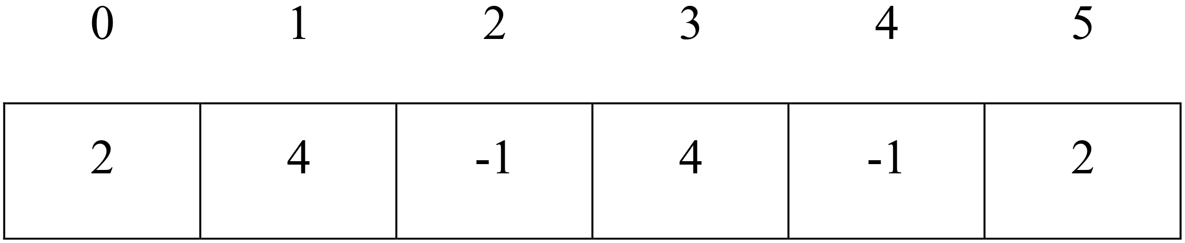

For example, if we want to represent a partition of four data objects into two clusters, we would have a chromosome of length six, as the one depicted in Fig. 1. In this figure, the objects at indices 2 and 4 are the chosen medoids for the two clusters, the objects at indices 0 and 5 belong to the same cluster as the medoid with index 2, and objects 1 and 3 belong to the same cluster as the medoid at index 4.

5.1.2 Solution representation for the weights population

In P2, a feature weights solution is represented as an array of real values, where each feature value falls in the range [0, 1], and the sum of all feature weights is equal to 1. The length of the array is the number of feature weights in the dataset plus one, where the last index is used to store the fitness of the corresponding solution. Storing the fitness of the solution is needed to facilitate the communication between the two populations as will be explained in Section 5.5. An example of a chromosome with four feature weights in P2 is shown in Fig. 2.

Figure 2.

Example of solution representation in P2.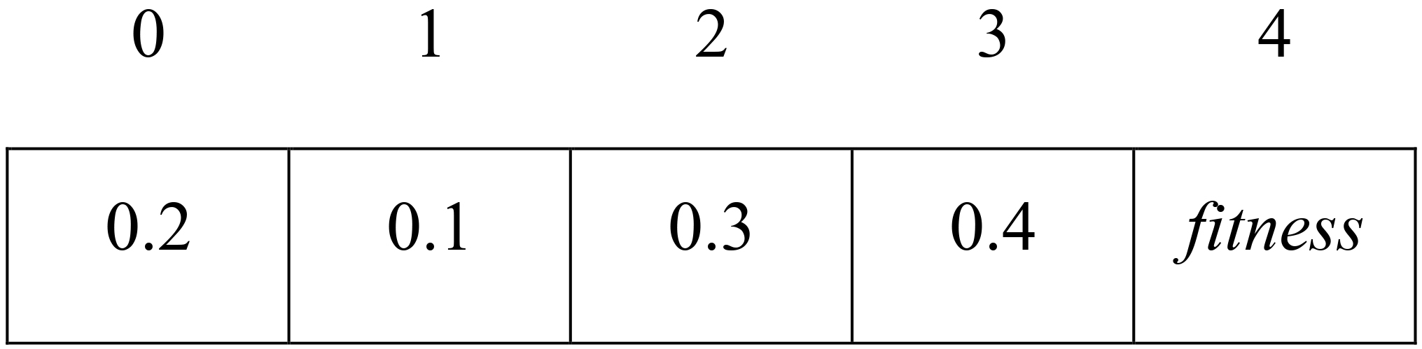

5.2 Initial population generation

5.2.1 Clustering population

The initial population is randomly generated with $K$ randomly selected clusters centers for each solution. According to [47], $K$ can be any value from the range $K_{\min}=2$ to $K_{\max}=\sqrt{N}$ , where $N$ is the size of the dataset (i.e., the number of objects to be clustered). Thus, we choose $K$ randomly within this range. After selecting the number of clusters, the medoids are selected randomly in each chromosome, and their corresponding genes are set to $-$ 1. Each data object, other than the medoids, is then assigned to its nearest medoid index. The feature weights population is not considered when generating the initial clustering population.

5.2.2 Feature weights population

The initial feature weights population is generated randomly. All the weights are real numbers between 0 included and 1 excluded, such that the sum of all feature weights is equal to 1. The fitness values of the initial weights population candidates are all set to zero initially. The first candidate in the population is set as the best weight candidate (BestWeightCandidate), which will be used to generate the second generation of the clustering population, as will be explained in Section 5.5.

5.3 Selection and replacement strategies

The selection strategy refers to the mechanism for selecting solutions to apply the genetic operators and produce new solutions. A good selection mechanism should give higher chance for fitter individuals for reproduction, but weak individuals should not be completely discarded and should also be occasionally selected [20]. In our algorithm we use a Roulette-Wheel selection mechanism [32], where each individual is selected based on a probability that is proportionate to its fitness; i.e., fitter individuals have larger slices in the ‘roulette wheel’ and thus have higher chance of being selected.

To choose the individuals surviving to the next generation between the old population and the new population generated after reproduction, we use an elitism strategy, where a certain number of best individuals is preserved from the old population and migrated with the new population.

5.4 Genetic operators

Our co-evolutionary approach relies on mutation operators only for evolving both P1 and P2. Initial experimentation with a Join and Split (J&S) crossover [2]for the clustering population indicated degradation in performance when this operator is used, as compared to when using mutation only. Therefore, it was discarded in the final tested version of the algorithm.

5.4.1 Mutation in P1

A cluster oriented mutation operator is applied to all selected candidates returned from the selection strategy [2]. The mutation operator consists of randomly determining whether to add or remove a cluster center from each candidate solution, while respecting the limits on the number of clusters. In both cases, reassigning objects according to the new cluster centers will be performed. When reassigning objects, the BestWeightCandidate (i.e., the fittest individual in P2) will be considered while calculating the distances.

5.4.2 Mutation in P2

Every candidate in P2 will be mutated by randomly selecting two feature weights from the chromosome $w_{1}$ and $w_{2}$ . Then, we subtract a random value $\varepsilon$ ( $0<=\varepsilon<=w_{1}$ ) from $w_{1}$ and add it to $w_{2}$ , maintaining that no feature will have a weight smaller than 0 or greater than 1, and the sum of all the feature weights is equal to 1 [2]. The value of $\varepsilon$ falls in the range $[0,w_{1}]$ .

5.5 Coevolution process

In our approach, we apply a cooperative co-evolutionary algorithm on two populations, where the fitness of a candidate in one population is affected by the quality of other candidates from the other population [68]. As the name implies, these two populations work together in cooperative way to solve a problem, where each population has a role in the evaluation of the overall objective function [65]. In what follows, we explain the proposed approach, in terms of the evaluation of the fitness scores, and how the evolution from one generation to the next proceeds in the two populations.

5.5.1 Fitness scores

1) Clustering population

The clustering population will consider the BestWeightCandidate (i.e., the fittest individual in the weights population) when evaluating its candidates using the $\frac{BC}{WC}$ ratio discussed in Section 4.

2) Feature weights population

To calculate the fitness of each individual in the weights population, a candidate is evaluated with all candidates in the clustering population using the $\frac{BC}{WC}$ ratio (Eq. (8)). When the evaluation ends, the fitness score of the current feature weights candidate is set to the same fitness score attached to the clustering candidate that returned the highest $\frac{BC}{WC}$ ratio. The fitness score is then stored in the last index of the chromosome as explained in Section 5.1, since it is needed to determine the BestWeightCandidate later on. This process is repeated for the entire feature weights population.

After the population is evaluated and updated with fitness scores, the BestWeightCandidate is set to the weight candidate with the highest fitness score.

Figure 3 illustrates the evaluation process of the clustering population, and Fig. 4 illustrates the evaluation process of the weights population.

Figure 3.

Clustering population evaluation.

Figure 4.

Weight population evaluation.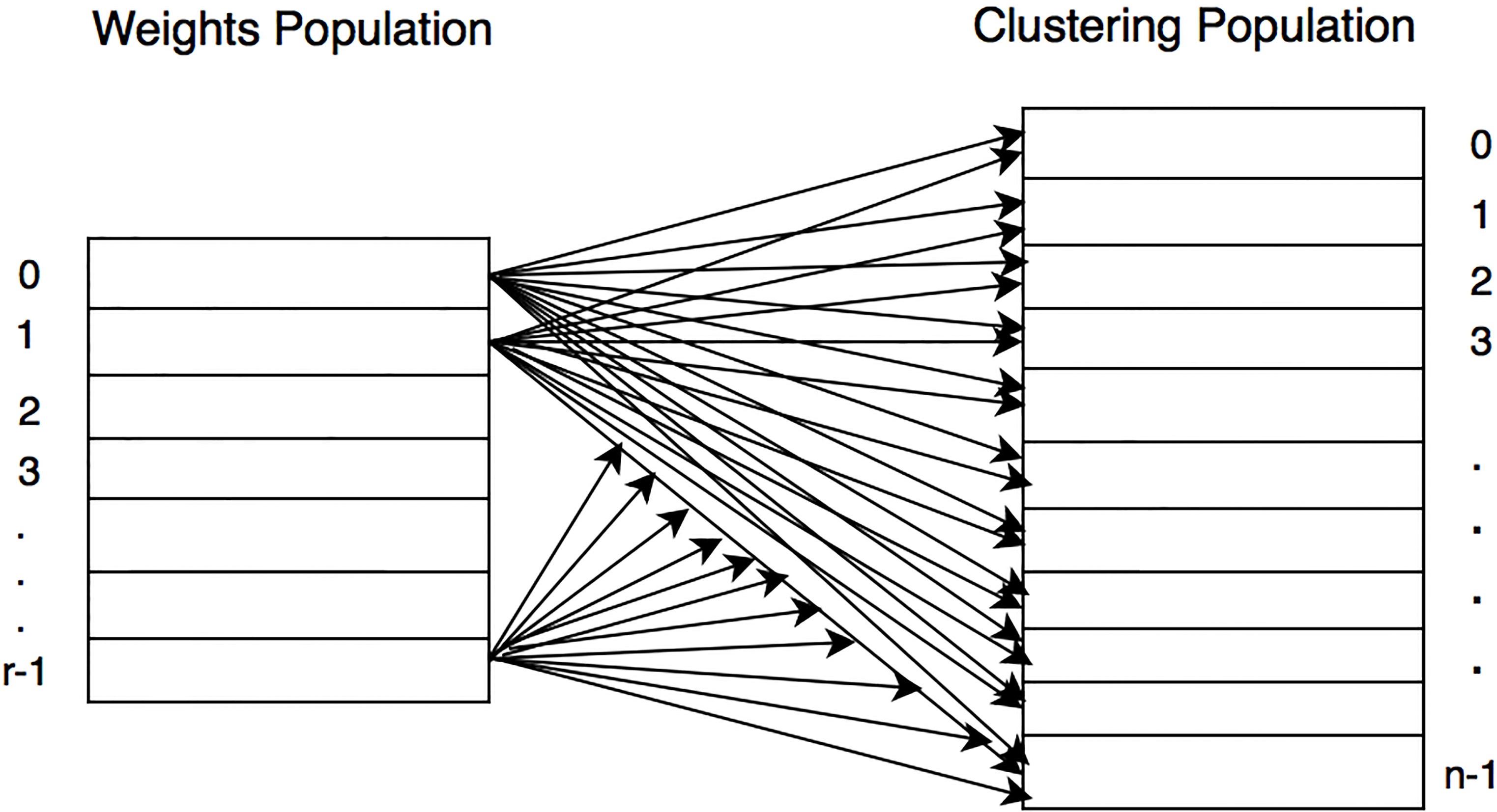

Figure 5.

Serial (sequential) co-evolution.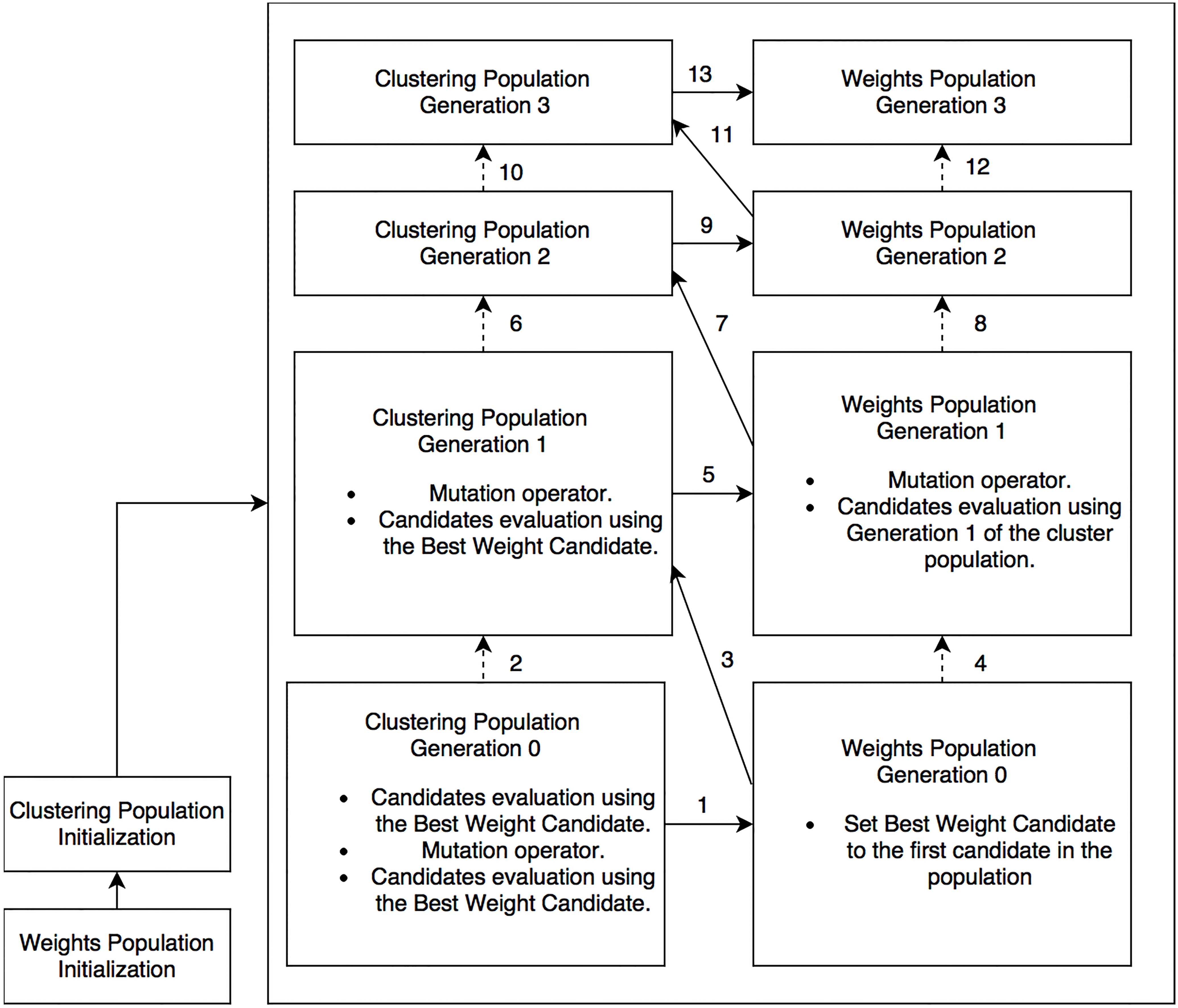

5.5.2 The co-evolution of the two populations

Figure 5 illustrates the co-evolutionary process and the order of evolving the two populations based on the sequential coevolution mechanism described in [45].

A Pseudocode of the algorithm used is shown in Algorithm 3. The algorithm consists of two phases: initialization phase and coevolution phase. The initialization phase starts by reading the data and constructing a lookup table [39] that is intended to reduce the processing time. The lookup table is a matrix, where the distances between all pairs of objects are saved in advance (ignoring the feature weights in the Euclidean distance formula (Eq. (7)). Therefore, these distances are calculated only once throughout the whole evolutionary process. After initializing the two populations, the coevolution phase then proceeds by alternating the mutation operators and the evaluation between the two populations as illustrated in Fig. 5.

Algorithm 3: Pseudocode of the co-evolutionary algorithm
BEGIN//initialization Phase
1. Read Dataset 2. Construct Lookup Table //Generate feature weights population 3. WHILE numOfFeaturesWeightsCandidates $<$ FeaturesWeightsPopulationSize – Generate newWeightCandiadte with random values in the range [0,1) such that the sum of all the feature weights is equal to 1 – Set the fitness score of the newCandidate to zero END WHILE 4. Set BestWeightCandidate to the first candidate in FeaturesWeightsPopulation //Generate Clustering population 5. WHILE numOfClusterCandidates $<$ ClusterPopulationSize – Generate newClusterCandiadte by randomly selecting $K$ cluster centers from the dataset objects, such that $2\leqslant K\leqslant\quad\sqrt{N}$ , where $N$ is the size of the dataset – FOR each object in the dataset that is not a cluster center * Assign the object to the nearest cluster center END FOR END WHILE 6. FOR each Candidate in the ClusterPopulation – Use the BestWeightCandidate to calculate the ClusterCandidate fitness score by applying the $\frac{BC}{WC}$ ratio END FOR 7. BestSoFarClusterCandidate $=$ null 8. BestSoFarFeaturesWeightsCandidate $=$ null //Coevolution Phase
REPEAT
1. Select ClusterPopulationSelectedCandidates from the Cluster Population using RouletteWheel selection 2. FOR each Candidate in the ClusterPopulationSelectedCandidates – Apply a Cluster Oriented Mutation Operator – Reassign objects to their nearest cluster END FOR 3. FOR each Candidate in the ClusterPopulation – Use the BestFeaturesWeightsCandidate to calculate the ClusterCandidate Fitness score by applying the $\frac{BC}{WC}$ ratio END FOR 4. Set the BestClusterCandidate to the ClusterCandidate with the highest Fitness score 5. FOR each FeaturesWeightsCandidate in the FeaturesWeightsPopulation – Apply Weight Population Mutation Operator – FOR each ClusterCandidate in the ClusterPopulation * Evaluate the FeaturesWeightsCandidate with this ClusterCandidate using $\frac{BC}{WC}$ ratio END FOR – Set the FeaturesWeightsCandidate Fitness score to the Fitness score of the ClusterCandidate that returned the highest Fitness score. END FOR 6. Set BestFeaturesWeightsCandidate to the FeaturesWeightsCandidate with the highest Fitness score. 7. IF BestSoFarClusterCandidate Fitness $<$ BestClusterCandidate Fitness – Set BestSoFarClusterCandidate to BestClusterCandidate END IF 8. IF BestSoFarFeaturesWeightsCandidate Fitness $<$ BestFeaturesWeightsCandidate Fitness – Set BestSoFarFeaturesWeightsCandidate to BestFeaturesWeightsCandidate END IF UNTIL numberOfGenerations $=$ maxGenerationsEnd

6. Computational experimentation

The algorithm was implemented on MacBook Air, 1.4 GHz Intel Core i5 processor, and 4 GB 1600 MHz DDR3 Memory, with OS X version 10.9.5. To implement the evolutionary components, we used Watchmaker Framework version 0.7.1 [11], which is an object-oriented framework for developing evolutionary algorithms in Java. We integrated it with JGrasp version 2.0.1_01 and used it to implement the various components of our co-evolutionary algorithm.

Before testing the algorithm, several parameters must be set, such as the population size, crossover and mutation rates, number of generations, etc. To set these parameters we used both recommendations from previous literature as well as some preliminary testing of different values, aiming to obtain a balance between processing time and solution quality. For each parameter, we tried several values while maintaining all other parameters unchanged. When we decide on a value, we move on to the next parameter. For the population size, 50, 100 and 200 were evaluated. The elitism rate (i.e., number of fittest candidates that survive to the next generation) was tested with the values: 5, 10, and 20. For the termination condition we tested stagnation with 20, 30, 40, 50, and 70 generation, versus running the evolutionary process for a fixed number of generations set to 100 and 200. A Split & Join crossover [2] and our mutation operators have been evaluated with different probabilities in the range [0, 1].

After these experiments, the clustering population size has been set to 100; the mutation operator probability was set to 1; the Split & Join crossover was discarded due to degradation in performance when this operator was used; the elitism rate was set to 10; the termination condition has been decided as terminating the evolutionary process after a fixed number of generations have passed. We have set the maximum number of generations to 200 as in [25]. To speedup the co-evolutionary process, especially when evaluating the weights population fitness, the size of the weights population has been set to only 5.

6.1 Comparing weights adaptation against non-adaptive weights

To evaluate our co-evolutionary algorithm we tested it against another version of the algorithm, where the feature weights are not adapted and not evolved during the search. In other words, in this version of the algorithm, we only have one population, which is the clustering population that is optimized during the search. The same parameters and the same cluster oriented mutation operator (explained in Section 5.4) are used to optimize the clustering solution. In addition, the fitness function in this version uses the $\frac{BC}{WC}$ ratio, while ignoring the weights of the features in calculating the distances between the objects.

We used the University of California Irvine (UCI) Machine Learning Repository [37] to test our approach. We selected three datasets that are commonly used for testing clustering to run the experiments: The Iris dataset, the Wine dataset, and the Seeds dataset. Each version of the algorithm was run 30 times and the best and average cluster quality values were measured using the $\frac{BC}{WC}$ ratio. In each run, the best individual encountered throughout the evolutionary process is returned as the solution for this run.

Table 1 shows the results on the Iris dataset having size $N=$ 150, and number of attributes $=$ 4. The table shows the results for both implemented versions, where the first version is the co-evolutionary algorithm for the adaptation of feature weights, and the second is the standard evolutionary algorithm without weights adaptation. The table presents, for each version, the average, maximum, and minimum fitness values for the best candidate in the 30 runs, where the best-achieved fitness is highlighted in bold. In addition, the processing time in seconds is shown for both versions. The last column in the table (Gap%) indicates the percent difference between the results obtained by the version of the algorithm that does not include weights adaptation to the results obtained with the adaptation of weights.

Table 1
Results on the Iris dataset

With weights adaptation				Without weights adaptation
Result	Best cluster	# of clusters in	Proc time	Result	Best cluster	# of clusters in	Proc time	Gap%
	fitness	best candidate	(Sec)		fitness	best candidate	(Sec)
Average	651.96	11.53	2.03	Average	270.72	11.87	1.07	58%
Maximum	895.26	12.00	3.00	Maximum	357.11	12.00	2.00	60%
Minimum	360.31	10.00	2.00	Minimum	223.90	11.00	1.00	38%

Table 1 clearly indicates that the results obtained with weights adaptation are greatly superior to the results of the version that does not involve the utilization of feature weights. This is evident by the large gap percent to the best results as indicated in the last column of the table. The last column shows that the adaptation of weights has improved the best fitness by 60% and the average fitness by 58%. Also, the minimum fitness value has been improved by 38%. Both versions of the algorithm were able to achieve comparable number of clusters, ranging between 10–12 clusters in the best candidate. Regarding the processing time, both versions are very quick with time not exceeding 2–3 seconds for each run. However, the version having the weights adaptation takes slightly more processing time than the other version. The average obtained feature weights for the best weight candidate in the 30 runs were: (0.070, 0.095, 0.679, 0.156), for the four features of the Iris dataset (sepal length, sepal width, petal length and petal width, respectively), indicating that that petal dimensions (shown in bold) are more important for clustering than sepal dimensions, from the perspective of our co-evolutionary algorithm.

Figure 6 compares the average fitness value for the best candidates obtained throughout the evolutionary process (i.e., during 200 generations) in each run, for both tested versions of the algorithm. It is clear from the figure that the weights adaptation version consistently produces better average fitness in all runs (except in two runs where the average fitness values were the same).

In addition, to further validate the stability of our algorithm, we have computed the 95% confidence interval of both versions of the algorithm for the Iris dataset. Regarding the best cluster fitness, the 95% confidence interval is [596.90, 707.03] for the version having the adaptation of weights compared to [258.38, 283.05] for the version without weights adaptation, which shows beyond doubt the significant difference between the performance of the two algorithms in terms of achieving better cluster fitness values. On the other hand, regarding the number of clusters in the best candidate, the 95% confidence interval for the weights adaptation version was [11.29, 11.78] compared to [11.74, 11.99] for the version with the non-adaptive weights, which indicates a comparable performance in terms of the number of clusters in both versions, since this part of the optimization process is in fact identical in both versions and is not directly related to the adaptation of weights.

Table 2

Results on the Seeds dataset

With weights adaptation				Without weights adaptation
Result	Best cluster	# of clusters in	Proc time	Result	Best cluster	# of clusters in	Proc time	Gap%
	fitness	best candidate	(Sec)		fitness	best candidate	(Sec)
Average	609.00	13.67	3.43	Average	189.02	13.80	2.00	69%
Maximum	1010.90	14.00	4.00	Maximum	228.30	14.00	2.00	77%
Minimum	315.08	11.00	2.00	Minimum	159.87	13.00	2.00	49%

Figure 6.

Average fitness of all best candidates in each generation on Iris dataset.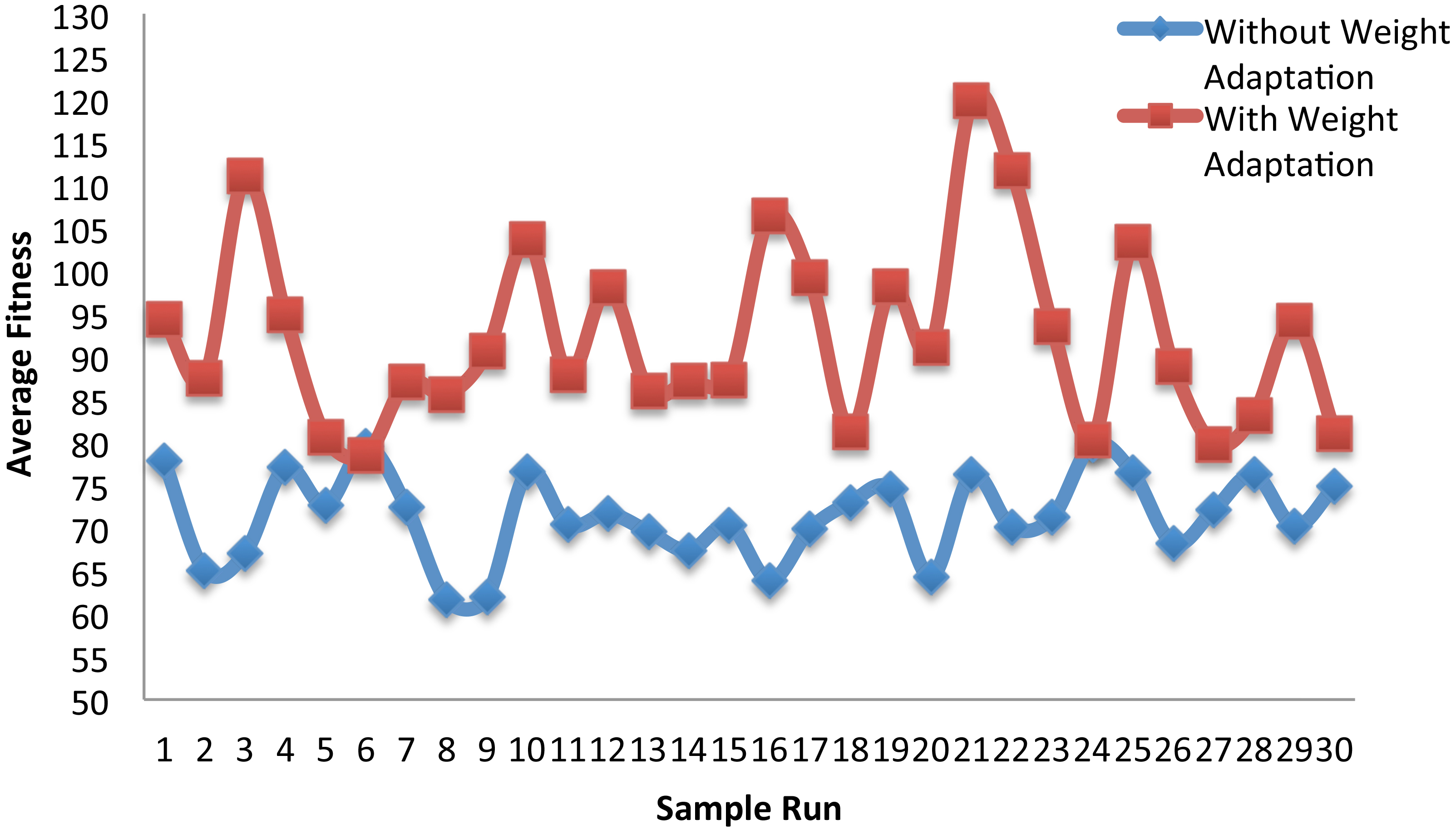

Table 2 shows the results of testing both versions of the algorithm on the Seeds dataset for 30 runs, indicating the same information as Table 1. The Seeds dataset consists of 210 objects and 7 attributes. Again the results in Table 2 show the favorable performance of the weights adaptation version as compared to clustering without adaptation of feature weights. Here the best result has been improved by an impressing 77% value when feature weights have been adapted during the search. Average and minimum fitness values have also been highly improved. For the number of clusters, both versions obtained comparable numbers ranging from 11 to 14. The processing time was again comparable, while being slightly in favor of the version that excludes the weights adaptation.

Figure 7 shows the best fitness in each run for both versions of the algorithm. Again this figure confirms that the weights adaptation version is able to consistently achieve better results, as compared to the version without weights adaptation, which is obviously stuck in a local optimum in each run.

For the Seeds dataset, the feature weights of the best candidates for all 30 runs for the 7 features were optimized as having the following average values (0.329, 0.128, 0.182, 0.102, 0.115, 0.037, 0.107). These attributes describe a wheat kernel in terms of respectively: area, perimeter, compactness, length of kernel, width of kernel, asymmetry coefficient, and length of kernel groove. As indicated by the weights highlighted in bold, our algorithm has given more importance in classification to the first attribute (i.e., the area) compared to the other attributes, while the least important feature was considered as the asymmetry coefficient.

Similar to the results on the Iris dataset, the 95% confidence intervals for both versions of the algorithm on the seeds dataset show a significant difference between their performances. The confidence interval for the weights adaptation version in terms of the best fitness was calculated as [555.81, 662.20] compared to [183.26, 194.78] for the version without weights adaptation, indicating a much favorable performance for the adaptation of weights version. Again in terms of the number of clusters, both versions had comparable performance with confidence intervals as [13.43, 13.90] and [13.65, 13.95] respectively.

The third experiment was done on the Wine dataset, which includes 178 objects and 12 attributes (excluding the class identifier, i.e., the first attribute in the dataset). Table 3 summarizes the results obtained after running the two versions of the algorithm 30 times each.

Table 3

Results on the Wine dataset

With weights adaptation				Without weights adaptation
Result	Best cluster	# of clusters in	Proc time	Result	Best cluster	# of clusters in	Proc time	Gap%
	fitness	best candidate	(Sec)		fitness	best candidate	(Sec)
Average	225.45	12.47	2.70	Average	156.24	12.40	1.03	31%
Maximum	432.88	13.00	3.00	Maximum	197.64	13.00	2.00	54%
Minimum	92.69	10.00	2.00	Minimum	118.08	9.00	1.00	27%

Figure 7.

Best fitness in each run on the Seeds dataset.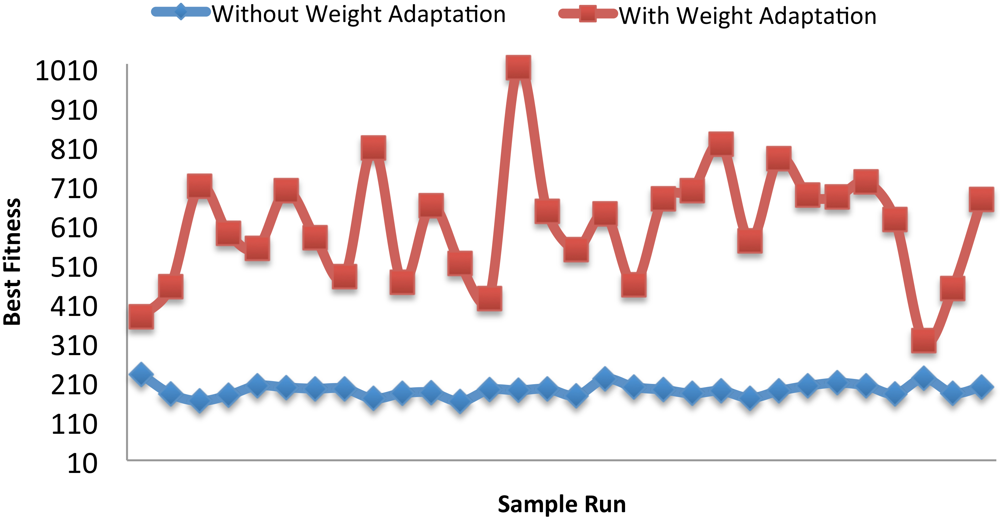

Similar to Tables 1 and 2, the results in Table 3 indicate that the adaptation of feature weights has improved the best fitness by 54%, compared to when feature weights are ignored. Also, the average fitness has improved by 31% and minimum fitness has improved by 27%. The achieved number of clusters ranged from 9–13 in both versions. Again the processing time was slightly in favor of the version that does not have weights adaptation. The average feature weights for best candidates in the 30 runs were calculated by the evolutionary process as follows: (0.055, 0.049, 0.107, 0.042, 0.164, 0.055, 0.085, 0.075, 0.088, 0.090, 0.106, 0.084), which indicates more weights were given for the 3 ${}^{\text{rd}}$ , 5 ${}^{\text{th}}$ , and the 11 ${}^{\text{th}}$ attributes in the features set, compared to other attributes.

Figure 8.

Best fitness in each run on the Wine dataset.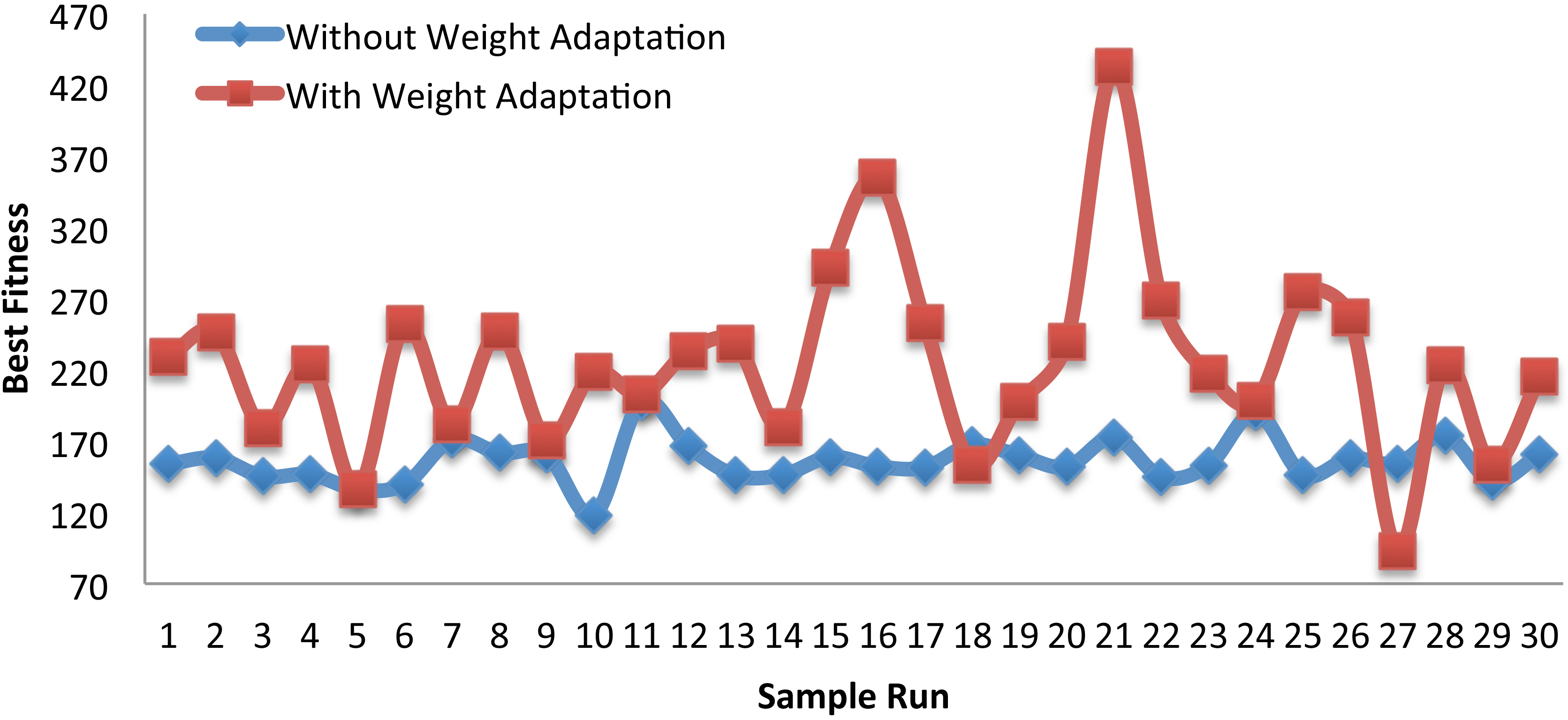

Figure 8 shows a comparison between the different runs performed by both versions of the algorithm on the Wine dataset in terms of the best fitness value in each run. As the figure indicates, in all except three runs, the weights adaptation version was able to produce better solutions than the solutions obtained by the version without weights adaptation.

To conclude this experiment, the 95% confidence interval for the wine dataset was calculated as [202.47, 248.43] for the fitness obtained in the adaptation of weights version of the algorithm, compared to [150.65, 161.83] for the second version having fixed weights. Again this shows the ability of the weights adaptation version to significantly outperform the other version in terms of the best fitness value. On the other hand, for the number of clusters both intervals were comparable with [12.21, 12.73] and [12.03, 12.77] respectively for the two versions.

6.2 Comparing against the K-means with fixed number of clusters

The next experiment that was conducted to validate our approach was testing the performance of the algorithm against the K-means clustering algorithm using a fixed number of clusters. In other words, we assumed here that the number of clusters is known a priori in order to test whether the algorithm in this case will be able to classify the instances correctly in the clusters categories that are pre-determined in the dataset. For this purpose we tested the algorithm again on the Iris dataset by fixing the number of clusters to three, which is the original number of clusters known for the Iris dataset. To do the mutation, each time only one cluster was selected at random and changed to another cluster. The rest of the co-evolutionary process and the parameters used were not changed than the previous version. The algorithm was run 10 times in this experiment. To obtain the results of the K-means algorithm we ran it on the WEKA tool [22]. Table 4 shows the results obtained by our algorithm in the 10 runs in terms of the number of misclassified instances.

Table 4
Results with a fixed number of clusters on the Iris dataset

Run	No of misclassified instances
1	15
2	10
3	7
4	14
5	20
6	17
7	12
8	6
9	34
10	6

In comparison, the results obtained by the K-means algorithm were 17 misclassified instances, i.e., 11.33% misclassified instances over the 150 instances of the Iris dataset. As Table 4 indicates, our approach was able to obtain similar or better result than K-means in 8 out of 10 runs (shown in boldface). The best result obtained by our algorithm had only 6 misclassified instances, i.e., an approximately 65% improvement over K-means result, and with only 4% of instances being misclassified.

6.3 Comparing against subspace clustering

The final experiment that we did to validate our approach was making a comparison between the results obtained by our algorithm and the subspace co-evolutionary clustering approach of [16]. We compared the results of the LC-LKM approach reported in [16], since it is the approach that is closest to our method among the two tested methods in this paper. Specifically LC-LKM uses a distance-based function to define non-overlapping clusters, similar to what is done in our method. For the sake of this comparison, we ran the algorithm on the three data sets that are used in [16]: the Iris data set, the Pima Indians Diabetes data set, and the Ionosphere dataset. As in [16], we ran the algorithm100 times with a fixed number of clusters (i.e., similar to what was done in our last experiment reported in Section 6.2). We then calculated the average R-index [21] obtained by our algorithm and compared it with the average R-index of the LC-LKM algorithm of [16]. The results obtained for the Iris data set was an average R-index of 0.88 which is similar to the R-index value of approximately 0.9 reported in [16]. Moreover, the maximum R-index of the 100 runs obtained by our algorithm was 0.95 for the Iris data set. For the Pima Indians Diabetes data set, we obtained an average R-index of 0.55 which is slightly better than the average of the LC-LKM subspace clustering in [16] (approximately 0.5). The best R-index value in the 100 runs obtained by our algorithm was 0.62 for the Pima Indians Diabetes data set. Finally, for the Ionosphere data set our average R-index is 0.54, which is slightly less than the average obtained by [16] (approximately 0.62). Overall, these results prove that our algorithm is able to achieve comparable performance to the subspace clustering, while having the advantage of requiring less information about the dimensionality of each subspace.

7. Conclusions and future research

Data clustering is the process of dividing a dataset into groups of objects with similar characteristics, such that the within group similarity is maximized compared to the between groups similarity. Data clustering has many applications in data mining and machine learning fields. However, today’s data, especially that is involved in the World Wide Web’s applications, is very complex and multi-dimensional in nature. This indeed complicates the clustering process and affects its efficiency. With lack of domain knowledge regarding the most relevant or important features for data clustering, unsupervised learning of relevant feature weights becomes an attractive solution for difficult clustering problems. In this paper, we proposed a co-evolutionary algorithm for multi-dimensional clustering, where the clustering process together with the adaptation of feature weights are done simultaneously in a co-operative manner. In addition, the number of clusters is not known a priori; rather, it is also learnt and optimized in the evolutionary process.

To test our proposed approach, we have done multiple experiments on datasets obtained from UCI machine learning repository. The results were compared with another version of the algorithm that performs evolutionary clustering without adaptation of feature weights. The experimental results indicate the efficiency of the proposed approach, since it was able to significantly outperform the non-adaptive version for all tested datasets, and with a high level of confidence. In addition, when compared to K-means clustering for a fixed number of clusters, our approach was able to obtain better results, in terms of the number of misclassified instances in 80% of the runs. Comparing the algorithm with subspace clustering also revealed that it produces comparable results in terms of the achieved clustering accuracy. These results indicate that our proposed approach is very robust and able to efficiently perform the clustering task for different datasets with high dimensionality. This technique is especially beneficial when no or very little domain knowledge is available regarding the number of clusters, and the relevance level or the importance of the underlying feature weights. It should be noted, though, that the interpretation of the results obtained by our co-evolutionary method might need a domain expert in the field, in order to reach interesting findings that could be useful in practical scenarios.

Further research directions include testing the approach with other evolutionary operators, such as different crossover operators or other types of mutation. In addition, the approach can be further tested on higher dimensional and more complex data, such as social media data, to assess its performance for even more challenging clustering applications. Further investigation of the automatic detection of the number of clusters is also worth attention, in order to obtain a number of clusters that may be closer to the ground truth.

Footnotes

Acknowledgments

This research project was supported by a grant from the “Research Center of the Female Scientific and Medical Colleges”, Deanship of Scientific Research, King Saud University. The authors would like to thank the two anonymous referees for their valuable comments and suggestions, which have improved both the content and the presentation of the paper.

References

Agustı

L.E.

Salcedo-Sanz

Jiménez-Fernández

Carro-Calvo

Del Ser

and Portilla-Figueras

J.A.

, A new grouping genetic algorithm for clustering problems, Expert Syst. Appl 39 (2012), 9695–9703.

Al-malak

and Hosny

, A Multimodal Adaptive Genetic Clustering Algorithm, in: Proc. Genet. Evol. Comput. Conf. (GECCO 2016), ACM, Denver, Colorado, 2016.

Bandyopadhyay

and Maulik

, An evolutionary technique based on K-means algorithm for optimal clustering in RN, Inf. Sci. 146(n.d.) (2002), 221–237.

Bezdek

Boggavarapu

Hall

and Bensaid

, Genetic algorithm guided clustering, in: IEEE World Congr. Comput. Intell, 1994, pp. 34–39.

Chatzilari

Nikolopoulos

and Patras

, Enhancing computer vision using the collective intelligence of social media, in: New Dir. Web Data Manag. 1, Springer Berlin Heidelberg, 2011, pp. 235–271.

Cole

, Clustering with genetic algorithms, Citeseer, 1998.

Dash

and Liu

, Feature Selection for Clustering, in: Knowl. Discov. Data Mining. Curr. Issues New Appl, Springer Berlin Heidelberg, 2000, pp. 110–121.

DeSarbo

Carroll

Clark

and Green

, Synthesized clustering: A method for amalgamating alternative clustering bases with differential weighting of variables, Psychometrika 49 (1984), 57–78.

Dorigo

, Optimization, learning and natural algorithms, Ph. D. Thesis, Politecnico di Milano, Italy, 1992.

10.

, Data mining techniques and applications: An introduction, Cengage Learning, 2010.

11.

Dyer

D.W.

, Watchmaker framework for evolutionary computation, 2006.

12.

Estivill-Castro

and Murray

, Spatial clustering for data mining with genetic algorithms, Queensland University of Technology, Australia, 1997.

13.

Falkenauer

, Genetic algorithms and grouping problems, John Wiley & Sons, Inc., 1998.

14.

Fränti

Kivijärvi

Kaukoranta

and Nevalainen

, Genetic algorithms for large-scale clustering problems, Comput. J. 40 (1997), 547–554.

15.

Freitas

, Data mining and knowledge discovery with evolutionary algorithms, Springer Science & Business Media, 2013.

16.

Gançarski

Blansche

and Wania

, Comparison between two coevolutionary feature weighting algorithms in clustering, Pattern Recognit 41 (2008), 983–994.

17.

Giannakidou

and Kompatsiaris

, Semsoc: Semantic, social and content-based clustering in multimedia collaborative tagging systems, in: Semant. Comput. 2008 IEEE Int. Conf., 2008.

18.

Gnanadesikan

Kettenring

and Tsao

, Weighting and selection of variables for cluster analysis, J. Classif. 12 (1995), 113–136.

19.

Goldberg

D.E.

, Genetic algorithms in search, optimization, and machine learning, Addion wesley, 1989.

20.

Goldberg

D.E.

and Deb

, A comparative analysis of selection schemes used in genetic algorithms., Found. Genet. Algorithms 1 (1991), 69–93.

21.

Halkidi

Batistakis

and Vazirgiannis

, On Clustering Validation Techniques, J. Intell. Inf. Syst 17 (2001), 107–145.

22.

Hall

Frank

Holmes

Pfahringer

Reutemann

and Witten

I.H.

, The WEKA data mining software: an update, ACM SIGKDD Explor. Newsl 11 (2009), 10–18.

23.

Han

Karypis

and Kumar

, Text categorization using weight adjusted k-nearest neighbor classification, in: Pacific-Asia Conf. Knowl. Discov. Data Min, Springer Berlin Heidelberg, 2001.

24.

Hansen

and Jaumard

, Cluster analysis and mathematical programming, Math. Program 79 (1997), 191–215.

25.

and Tan

, A two-stage genetic algorithm for automatic clustering, Neurocomputing 81 (2012), 49–59.

26.

Hruschka

Campello

and Freitas

A.A.

, A survey of evolutionary algorithms for clustering, IEEE Trans. Syst. Man, Cybern. Part C (Applications Rev.) 39 (2009), 133–155.

27.

Hruschka

and de Castro

, Evolutionary algorithms for clustering gene-expression data, in: Data Mining, 2004. ICDM’04. Fourth IEEE Int. Conf., IEEE, 2004, pp. 403–406.

28.

Hruschka

and Ebecken

, A genetic algorithm for cluster analysis, Intell. Data Anal 7 (2003), 15–25.

29.

Hruschka

E.R.

Campello

R.J.G.B.

Freitas

A.A.

and de Carvalho

A.C.P.L.F.

, A survey of evolutionary algorithms for clustering, IEEE Trans. Syst. Man Cybern. Part C Appl. Rev. 39 (2009), 133–155.

30.

Jain

and Dubes

, Algorithms for clustering data, Prentice-Hall, Inc., Englewood Cliffs, NJ, 1988.

31.

Jain

A.K.

Murty

M.N.

and Flynn

P.J.

, Data Clustering: A Review, ACM Comput. Surv 31 (1999), 264–323.

32.

De Jong

K.A.

, An analysis of the behavior of a class of genetic adaptive systems, University of Michigan, 1975.

33.

Kogan

Nicholas

Teboulle

et al., A Survey of Clustering Data Mining Techniques, in: Group. Multidimens. Data, Springer Berlin Heidelberg, 2006, pp. 25–71.

34.

Krishna

and Murty

, Genetic K-means algorithm, IEEE Trans. Syst. Man, Cybern. Part B. 29 (1999), 433–439.

35.

Krovi

, Genetic algorithms for clustering: a preliminary investigation, in: Syst. Sci. 1992. Proc. Twenty-Fifth Hawaii Int. Conf., IEEE, Hawaii, 1992, pp. 540–544.

36.

Kuncheva

and Bezdek

, Selection of cluster prototypes from data by a genetic algorithm, in: 5th Eur. Congr. Intell. Tech. Soft Comput, 1997, pp. 1683–1688.

37.

Lichman

, UCI Machine Learning Repository, 2013.

38.

Lienhart

Romberg

and Hörster

, Multilayer pLSA for multimodal image retrieval, in: Proc. ACM Int. Conf. Image Video Retr, 2009, p. 9.

39.

Lin

Yang

and Kao

, An efficient GA-based clustering technique, Tamkang J. Sci 8 (2005), 113–122.

40.

Liu

and Yu

, Toward integrating feature selection algorithms for classification and clustering, IEEE Trans. Knowl. Data Eng 17 (2005), 491–502.

41.

Liu

and Shen

, Automatic clustering using genetic algorithms, Appl. Math. Comput 218 (2011), 1267–1279.

42.

Fotouhi

Deng

and Brown

S.J.

, Incremental genetic K-means algorithm and its application in gene expression data analysis, Bioinformatics (2004).

43.

Fotouhi

Deng

and Brown

, FGKA: A fast genetic k-means clustering algorithm, in: Proc. 2004 ACM Symp. Appl. Comput, 2004, pp. 622–623.

44.

Lucasius

Dane

and Kateman

, On k-medoid clustering of large data sets with the aid of a genetic algorithm: background, feasiblity and comparison, Anal. Chim. Acta 282 (1993), 647–669.

45.

Luke

, Essentials of Metaheuristics, second, Lulu, 2013.

46.

Chan

Yao

and Chiu

D.K.

, An evolutionary clustering algorithm for gene expression microarray data analysis, IEEE Trans. Evol. Comput 10 (2006), 296–314.

47.

Mardia

K.V.

Kent

J.T.

and Bibby

J.M.

, Multivariate Analysis, Analysis 97 (1979), 1–4.

48.

Merz

and Zell

, Clustering gene expression profiles with memetic algorithms, in: Int. Conf. Parallel Probl. Solving from Nat, Springer Berlin Heidelberg, 2002, pp. 811–820.

49.

Modha

and Spangler

, Feature weighting in k-means clustering, Mach. Learn 52 (2003), 217–237.

50.

Molina

L.C.

Belanche

and Nebot

, Feature selection algorithms: a survey and experimental evaluation, in: 2002 IEEE Int. Conf. Data Mining, 2002. Proceedings, IEEE Comput. Soc, 2002, pp. 306–313.

51.

Murthy

and Chowdhury

, In search of optimal clusters using genetic algorithms, Pattern Recognit. Lett 17 (1996), 825–832.

52.

Naldi

, Clustering using genetic algorithm combining validation criteria., in: ESANN, 2007, pp. 139–144.

53.

Neha

and Vidyavathi

, A Survey on Applications of Data Mining using Clustering Techniques, Int. J. Comput. Appl 126 (2015).

54.

Nikolopoulos

Giannakidou

and Kompatsiaris

, Combining multi-modal features for social media analysis, in: Hoi

S.C.H.

Luo

Boll

Jin

King

, eds, Soc. Media Model, Springer, 2011, pp. 71–96.

55.

Parsons

Haque

and Liu

, Subspace clustering for high dimensional data: a review, ACM SIGKDD Explor. Newsl 6 (2004), 90–105.

56.

Pena

Lozano

and Larranaga

, An empirical comparison of four initialization methods for the k-means algorithm, Pattern Recognit. Lett 20 (1999), 1027–1040.

57.

Piatrik

and Izquierdo

, Subspace clustering of images using ant colony optimisation, in: 2009 16th IEEE Int. Conf. Image Process, IEEE, 2009, pp. 229–232.

58.

Rai

and Singh

, A Survey of Clustering Techniques, Int. J. Comput. Appl 7 (2010), 1–5.

59.

Scheunders

, A genetic c-means clustering algorithm applied to color image quantization, Pattern Recognit 30 (1997), 859–866.

60.

Shankar

and Karypis

, Weight adjustment schemes for a centroid based classifier, 2000.

61.

Sheikh

and Raghuwanshi

, Genetic algorithm based clustering: a survey, in: First Int. Conf. Emerg. Trends Eng. Technol, IEEE, 2008, pp. 314–319.

62.

Sheng

and Liu

, A hybrid algorithm for k-medoid clustering of large data sets, in: Evol. Comput. 2004. CEC2004, IEEE, 2004.

63.

De Soete

, Optimal variable weighting for ultrametric and additive tree clustering, Qual. Quant 20 (1986), 169–180.

64.

De Soete

, OVWTRE: A program for optimal variable weighting for ultrametric and additive tree fitting, J. Classif 5 (1988), 101–104.

65.

Talbi

E.G.

, Metaheuristics: from design to implementation, John Wiley & Sons, 2009.

66.

Tsai

and Chiu

, Developing a feature weight self-adjustment mechanism for a K-means clustering algorithm, Comput. Stat. Data Anal 52 (2008), 4658–4672.

67.

Wettschereck

Aha

and Mohri

, A review and empirical evaluation of feature weighting methods for a class of lazy learning algorithms, Artif. Intell. Rev. 11 (1997), 273–314.

68.

Wiegand

R.P.

, An Analysis of Cooperative Coevolutionary Algorithms, George Mason University, 2003.

69.

and Wunsch

, Survey of clustering algorithms, IEEE Trans. Neural Networks 16 (2005), 645–678.

70.

and Liu

, Efficient Feature Selection via Analysis of Relevance and Redundancy, J. Mach. Learn. Res. 5 (2004), 1205–1224.

A co-evolutionary framework for adaptive multidimensional data clustering

Abstract

Keywords

1. Introduction

2. Background

2.1 Data clustering

2.2 Traditional clustering techniques and genetic algorithm based clustering

2.2.1 Hierarchical clustering (HC)

2.2.2 Partitional clustering (PC)

2.2.4 Grid based clustering (GBC)

3.1 Genetic clustering algorithms

3.1.1 Solution representation

3.1.2 Genetic operators

3.2 Feature selection and weight optimization in multidimensional clustering

4. Problem definition

5.1 Solution representation

5.1.1 Solution representation for the clustering population

5.2.1 Clustering population

5.2.2 Feature weights population

5.3 Selection and replacement strategies

5.4 Genetic operators

5.4.1 Mutation in P1

5.4.2 Mutation in P2

5.5 Coevolution process

5.5.1 Fitness scores

1) Clustering population

2) Feature weights population

6.1 Comparing weights adaptation against non-adaptive weights

Table 1 Results on the Iris dataset

Table 4 Results with a fixed number of clusters on the Iris dataset

7. Conclusions and future research

Footnotes

Acknowledgments

References

Table 1
Results on the Iris dataset

Table 4
Results with a fixed number of clusters on the Iris dataset