Beyond accuracy – A SMART approach to site-based spatio-temporal data quality assessment

Abstract

There is a need for robust solutions to the challenges of spatio-temporal data quality assessment that include and go beyond assessment of accuracy. Emphasis is often placed on the quality assessment of individual observations from sensors but not on the sensors themselves nor upon site metadata such as location and timestamps. The focus of this paper is on the development and evaluation of such a representative, interpolation-based solution for the assessment of spatio-temporal data quality. We call our method the SMART method, short for Simple Mappings for the Approximation and Regression of Time series. A robust, linear mapping is determined between the observations from pairs of sites over a representative time period and a quadratic estimate of error is derived from these linear mappings. These mappings combine to form a robust interpolator that outperforms other popular interpolators in estimating ground truth in the presence of bad data, and that can be used to estimate ground truth and assess accuracy. The coefficients of the mappings and other derived measures can also help to identify problematic sites, including sites having incorrect location or timestamp metadata. When applied to a real-world, meteorological data set, we identify numerous problematic sites that otherwise have not been flagged as bad. We identify sites for which metadata is incorrect. We believe that there are many problems with real data sets like these and, in the absence of an approach like ours, these problems have largely gone unidentified. Our approach is novel for the simple but effective way that it accounts for spatial and temporal variation, and that it addresses more than just accuracy.

Keywords

Quality control data quality spatio-temporal data interpolation

1. Introduction

The best approach to improving the quality of sensor-data is to start at the source – the sensors – and ensure that they yield observations as close to ground truth as possible. However, it is not feasible to ensure that sensors yield ground truth at all times and under all conditions. Even if sensors are operating correctly, there are numerous potential points of failure: remote processing units (RPUs) that read data from the sensors; intermediate devices that poll the RPUs; middleware that processes sensor data; aggregators and data fusion processes that collect and redistribute the data; networks over which the data is transmitted; software that processes the data, converting it to other units or formats; custom-developed and proprietary software and hardware systems; etc. [1, 2]. And there are many data quality dimensions over which failure can occur including but not limited to accuracy, consistency, timeliness, completeness, reliability, precision [2, 3, 4].

Comparison with neighboring observations is one approach that can be taken to assess accuracy and identify problems in real time or near real time. Assuming correlation of observations having spatial and temporal proximity, we expect similarity in observation. Dissimilarity can indicate errors, i.e., differences between ground truth and observed/sensed conditions. When ground truth is not known, we are left to compare against estimates of ground truth. In making such comparisons, we find ourselves looking at slices in time, and unable to assess overall performance of individual sites. Thus, we find it useful to also compare time series from multiple, neighboring sites to assess the overall quality and fitness of an individual site/sensor.

Comparison of site-based time series becomes complicated when sites report at different times and with varying frequencies. Errors with individual observations further complicate the process when considering their adverse impact on least squares mappings, correlation coefficients, measures of covariance, etc. And if the metadata associated with a site is incorrect, then we may find ourselves comparing observations that are not in spatial or temporal proximity.

Interpolation estimates unknown values on curves or surfaces using known values. Intuitively, interpolation can be applied to assessment of accuracy by estimating ground truth at a location and comparing an observed condition to the estimate. By holding out the observed condition and interpolating at that location using neighboring observations, we can make the desired comparison. However, the errors that we seek to identify in the process of data quality assessment will have an adverse impact on interpolation.

In the absence of ground truth data, we face the challenge of attempting to identify bad data without a solid basis for comparison. As such, we may never truly know if our assessments are correct.

Our contribution: In this paper, we develop a representative, robust, interpolation-based quality assessment algorithm to determine data quality (accuracy) for site-based spatio-temporal data. We develop a representative, artificial data set which we can treat as ground truth and perturb with various types of errors for development and evaluation of our algorithm against ground truth. We then present practical extensions of this method to identify bad sites and bad metadata. We use an interpolated, raster dataset as ground truth for development and evaluation of our methods to identify bad sites and bad metadata. We apply our method to evaluate accuracy and identify bad sites and bad metadata in a prominent, real-world, atmospheric dataset. We demonstrate inconsistencies in provider quality assessment indicators for this dataset.

Scope: In this paper we present an interpolation-based method for quality control assessment of accuracy that is robust and representative, and we demonstrate the challenges of spatio-temporal data quality assessment and how to overcome these challenges. We do not present our method as a general-purpose interpolator. We extend our method to identify problematic sites. We then investigate these sites to verify that they are problematic. We do not attempt to correct erroneous data or improve collection at the source. Others state correctly that correction at the source is the best way to improve data quality [5]. Our objective is to make the most of the data from providers as-is.

Outline: The rest of this paper is organized as follows: Section 1 provides background from a real-life domain and related work, and sets the stage for our approach. SMART Mappings are presented in Section 2 and provide a foundation for the subsequent interpolator and for identifying bad sites. Section 3 presents the SMART Estimator and applies it to quality assessment (accuracy) of an artificial dataset and a real-world dataset. Section 4 applies SMART Mappings to identify bad sites and bad metadata, and presents experimental results. In Section 5, we present conclusions and future work.

Figure 1.

Air temperature near donner pass, lake tahoe and reno shown in the one-stop-shop on January 21, 2017.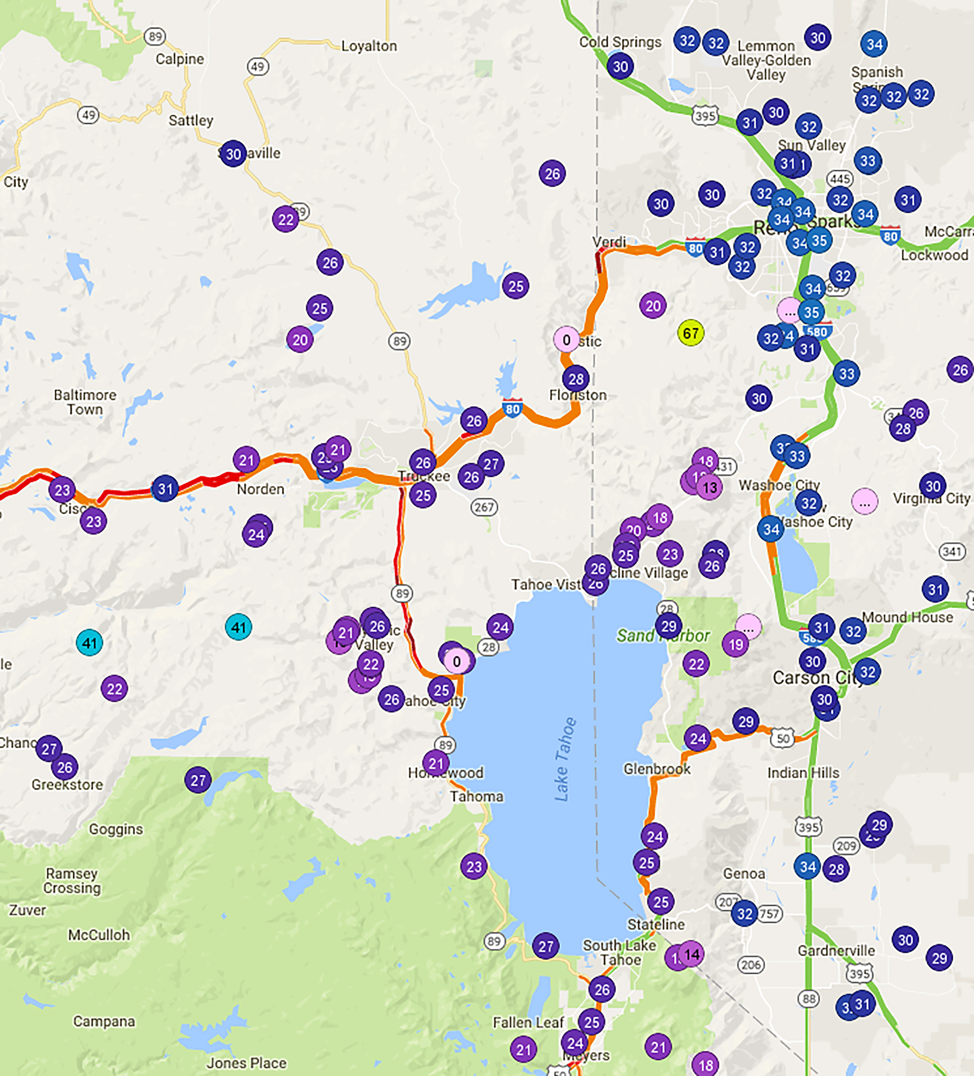

1.1 Background

Since 2003, the Western Transportation Institute (WTI) at Montana State University (MSU), in partnership with the California Department of Transportation (Caltrans), has developed web-based systems for the delivery of information from department of transportation (DOT) field elements and data from other public sources including current weather conditions and forecasts. These systems present traveler information to the traveling public and assist DOT personnel with roadway maintenance and operations. It is critical that we display quality information in these systems, yet assessing the quality of the data remains a challenge.

The WeatherShare System [6] was originally developed by WTI in partnership with Caltrans to provide a single, all-encompassing source for road weather information throughout California. Caltrans operates approximately 170 Road Weather Information Systems (RWIS) along state highways, thus their coverage is limited. It is unrealistic to expect pervasive coverage of the roadway from RWIS alone. Now in Phase 4, we are preparing the WeatherShare system to assume greater responsibility as the repository for Caltrans RWIS data. Other systems such as the One-Stop-Shop for Rural Traveler Information [7] present this information to the traveling public.

WeatherShare aggregates Caltrans RWIS data along with weather data from other third-party aggregation sources such as NOAA’s Meteorological Assimilation Data Ingest System (MADIS) [8] and the University of Utah’s MesoWest [9] to present a unified view of current weather conditions from approximately 2000 sites within California. A primary benefit of the system is far greater spatial coverage of the state, particularly roadways, relative to the Caltrans RWIS network.

In early phases of WeatherShare we implemented automated quality control procedures for identification of “bad” data with limited success. In Phase 4, we revisit this challenge. The importance of data quality for this application cannot be understated – RWIS data is used by maintenance personnel in determining how and when to treat the road to mitigate ice; it is used by operations personnel to determine when to issue warnings, chain control and when to close lanes or entire roadways; it is used by automated safety-warning systems to issue warnings to drivers; and it is used by traveler information systems that provide road-weather conditions to the traveling public. Bad data leads to bad decisions and bad decisions decrease safety.

For example, consider the temperatures shown in the Lake Tahoe/Donner Pass area including Reno in Fig. 1. Google Traffic shows slowed traffic in proximity to freezing temperatures, emphasizing the importance of correctly sensing road weather conditions. By way of color-coding, the 67 ${}^{\circ}$ F observation stands out as definitely bad. Other observations such as the two 41 ${}^{\circ}$ F readings west of Lake Tahoe appear to be erroneous, although there are observations near 40 ${}^{\circ}$ F to the west of the area shown. The two 0 ${}^{\circ}$ F observations appear questionable as well and may be indicative of a problem with those sites/sensors.

In order to assess the accuracy of data from a given site, we can use data from neighboring sites for validation. Taken in its most rudimentary form, we could simply look for anomalies on the map as we just demonstrated. Or, we could develop spatio-temporal models and compare predicted values to observed values and flag observed values as erroneous when there is a large deviation. Even if such approaches were foolproof, and we show subsequently that they are not, we have encountered little work that addresses the challenge of identifying problem sites – sites which are regularly producing erroneous data. Compounding the problem is the possibility that, like the stopped clock that is correct twice a day, sites may be producing data that is sufficiently close to that of its neighbors so-as to appear to be correct at certain times when in reality it is bad.

1.2 Literature review

The most helpful literature comes from the weather and road-weather communities and is devoted to accuracy checks for individual observations. Many of the methods are interpolation-based. The Barnes Spatial Test [10] is a variation of Inverse Distance Weighting (IDW) and has been used by the Oklahoma Mesonet [11] and the Federal Highway Administration’s Clarus project [12]. MesoWest [9] uses multivariate linear regression to assess data quality for air temperature [13, 14].

MADIS [8] implements multi-level, rule-based quality control checks [15, 16]. MADIS implements a level-3 neighbor check using Optimal Interpolation/kriging [17]. All of the approaches mentioned (IDW, Linear Regression, kriging) can be used to check individual observations for deviation from predicted, flag individual observations as erroneous or questionable if the deviation is large, and then use cumulative statistics to flag a site as erroneous. But if the interpolated value is erroneous, then the quality assessment will be bad too. If the metadata such as location or timestamps associated with a site is erroneous, then the quality control assessment may be erroneous because of comparison with the wrong data from the wrong sites. Later in this paper we identify sites for which MADIS has assigned incorrect location metadata and, as a result, the neighborhood observation check for these sites fail frequently since they are being compared to observations from sites that are not neighbors.

MADIS’ level 2 statistical spatial consistency check will flag observations as failed if 75% of the observations for the site/sensor have failed in the prior week. This check will discontinue flagging observations as bad if the failure rate for other checks drops beneath 25% in subsequent weekly statistics. While this does give an overall, general indication of site/sensor health, it is possible that there is a problem with a site while observations from the site still pass quality control.

While it is not our intent to compare interpolation methods for general performance, it is useful to examine work that makes such comparisons and work that enhances traditional interpolation methods. In [18], the authors use a number of artificial surfaces and sampling techniques as well as noise level and strength of correlation to compare Ordinary and Universal Kriging and IDW. The authors found that both kriging methods outperformed IDW across all variations they examined. In [19], the authors found instances in which kriging performed worse than their modified version of IDW, where they vary the exponent depending on the neighborhood. They do indicate that kriging would be favored in situations for which a variogram accurately reflects the spatial structure. The authors of [20] show similar results, saying that IDW is a better choice than ordinary kriging in the absence of semi-variograms to indicate spatial structure. For our problem, additional factors that would impact these methods include age and quality of the neighboring data.

In prior work [21, 22], we proposed a modification of IDW that used a data-based distance rather than geographic distance to assess observation quality. That work focused on the use of robust methods to associate sites for assessment of individual observations. In [23, 24] and in this paper we extend the mappings used in that prior work to better account for spatio-temporal variation to assess observations. In [1, 2] we developed quality measures that extended beyond sites, to help evaluate overall spatial and temporal coverage of a region. In that work, sites were not examined individually.

In [25], the authors investigated Anistropic Inverse Distance Weighting, which allows the weights to vary depending on direction. The cited benefits of this approach including ease of programming, flexibility, and objectivity. In [26], the authors combine linear regression and IDW to produce a method with comparable prediction accuracy to kriging while being less computationally-intensive. In [27], the authors compare multiple linear regression, IDW, Ordinary Kriging, nearest neighbor, and weighting by Gaussian Filter for interpolation of daily minimum and maximum air temperature values using data for British Columbia. They noted that prediction errors varied by elevation and by month, and made use of lapse rates to account for variation due to elevation. They indicated a great deal of variability in lapse rates during the winter. In [28] the authors use Co-Kriging with elevation to model temperature data in Japan and found that it performed better than Simple Kriging, Universal Kriging, Multiple Linear Regression and IDW. They also observed significant seasonal and diurnal variability in prediction error. Distance from water bodies and presence of topographic shadows add to the predictive capability of these methods when used in addition to elevation [29]. However, the authors stress that no one interpolation technique will perform best in all circumstances. While some of these studies used artificial data and introduced noise into their data, none fully accounted for the challenges we face with our data sets, particularly infrequent and varying reporting by sites.

Functional Outlier Detection offers overlap with our problem of identifying bad sites and bad metadata. In [30], the authors present several useful types of functional outliers in a taxonomy including isolated outliers, which exhibit outlying behavior over short time periods; persistent outliers which produce outliers over all or nearly all of the time period investigated; shift outliers that have the same shape as other data but are shifted in value; and amplitude outliers, which have the same shape as other data but for which the scale/amplitude differs. Unfortunately, the datasets that we are dealing with may include sites that yield data that is not a function. Disparate reporting frequencies, sporadic and limited reporting, and the potential for bad timestamps introduce further challenges. Minus these challenges, approaches for functional outlier detection such as functional outlier maps [31] and functional adjusted outlyingness [32] may be applicable.

Robust regression methods including Least Trimmed Squares Regression play a role in addressing the problem of identifying bad observations. We use the approach developed in [33] to perform Least Trimmed Squares Regression within methods for the association of like sites and the identification of bad sites to then identify bad observations.

In [34], the authors present a unified approach for detecting spatial outliers and a general definition for spatial outliers, but they do not address the spatio-temporal situation. Mesowest [35] addresses bad timestamps with a “Suspect Time” flag, but their rudimentary check only identifies “future” timestamps, timestamps that occur in the future relative to their collection time.

Unfortunately, none of these approaches directly addresses quality control for spatial-temporal data in a way that meets our needs. And none of them sufficiently identify bad sites and metadata.

2. Smart mappings

We have developed a representative approach for data quality assessment of site-based, spatio-temporal data using what we call Simple Mappings for Approximation and Regression of Time-series (SMART). Using this approach, we demonstrate the challenges of site-based, spatio-temporal data quality assessment and how to overcome these challenges. We use the SMART approach to identify both bad (inaccurate) observations and “bad” sites/sensors, so that they can be excluded from display and computation. It is not our intent to diagnose problems, although there certainly does appear to be opportunity in this area.

One challenge we face in assessing spatio-temporal data quality is the lack of ground-truth data. Comparison of observations versus ground truth ultimately determines error. In order to develop and evaluate our method to identify bad observations and sites, it was desirable to have a representative data set for which ground-truth is known. We developed such a representative, artificial dataset. In doing so, it was not our intent to model a complex system such as weather but instead to develop a weather-like data set with which we could conduct research and development. We used this dataset to develop an interpolation-based estimator for the quality assessment of individual observations as well as sites/sensors.

2.1 Artificial dataset

We developed a weather-like phenomenon representing temperature as approximate fractal surfaces produced using the method of Successive Random Addition [36, 37, 38]: A 513 $\times$ 513 approximate fractal surface, $\textit{surface}(x,y)$ , was generated with Hurst Exponent $H=$ 0.7 and $\sigma^{2}=$ 1.0, representing elevation. A 1025 $\times$ 513 $\times$ 513 fractal-like weather pattern, $\textit{weather}(x,y,t)$ , was also generated with Hurst Exponent $H=$ 0.7 and $\sigma^{2}=$ 1.0 (The larger x-coordinate allowed us to introduce motion/flow). We generated one surface and eight weather patterns, allowing us to train on one weather pattern and test on the remaining.

Table 1
Errors introduced into sites from artificial dataset

Site	Error type	Obs $=$ error value	P (e)
0	NOISE	$\textit{groundtruth}+\textit{RandNormal}(0,0.01)$	1
1	NOISE	$\textit{groundtruth}+\textit{RandNormal}(0,0.1)$	1
2	NOISE	$\textit{groundtruth}+\textit{RandNormal}(0,1.0)$	1
3	ROUNDING	$\textit{Round}(\textit{groundtruth},0.01)$	1
4	ROUNDING	$\textit{Round}(\textit{groundtruth},0.1)$	1
5	ROUNDING	$\textit{Round}(\textit{groundtruth},1.0)$	1
6	CONSTANT	0.0	1
7	CONSTANT	1.0	1
8	CONSTANT	10	1
9	CONSTANT	100	1
10	RANDOMBAD	0.0 with probability 0.05	0.05
11	RANDOMBAD	1.0 with probability 0.05	0.05
12	RANDOMBAD	10 with probability 0.05	0.05
13	RANDOMBAD	100 with probability 0.05	0.05
14	RANDOMBAD	0.0 with probability 0.1	0.1
15	RANDOMBAD	1.0 with probability 0.1	0.1
16	RANDOMBAD	10 with probability 0.1	0.1
17	RANDOMBAD	$\textit{obs}=$ 100 with probability 0.1	0.1
18	RANDOMBAD	0.0 with probability 0.25	0.25
19	RANDOMBAD	1.0 with probability 0.25	0.25
20	RANDOMBAD	10 with probability 0.25	0.25
21	RANDOMBAD	100 with probability 0.25	0.25
22	RANDOMBAD	0.0 with probability 0.5	0.5
23	RANDOMBAD	100 with probability 0.5	0.5
24	TRANSFORM	-groundtruth	1

We then generated time series of “ground truth” data by combining the surface data with the weather data, a periodic effect and a north-south effect to simulate a weather-like phenomenon similar to the diurnal effect and general north-south variation in the Northern Hemisphere respectively. The weather data is added as-is, with varying offsets in the x-coordinate used to represent a west to east flow in the weather pattern. The surface value is subtracted so that low points are “warmer” than high points. The periodic effect represents warming during the day and cooling at night. The north-south effect yields warmer points to the south and cooler points to the “north”. This yields a time series of length $n=$ 513 for each $(x,y)$ on the 513 $\times$ 513 surface.

We then selected 250 “sites” using random uniform $x-y$ coordinates. For each site we assigned a reporting pattern defined by $m=$ RandInt ( $1\ldots 10$ ) and $s=$ RandInt ( $0\ldots m$ -1) where $s$ is the start time and $m$ is the frequency, generating a series of times: $\langle s,s+m,s+2m,\ldots\rangle$ . Errors were added to the observations from 25 sites in one of the following ways: random noise added to ground truth (NOISE), rounding of ground truth (ROUNDING), replacement of ground truth with a constant value (CONSTANT), replacement with random bad values with varying probabilities (RANDOMBAD), or negation of ground truth. The remaining 225 sites were left error-free. Table 1 shows the parameters for introduced errors.

Since sites may have different reporting times and frequencies, the observations from any two sites might not directly match in time. Comparison between sites requires a more robust approach than simply comparing observations with identical timestamps. To address this problem, we will align observations within a preselected time radius for comparison.

As an example, (artificial) Site 11 reports every $m=$ 9 time units with reporting starting at time $s=$ 7 resulting in observations at times $\langle 7,16,25,34,\ldots,511\rangle$ . There are three erroneous observations in which ground truth is replaced with 1.0. Two are prominent because of large deviations from ground truth. A third is hard to discern as erroneous because of a small deviation from ground truth. Sites 31, 33, 117 and 118 are neighbors of Site 11 and are error-free. Data from these sites is shown in Fig. 2. All of these sites follow the same general pattern if we disregard the erroneous observations from Site 11. The diurnal pattern is apparent. Deviations due to the weather phenomenon show subtle similarities and differences. There is a difference due to the surface (elevation) values for each site and the North-South effect that results in a vertical shift in the plots. See Fig. 2.

Figure 2.

Site 11 observations versus neighboring observations in artificial data set.

2.2 Simple site-to-site mappings

Let an individual observation be represented as $\textit{obs}=\{(t,v):t=\textit{time},v=\textit{value}\}$ , pairing the value with the reported time at which it occurred. Let ${\textit{obs}}_{i}$ be the set of observations from site $i$ and ${\textit{obs}}_{j}$ be the set of observations from site $j$ . Then for a given time radius $r$ we pair the observations from sites $i$ and $j$ as:

$\displaystyle{\textit{obs}\_\textit{pairs}}_{i,j}=\left\{\left(x,y\right):% \left(t_{1},x\right)\in{\textit{obs}}_{i},\left(t_{2},y\right)\in{\textit{obs}% }_{j},\left|t_{2}-t_{1}\right|\leqslant r\right\}$ (1)

Selection of the time radius $r$ is not an arbitrary choice. Given that we set the maximum reporting interval to 10 time units in generating the site series for our artificial data set, we chose a time radius of 20 units to ensure that each pair of sites will have at least three groupings of observation pairs corresponding to different time offsets. Other considerations might include the decay of correlation relative to time.

We now define a site-to-site mapping as a linear function of the x-coordinate (the observed values for site i) of the paired observations ${\textit{obs}\_\textit{pairs}}_{i,j}$ from site $i$ and site $j$ :

$\displaystyle l_{i,j}\left(x\right)=a+bx$ (2)

This function will generally be determined to minimize the squared error between the values of the function and the y-coordinates (the observed values from site $j$ ) for the paired observations. Because of the potential for extreme errors in the data, a robust method will be used for determination of these mappings.

We next define a quadratic estimate of the squared error of the linear mapping relative to the time offset between the paired observations:

$\displaystyle{sq\_\textit{err}\_\textit{pairs}}_{i,j}$ (3) $\displaystyle\quad=\left\{\left(\Delta t,\left(y-\left(l_{i,j}\left(x\right)% \right)\right)^{2}\right):\left(t_{1},x\right)\in{\textit{obs}}_{i},\left(t_{2% },y\right)\in{\textit{obs}}_{j},\Delta t=\left|t_{2}-t_{1}\right|\leqslant r\right\}$ $\displaystyle q_{i,j}\left(\Delta t\right)=a+b\left(\Delta t\right)+c\left(% \Delta t\right)^{2}$ (4)

We expect an increased squared error for increased time differences. This model will help to estimate the squared error and it will account for reporting time offsets between observations. Our method does not require a complex, data-specific covariance model.

These simple mappings are the core elements of our approach, and we must overcome the potential impact of the erroneous data in determining them. Least squares regression suffers from sensitivity to outliers. Thus, we use the method from [33] to perform Least Trimmed Squares Regression. Least Trimmed Squares determines the least squares fit to a subset of the original data by removing data furthest from the fit. Given an initial fit, an iterative process is used to successively improve the fit by removing data furthest from the current fit and re-computing the fit to the remaining data.

Figure 3.

Least trimmed squares linear fit mapping observations from Site 33 to Site 11.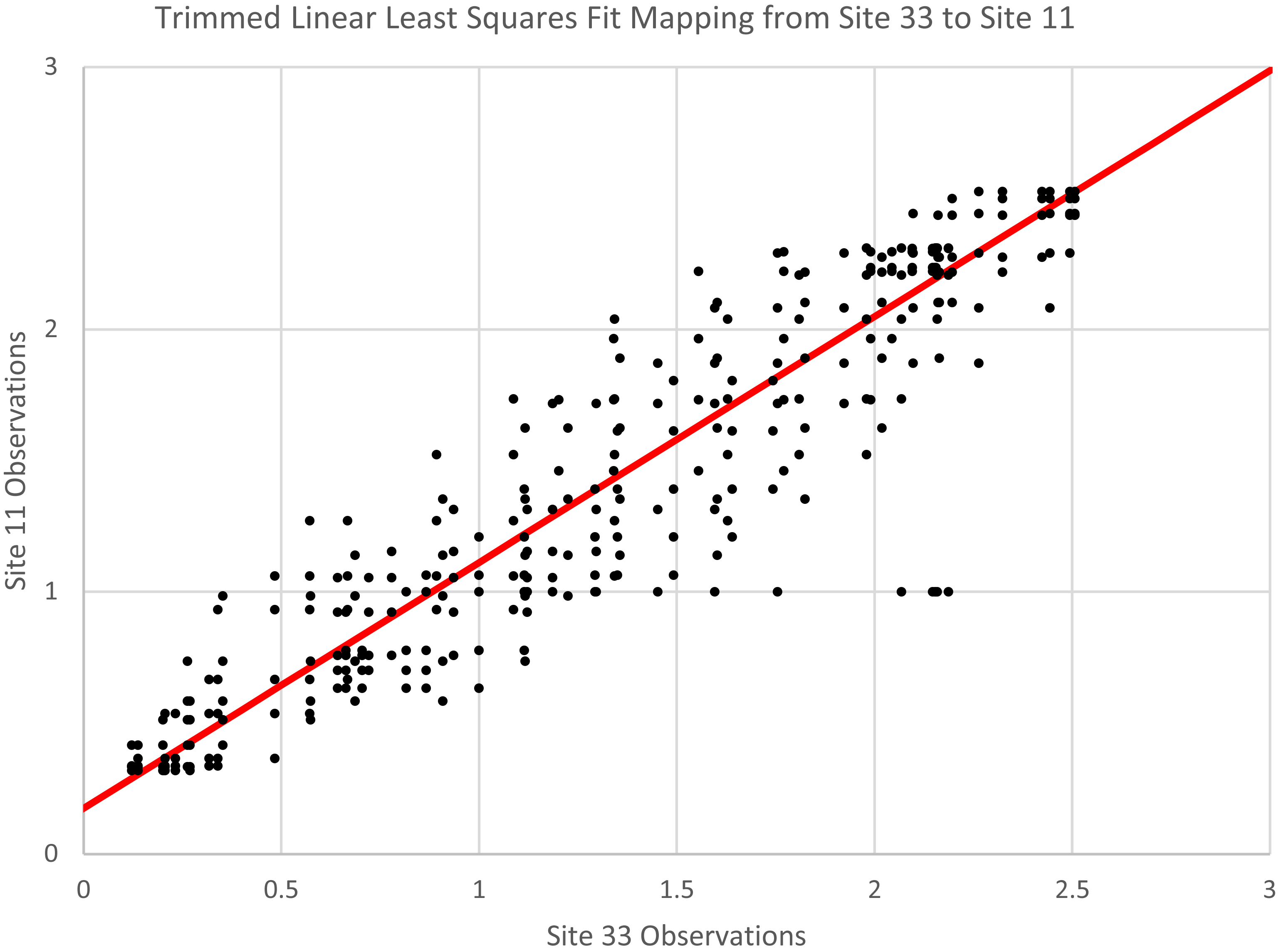

Before applying least trimmed squares to determine the linear fit, we select the percentage of data that will be trimmed before computing the fit. The trim percentage can be interpreted either as our willingness to accept bad data in our models or our estimation of how much data is bad. For our artificial data set we used a trim percentage of 0.1 since we defined several of our erroneous sites to have error rates near this value.

As an example, we show the linear mapping from Site 33 to Site 11 from our artificial data set using the paired observations from these sites within a time radius of 20. The inclusion of data with different time offsets will subsequently provide us with a simple and effective method to account for varying time offsets by way of the quadratic error function. We then apply least trimmed squares linear regression with a trim percentage of 0.1. See Fig. 3. Notice the pairs that include the erroneous observations from Site 11 where the value from that site is 1.0. These are apparent outliers and least trimmed squares helps to eliminate their influence on the result.

Least trimmed squares linear regression yields the following linear fit, mapping observations from Site 33 to Site 11: $l_{33,11}\left(x\right)=0.174376+0.937449x$ . We will refer to the coefficients as $l.a=0.174376$ and $l.b=0.937449$ . $l.\textit{mse}=0.03655$ is the mean-squared-error of the linear fit to the un-trimmed data from the final fit.

We now model the squared error of the linear fit relative to the time offset of the observations from the two sites using a quadratic model. Again, we use least trimmed squares to accomplish this. See Fig. 4. The least trimmed squares quadratic fit that maps time differences of observations from Site 33 and Site 11 to the squared error between the linear mapping from Site 33 and Site 11 and actual observations from Site 11 is: $q_{33,11}\left(\Delta t\right)=0.015933+0.00063\left(\Delta t\right)+0.000166% \left(\Delta t\right)^{2}$ . We refer to the coefficients as $q.a=0.015933$ , $q.b=0.00063$ , and $q.c=0.000166$ ; and $q.\textit{mse}=0.001608$ is the mean-squared error of the fit. Several additional values are derived: $q.\textit{axis}=1.890715$ and $q.\textit{extreme}=0.015339$ , which represent the axis of symmetry and the extreme value of the quadratic error expression respectively.

Figure 4.

Least trimmed squares quadratic fit mapping squared errors for linear mapping of observations from Site 33 to Site 11.

Despite our efforts to make the linear site-to-site mappings and quadratic estimates of error robust, there are cases in which the results will be unusable due to bad data or poorly aligned data resulting from large differences in reporting times and infrequent reporting. We can check the coefficients and derived measures for unexpected or unusable results.

3. The SMART estimator and accuracy assessment

In this section, we present our SMART estimator, first developed in [23], after looking at standard, interpolation-based aggregate estimators. Formally: Let $S$ be the set of all sites. Let $s\in S$ be a site for which we are evaluating observations. Let $\langle s_{1},\ldots,s_{n}|s_{i}\in S,s_{i}\neq s\rangle$ be the set of sites other than site $s$ . Then we wish to estimate ${\textit{obs}}_{s}\left(t_{s}\right)$ , the value of the observation at site $s$ at time $t_{s}$ using the most recent observations from the other sites relative to time $t$ : $\left(t_{i},v_{i}\right)$ .

3.1 Popular interpolators

Inverse Distance Weighting (IDW) [39] estimates are the weighted average of observation values, using (geographic) distance from the site/location for which an observation is to be estimated as the weight, raised to some exponent $h$ . If ground truth is known, a suitable exponent $h$ can be determined to minimize error in the estimate of ground truth. If $h=$ 0, then the estimate becomes a simple average of all observations. For large values of $h$ , the estimate tends to the nearest neighboring observation(s). For experiments with our artificial data set, we used $h=$ 0.8. This simple version of IDW does not account for time, so it is assumed that observations fall relatively close to each other in terms of time offset.

Least Squares Regression (LSR) maps the coordinates of the sites to the observed values. We only use $x-y$ coordinates in our experiments for LSR. There could be benefit in using elevation and other variables including time. However, doing so compounds problems related to bad metadata such as incorrect locations, bad timestamps and incorrect or inaccurate elevations.

Universal kriging (kriging with a trend) (UK) [40] uses the covariance between sites along with the coordinates of the sites and the observed values. In our experiments, we used a Gaussian covariance function of distance and estimated the related parameters so-as to minimize error relative to ground-truth for our training data. For kriging, the estimate of covariance could incorporate dimensions such as time and elevation as well, but finding a representative covariance function may be challenging. Alternatively, kriging could be used with covariances computed individually on pairs of sites rather than as a global function. Site-to-site covariance could implicitly account for elevation and other factors. This would be beneficial and would alleviate the challenges of determining an overall covariance function, but a robust approach would have to be used in doing this to mitigate the impact of bad data.

All of these methods can be applied using a restricted radius around the point at which the estimate is to be made or within a restricted bounding box or similar to alleviate computational challenges and to focus on local trends. Other interpolators could be applied in a similar manner. There are obvious risks in using these and other interpolators. Outliers and erroneous values will have an adverse impact on interpolation, causing poor estimates. Lack of data in proximity to a point to be estimated can also result in a poor estimate.

3.2 Our SMART interpolator

Our SMART interpolator is similar to IDW and uses our quadratic error estimate as the distance given the time lag between observations and our SMART linear mappings to yield estimated ground truth producing the estimate:

$\displaystyle\text{SMART}\_\text{estimate}_{s}\left(t_{s}\right)=\frac{\sum% \limits_{i=1}^{n}\left(\frac{1}{q_{s,s_{i}}\left({t}_{s}-{t}_{i}\right)}\right% )^{g}{l}_{s,s_{i}}\left(v_{i}\right)}{\sum\limits_{{i=1}}^{n}\left(\frac{1}{q_% {s,s_{i}}\left(t_{s}-t_{i}\right)}\right)^{g}}$ (5)

Neither distance nor direction are directly used in the computation. The linear mappings and quadratic error estimates account for similarity between sites. No attempt is made to down-weight clustered sites, although there may be benefit in doing so.

We determine the exponent by minimizing error relative to ground truth, if available. For the artificial data set, $g=$ 5.7 was determined. Prior to computing the weighted estimate, weights are examined and, if necessary, “re-balanced” in order to reduce the potential influence of single sites on the outcome. For instance, we found it useful to restrict the maximum relative weight a site can be given so-as to reduce the risk that a bad value from one site will over influence the resulting average.

Rather than take a simple weighted average, we use a trimmed mean to reduce the influence of outliers on the result. We employ Least Trimmed Squares as a metaheuristic and compute the mean relative to the weights while minimizing the (weighted) mean-squared-error relative to the non-trimmed data.

The algorithm for our SMART estimator is as follows. Note that the constants are specific to our artificial data set.

Algorithm 1. $\textit{SMART}{\_}\textit{ESTIMATE}$ ( $s$ , $S$ , $t$ )
Input: Let $S$ be the set or a subset of all sites. Let $s\in S$ be a site for which we are evaluating values/observations. Let $\langle s_{1},\ldots,s_{n}\|s_{i}\in S,s_{i}\neq s\rangle$ be the set of sites other than site $s$ . Let t be the time for which the prediction will be made.
Constants: $\textit{maxweight}=0.25\in(0,1]$ , $\textit{trimpct}=0.1\in(0,1]$ , $\textit{minvalidqfit}=0.0001\in(0,1]$ $\textit{maxvalidqfit}=0.5\in(0,1]$ , $\textit{iterations}_{\textit{max}}=100\in N$
Output: The estimate, predicted.
sumweights $=$ 0
weightedsum $=$ 0
for $i=$ 1 $\bm{to}$ $n$
if $\textit{VALID}\_\textit{MAPPING}\left(s_{i},s\right)$ then
let $\left(t_{s_{i}},v_{s_{i}}\right)=\textit{MOST}\_\textit{RECENT}\_\textit{OBS}% \left(s_{i},t\right)$
$x_{i}=l_{s_{i},s}(v_{s_{i}})$
$\Delta t=t-t_{s_{i}}$
$\textit{qfitval}=q_{s_{i},s}\left(\Delta t\right)$
if $(\textit{qfitval}>\textit{minvalidqfit})$ and $(\textit{qfitval}<\textit{maxvalidqfit})$ then
$\textit{weight}=\frac{1}{\textit{qfitval}}$
$w_{i}=\textit{weight}$
else
$w_{i}=0$
else
$w_{i}=$ 0
$x_{i}=$ 0
$\textit{NORMALIZE}\_\textit{WEIGHTS}\left(w\right)$
$\textit{BALANCE}\_\textit{WEIGHTS}\left(w,\textit{maxweight}\right)$
$\textit{predicted}=W\_\textit{TRIMMED}\_\textit{MEAN}\left(x,w,\textit{trimpct% },\textit{iterations}_{\textit{max}}\right)$
return predicted

$\textit{NORMALIZE}{\_}\textit{WEIGHTS}\left(w\right)$ normalizes weights to sum to 1. Weights must be non-negative.

$\textit{BALANCE}{\_}\textit{WEIGHTS}\left(w,\textit{maxweight}\right)$ reduces any weights that exceed the maximum specified and redistributes the excess weight proportionally to remaining elements. Iteration may be necessary in the event that a redistributed weight exceeds the maximum specified.

$W\_\textit{TRIMMED}{\_}\textit{MEAN}\left(x,w,\textit{trimpct},\textit{% iterations}_{\textit{max}}\right)$ uses the iterative least trimmed squares metaheuristic to determine the optimal mean in terms of mean squared error relative to the untrimmed data.

3.3 Experimental results: Artificial data

Using the data from the first time period/weather pattern in our artificial data set, we created mappings between all sites and then made estimates for other time periods. We compared results to those for IDW, LSR and UK. For LSR we investigated three cases with varying radii: a maximum of 50 units, a maximum of 100 units and no maximum/all data. For UK we used a radius of 150 which was chosen as a value for which computation time was still reasonable while not restricting too much data. The mean-squared-error (MSE) over all predictions versus ground truth shows that our SMART method dramatically out-performs the other methods. See Table 2.

Table 2
MSE from ground truth for interpolators

SMART	IDW	LSQR50	LSQR100	LSQRALL	UK150
0.088	1.110	11.8175	6.228	1.413	2.980

Figure 5.

Ground truth, observed and predicted values from the SMART method for Site 11 and errors.

To further demonstrate the performance of our SMART method, we examine Site 11 relative to errors over one of the evaluation weather patterns. See Fig. 5. During the evaluation time period there were three erroneous observations from Site 11. The SMART method predicted values that approximated ground truth reasonably well but with several notable exceptions: the first estimated low occurs subsequent to the actual low, there are jumps in the estimated value, and the second low is underestimated. The jumps are either a result of erroneous values from another site or from inclusion/exclusion of sites depending on reporting frequency and time offset. Still, the result is reasonable and could provide us with insight into how errors could be flagged. The two large errors stand out and would be identified without any false-positives using a cutoff in absolute error of 0.6 or greater. The third, smaller error is problematic. It would not be detected unless the cutoff was dropped below 0.5, which would result in a number of false positives because of the poor estimate of the second low.

As we demonstrate later, the example in Fig. 5 is relatively simple, and there are many types of problems that a site can exhibit. Given this example alone, one might ask why differences or derivatives computed on a series alone could not be used. The answer is that they could, and there certainly is room for derivatives to be incorporated into our method. However, derivatives alone will not identify all types of errors that we are interested in.

3.4 Experimental results: Real data from MADIS

We extracted real temperature observations from the MADIS Mesonet subset from December 2015 and bounded between 38.5 ${}^{\circ}$ N and 42.5 ${}^{\circ}$ N latitude and $-$ 124.5 ${}^{\circ}$ W and $-$ 119.5 ${}^{\circ}$ W longitude, covering California north of Sacramento and overlapping a portion of Oregon, Nevada and the Pacific Ocean. We used the first week in December for a training set and the second week for testing. All total, 890 sites had observations in this subset. Note that the weather was variable during this month. California finally received bad weather during the bad weather season in 2015 after several years of little or no winter. No artificial errors were introduced into the data – the data is used as-is.

Table 3
MSE by MADIS QCD for interpolators

QCD	SMART		IDW		LSQ50		LSQ100		LSQALL
Q	37.	64	397.	24	378.	36	358.	46	337.	20
S	7.	16	107.	26	79.	92	66.	84	60.	67
V	4.	16	125.	40	93.	11	74.	64	61.	06
X	85525.	63	95891.	65	96555.	19	96803.	05	97299.	10
ALL	97.	41	254.	49	225.	33	209.	36	199.	24

V $=$ verified/good, S $=$ subjective/good, X $=$ bad, Q $=$ questionable.

Figure 6.

Predictions for GISC1 from the interpolators.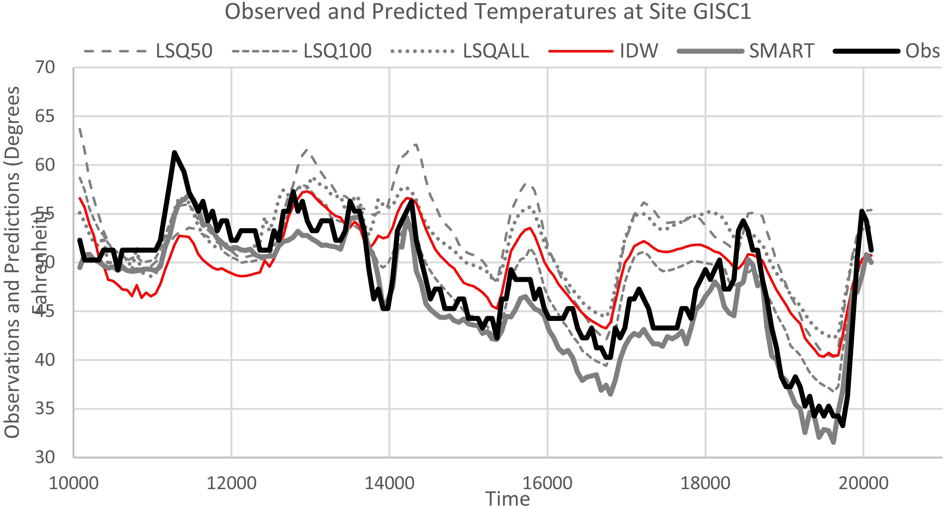

We compared our SMART method to IDW, LSQ50 (50 mile radius), LSQ100 (100 mile radius), and LSQALL (include all data). For all methods, the most recent observations from individual sites were used. We were not able to determine a consistent covariance model and could not get Universal Kriging to work with the MADIS data. Further issues were experienced with non-invertible matrices because of coincident sites, etc. Too much preprocessing would have been necessary, so we did not make predictions using Universal Kriging on the MADIS data set.

Since we do not have ground truth for this data set, we computed mean-squared error relative to observed value and grouped by quality control descriptors (QCD) provided by MADIS. The resulting mean-squared-error by method and QCD is shown in Table 3. The MSE results in Table 3 are very good.

Now we look at the results for site GISC1 (Gibson near Castella), which MADIS located in downtown Sacramento. For this site, our SMART method estimates were reasonably close to the observed values whereas all of the other methods tended to overestimate. See Fig. 6. The MADIS QCD indicators showed a great deal of uncertainty regarding the observations from this site with a mix of Q (questionable), S (subjective) and V (verified) values. However, when we compared the corresponding observations to the absolute error of predictions from our SMART method, there was no apparent pattern. See Fig. 7. There is no apparent pattern in the absolute errors from the other methods either, although the absolute errors are greater relative to our SMART method.

Table 4

MSE by QCD for GISC1

	SMART	IDW	LSQ50	LSQ100	LSQALL
Q	6.613	34.528	90.706	19.340	62.990
S	5.202	22.287	26.250	7.112	25.041
V	8.808	9.733	23.103	4.959	18.688
ALL	6.839	20.570	40.070	9.169	31.544

QCD counts: Q $=$ 39, S $=$ 68, V $=$ 61, Total $=$ 168.

Figure 7.

Observations (by QCD) and predictions for site GISC1 (gibson near castella).

Our SMART method performs better overall but worse than LSQ100 for the V data for Site GISC1. See Table 4. And, it performs better for the Q and S data than for the V data, particularly for the Q data. One way this could happen would be if the data was mislabeled. In fact, we are confident that it is mislabeled because we know that this site was mis-located by MADIS and, as a result, the MADIS level 3 check is invalid. This site is not located in downtown Sacramento but is located 170 miles to the north of Sacramento. The reason it fails MADIS level 3 quality control resulting in Q values for QCD is that quite often it does not agree with sites located in downtown Sacramento. There are times when it comes close, and those times correspond to S and V QCD indicators, but many times the differences are large enough that MADIS flags observations from this site as failing.

Our SMART method helps to identify further site-related problems such as incorrect locations. Next we identify site-related problems including bad metadata.

4. Bad sites and bad metadata

In this section, we show informally how our SMART mappings can be analyzed to identify bad sites and bad metadata. We compare the coefficients and derived measures from the SMART mappings and look for outliers in those values. We use the general term “bad site” to refer to a site that produces erroneous data. As mentioned earlier, it is not our intent at this point to diagnose specific problems. There are many types of erroneous metadata including incorrect or misspelled site names, mismatched sensor type, wrong units, etc. We focus our attention here on two types of bad metadata: incorrect location and bad timestamps. Both of these error types will adversely affect the interpolation methods that make use of this information, and the effect can be dramatic.

4.1 Identification of bad sites

We first looked at the coefficients and MSE values for the site-to-site mappings and determined how these could be used to identify “bad” sites. Initially, for our artificial data set, we labeled sites as “bad” if they included erroneous data. Of course, there are varying degrees of bad. In general, for data sets in which we do not have ground truth, we will not know which sites are bad a priori. In fact, all sites may be bad to one degree or another simply due to lack of precision or accuracy. We found that sites with large numbers of outlying $l . a$ , $l . b$ and $l.\textit{mse}$ values corresponded to bad sites. Not surprisingly, sites with fewer errors and sites with smaller-scaled errors did not produce outlying values because of the robust methods employed in determining their SMART mappings.

We again used the temperature observations from the MADIS Mesonet subset, as described earlier.

4.1.1 Sites for which mappings could note be determined

There were 36 MADIS sites for which site-to-site mappings could not be determined during the training period. We examined these sites individually and the results are not surprising, with each site exhibiting one or more of the following issues: there was little or no data during the training period, there were large gaps in reporting, or there was a very narrow range in reported data. These sites could have readily been identified by filtering sites based on measures such as temporal completeness [1, 2]. Still, their handling is non-trivial. Some of these sites began reporting data during the testing period and some of that data could have been useful depending on the application. A potential disadvantage of using our SMART mappings is that we will disregard such sites until a new training period has passed in which there is sufficient data to produce mappings for them. One could argue that it is prudent to hold out data from such a site until the site can be proven to produce quality data.

Figure 8.

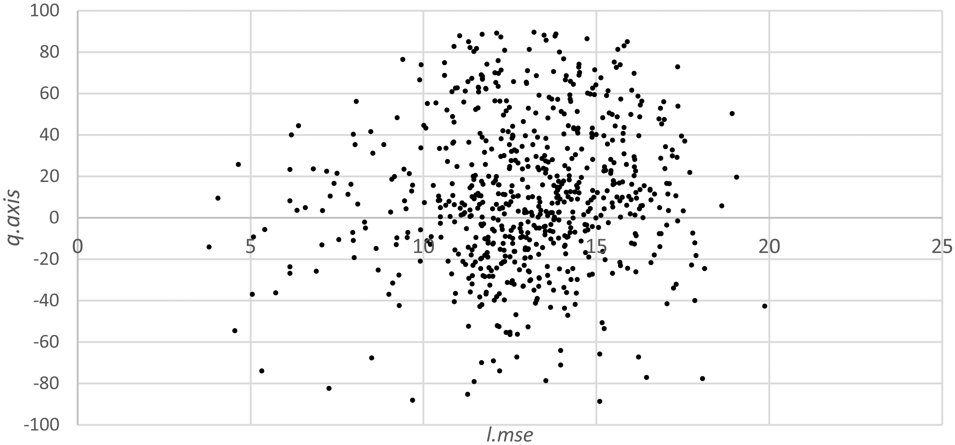
Sorted $l . a$ values for sites from MADIS subset.

Figure 9.

Sorted $l . b$ values for sites from MADIS subset.

4.1.2 Bad sites determined by SMART site-to-site mappings

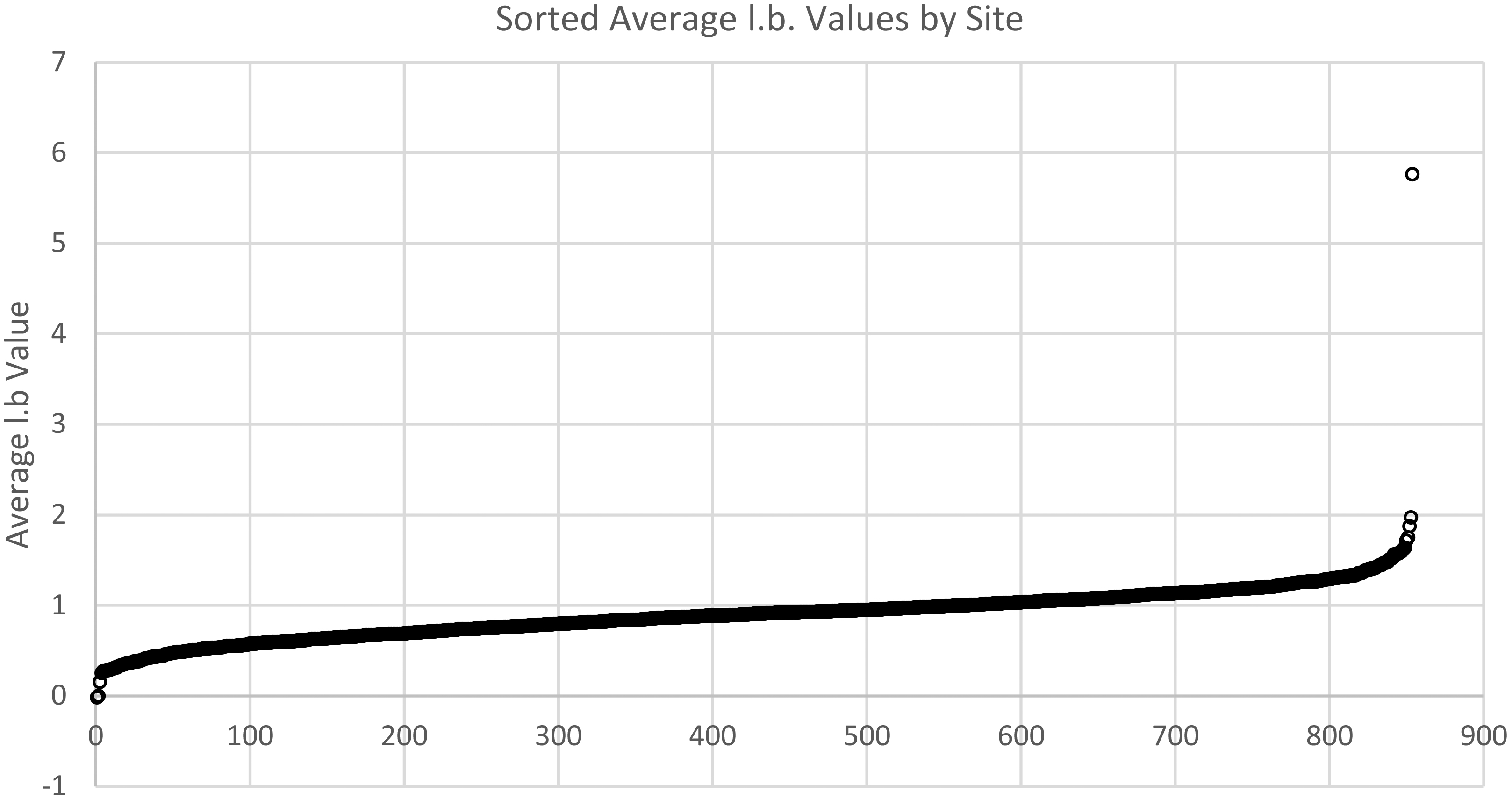
For each site, we averaged the $l . a$ values for all mappings to that site. Even though there were outliers in the individual $l . a$ values, we used the arithmetic mean for the average. A more robust measure such as trimmed mean or median could be used to mitigate the impact of outliers if necessary. For those sites having an average $l . a$ value on the extreme negative side, the corresponding site has observations far lower than most other sites. For those having an average $l . a$ value on the extreme positive side, the corresponding site has observations far higher than most other sites. At first, we may consider such sites questionable and should seek a reasonable explanation for their behavior. It is possible that a high mountaintop site will experience lower temperatures than all or most other sites. And, it is possible that a low desert site will experience higher temperatures than most other sites. But if the differences are extreme, particularly in comparison to other similarly-located sites, then such a site should be considered “bad”/erroneous, and it should be held out from further analysis until the associated problems are rectified. From observation of the apparent outliers we set our cutoff for $l . a$ as ( $-$ 56.73, 51.33), with any site having an average $l . a$ value outside this interval labeled “bad”. See Fig. 8.

For the average $l . b$ coefficients we found a cutoff interval of (0.16, 1.71). See Fig. 9. For this dataset, we do not expect negative $l . b$ values since there should be a positive correlation between sites, at least nearby sites for which clocks are synchronized. We do not expect $l . b$ values of zero since that would signify that a site has non-changing observations. And, we do not expect large values for $l . b$ since the would signify ranges for a site outside the norm of that for other sites. For the average $l.\textit{mse}$ values by sites, the outliers mostly overlapped with the outliers for the $l . a$ and $l . b$ values. We did find several sites that had an outlier $l.\textit{mse}$ value despite not having outlier $l . a$ or $l . b$ values, so it was worthwhile to check these as well, and a cutoff interval of (1.58, 31.82) was used for $l.\textit{mse}$ .

Figure 10.

Site 293 from MADIS subset showing sporadic reporting and extreme negative temperatures.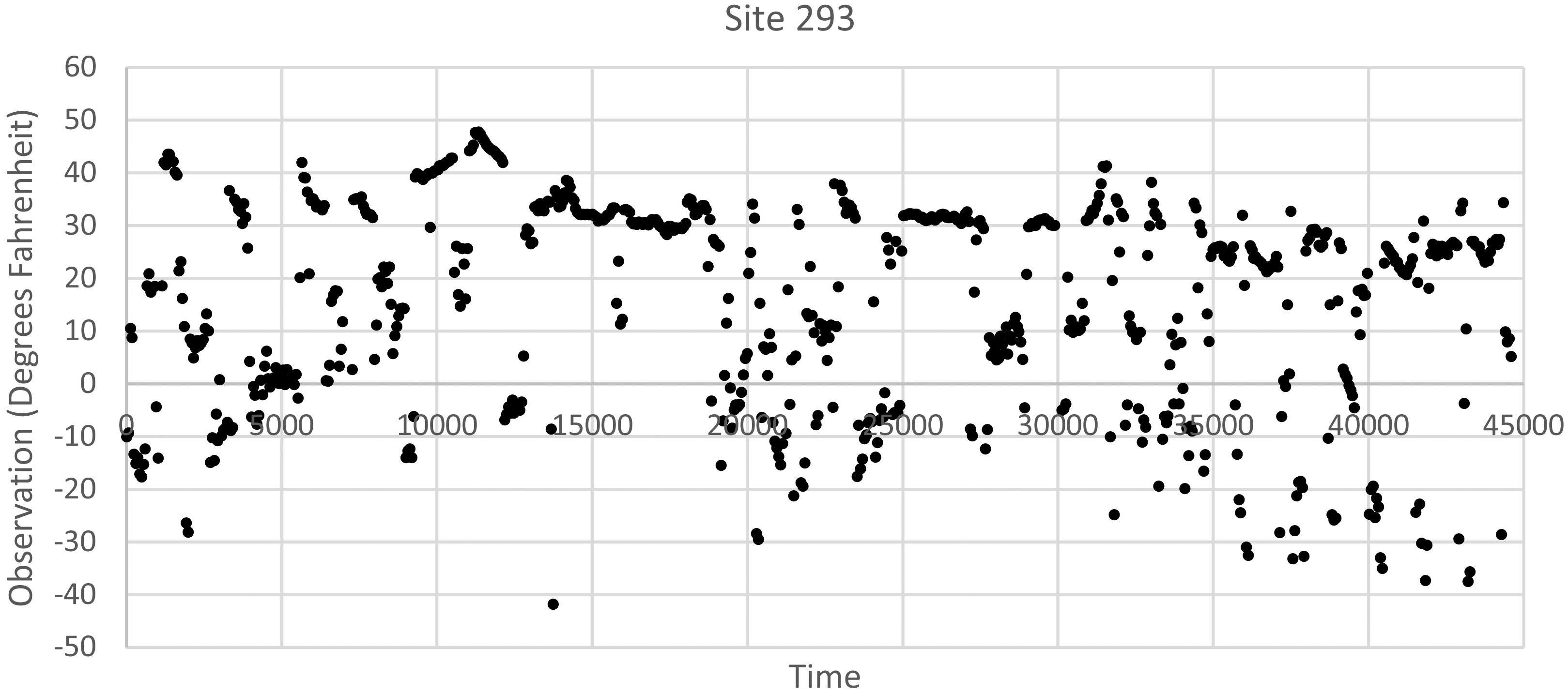

After determining the prospective outlier sites using the site averages of the $l . a$ , $l . b$ and $l.\textit{mse}$ values, we then examined each prospective outlier site. In every case, there was at least one of the following logical explanations as to why the site was an outlier: multiple apparent series rather than one, constant or near constant values, many outliers, large outliers, range of values much wider than the normal range, wild variation, gaps or sparse data during training period, sporadic reporting, or generally doesn’t follow the expected trend. Figure 10 shows one example “bad site” with extreme negative values and sporadic reporting.

4.2 Bad location metadata

In order to develop an approach for identifying bad location metadata, we again needed a representative ground truth dataset. For this purpose, we used the Mesoscale Analysis and Prediction System (MAPS) and the Rapid Update Cycle (RUC) Surface Assimilation Systems (MSAS/RSAS) dataset from NOAA for air temperatures in the Northern California area for the entire month of December 2015 [41, 42]. The MSAS/RSAS data provides estimated surface observations for grid points with 8-mile spatial and one-hour temporal resolution. Since 1-hour temporal resolution was not sufficient for our analysis and was not representative of frequency of reporting of site-based sensor observations, we used bicubic splines to interpolate down to 1-minute temporal resolution. We used existing MSAS/RSAS grid points as site locations, and did not attempt further spatial interpolation to construct site-based observations.

In general, the series from near sites should be similar and the series from far sites should be less similar. The $l.\textit{mse}$ values from our SMART mappings give an indication of similarity, and we expected a positive correlation between $l.\textit{mse}$ and the (geographic) distance between sites, with the lowest $l.\textit{mse}$ values corresponding to the nearest sites. We found this relationship to hold for various points selected from the RSAS grids. To investigate mis-located sites, we relocated grid points (changed their location metadata) and found, as expected, that the near points no longer had the least $l.\textit{mse}$ values. Points corresponding to the changed locations showed the least $l.\textit{mse}$ values, indicating that the site was mis-located. Mis-location by lesser distances show similar behavior and can be identified as well.

We now turn our attention to sites in the MADIS set. For this experiment, we used data for the entire month of December 2015. We found a number of mis-located sites using the relationship between distance and $l.\textit{mse}$ .

For instance, MADIS mis-located Site WVVCA at (40.680, $-$ 120.83), near Eagle Lake 105 miles to the east of its correct location. See Fig. 11 and note that sites having the lowest $l.\textit{mse}$ values fall approximately 100 to 110 miles from the sites reported location. MADIS subsequently relocated this site to (40.680, $-$ 122.830) along State Route 299 and near Weaverville. The WVV likely stands for Weaverville. Notice that the incorrect longitude was $-$ 120.83 and the correct longitude was $-$ 122.830. There was likely a transcription error for this site. The plot of distance versus $l.\textit{mse}$ identifies this site as being mis-located, and shows that it is mis-located by approximately 105 miles, matching the correction that was subsequently made by MADIS.

Figure 11.

Distance versus $l.\textit{mse}$ for site-to-site comparison of WVVCA site from the MADIS subset with other MADIS sites. This site was mislocated near Eagle Lake 105 miles to the east of its correct location near Weaverville by MADIS.

MADIS mis-located Site KLHM (Lincoln Regional Airport) at (38.91, $-$ 120.65), 37.6 miles to the east of its correct location, and subsequently relocated it to the Lincoln Regional Airport at (38.910, $-$ 121.350). Given that the latitudes correspond and the longitudes differ, transcription error is again suspected.

As mentioned earlier, Site GISC1 (Gibson near Castella) was mis-located by MADIS at (38.56556, $-$ 121.485) in downtown Sacramento. Weathershare users identified this site as mis-located. The incorrect location data persisted for years in the MADIS feed but was finally updated some time in 2016, separate from and subsequent to our analysis. It was corrected by MADIS to (41.022, $-$ 122.399), 175 miles to the north near the Caltrans Gibson Maintenance yard and near the town of Castella. For the December 2015 data, the mis-location of GISC1 was readily apparent in the plot of distance versus $l.\textit{mse}$ . It may have previously been assigned the coordinates of another site.

Our approach for identifying mis-located sites does work, as confirmed by examination of sites known to have been mis-located by MADIS. While the approach we have outlined identifies large errors, it should be possible to identify lesser errors. Our method also shows promise in identifying the approximate correct location for a mis-located site by way of the location of the sites corresponding to the least $l.\textit{mse}$ values. It is important to identify these in a grouped, robust fashion rather than simply use the site with the least $l.\textit{mse}$ value since that site too may be mis-located.

4.3 Bad timestamps

The last type of error we investigate is bad timestamps. It is our belief that many if not most of the MADIS sites have data for which the timestamps are not synchronized with the correct time. In order to investigate this possibility, we started again with the RSAS data. Here we made an assumption that clocks were synchronized and timestamps were correct for sites represented by grid points in the RSAS data. We then plotted $l.\textit{mse}$ versus $q.\textit{axis}$ and investigated the data relative to the line $q.\textit{axis}=$ 0. We used $l.\textit{mse}$ rather than distance because of problems with mis-location of sites as demonstrated in the previous section and with the intent of being able to better discern similar sites. For low $l.\textit{mse}$ values, $q.\textit{axis}$ values should be near zero. Generally the $q.\textit{axis}$ values should be centered around $q.\textit{axis}=$ 0. This pattern held for the RSAS data. When we shifted timestamps for a site/grid point by a fixed amount $s$ , we saw a similar pattern, but the plot was shifted and now fell so that the $l.\textit{mse}$ values were approximately centered around $q.\textit{axis}=s$ , matching the shift $s$ in the timestamps. Thus, sites for which a shift is apparent likely have bad timestamps.

We next investigated the MADIS data to see if we could find similar patterns to identify sites with bad timestamps. Unlike the mis-located sites for which we could be certain of the original errors and subsequent corrections for several sites, we do not have concrete examples for which we know that the timestamps are incorrect. However, we are fairly certain that the extreme errors we identify correspond to real errors in the timestamps.

We believe that the timestamps for the Caltrans Dunsmuir (CTDUN) site are correct or nearly correct. The plot of $l.\textit{mse}$ versus $q.\textit{axis}$ for CTDUN appears to confirm this, with $q.\textit{axis}$ values centered approximately at $q.\textit{axis}=$ 0. See Fig. 12. We see greater variability in the data than we saw for the RSAS data. This is attributable to greater variability in the underlying data, differences in reporting intervals, and (we hypothesize) offsets (non-synchronization) of the clocks. With this said, we believe that the timestamps are correct or at least very nearly correct for CTDUN. The general appearance is that the dataset appears is split evenly by $q.\textit{axis}=$ 0.

Figure 12.

$l.\textit{mse}$ versus $q.\textit{axis}$ for site-to-site comparison of caltrans dunsmuir site from the MADIS subset with other MADIS sites.

Figure 13.

$l.\textit{mse}$ versus $q.\textit{axis}$ for site-to-site comparison of BUGC1 from the MADIS subset with other MADIS sites.

Site BUGC1, is located in a remote part of the Klamath National Forest near near Bestville, approximately 47.5 miles west of Dunsmuir. When we plot $l.\textit{mse}$ versus $q.\textit{axis}$ for site mappings to BUGC1, we see that they are centered at a $q.\textit{axis}$ value of $-$ 50 or less, so we believe the time offset for timestamps from this site is large. See Fig. 13.

We found numerous other examples of sites for which we are confident that the timestamps are incorrect, and we have found a great deal of variability in this data. Ultimately, we believe that there are both large and small errors in the timestamps.

5. Conclusions

The SMART method presented in this paper shows promise as an interpolator for spatio-temporal data in the presence of errors. It accounts for errors in multiple facets of the interpolation process. In terms of neighborhood formation, it maps like sites to like sites rather than assignment based on geographic proximity, and it assigns weights according to quadratic error in simple, linear mappings. Through the use of least trimmed squares, errors are mitigated up to a predetermined tolerance level. In turn, a trimmed, weighted mean is used to compute final, interpolated values, reducing the potential for single or even multiple erroneous values to bias the result. In tests with a representative, artificial data set, we demonstrate that this approach far out-performs popular interpolation methods in estimating ground truth in the presence of multiple types of errors. It also outperforms these methods in ability to distinguish bad data from good data. With a real data set we find similar results in terms of estimation, although we are challenged by not having ground truth, and use provider quality control flags to perform evaluation. When investigating ability to distinguish bad data from good data we find that the provider quality control flags are questionable. We further demonstrate that bad metadata such as incorrect location data can adversely affect results.

We presented a representative method for accuracy assessment and compared and contrasted it with other interpolation methods to demonstrate the importance of mitigating erroneous data throughout the process. All interpolation methods presented are susceptible to erroneous data, particularly if used as-is. Their use must account for and mitigate erroneous data. For instance, it is not sufficient to use robust estimates of covariance to get good results with kriging methods. Kriging methods will still fail in the presence of erroneous data.

The SMART method presented in this paper also shows promise for identifying sites that have bad data. The simple (linear) site-to-site mappings and (quadratic) error estimates for the mappings can be used to identify erroneous sites. The coefficients of the mappings and associated performance measures can be compared across all sites, and outlier values of these parameters correspond to bad sites.

The SMART method further helps to identify bad location metadata and bad timestamp (unsynchronized) metadata. Using a raster dataset derived from meteorological sensor data as ground-truth, we developed and demonstrated methods to identify both of these types of bad metadata. In turn, we demonstrated that these methods identify known or highly likely instances of bad metadata in our original, site-based sensor data set.

Our SMART approach provides a representative method for assessing and handling site-based spatio-temporal data quality. In addition to providing assessment of accuracy at the observation level, our method helps to identify problematic sites including sites with bad metadata.

In future work, we intend to characterize the impact of the various components of spatio-temporal data quality including accuracy, precision, timeliness, reliability, completeness and coverage on interpolation-based methods for data quality assessment including our SMART method. We also intend to continue formalizing our method and test it against other datasets.

Footnotes

Acknowledgments

We acknowledge the California Department of Transportation (Caltrans) for its sponsorship of the WeatherShare project and other related projects. In particular, we acknowledge ian Turnbull and Sean Campbell from Caltrans. We further acknowledge Daniell Richter and other staff at the Western Transportation Institute for their work on WeatherShare, the Western States One Stop Shop and other related projects. The work presented in this paper has been conducted subsequent to and separate from this prior work.

References

Galarus

D.E.

and Angryk

R.A.

, Quality Control from the Perspective of the Real-Time Spatial-Temporal Data Aggregator and (re)Distributor, in ACM SIGSPATIAL ’14, 2014.

Galarus

D.E.

and Angryk

R.A.

, Spatio-temporal quality control: implications and applications for data consumers and aggregators, Open Geospatial Data, Softw. Stand. 1(1) (2016), 1.

Wang

R.Y.

and Strong

D.M.

, Beyond accuracy: What data quality means to data consumers, J. Manag. Inf. Syst. 12(4) (1996), 5–33.

Hunter

G.J.

Bregt

A.K.

Heuvelink

G.B.M.

De Bruin

and Virrantaus

, Spatial data quality: problems and prospects, in Research Trends in Geographic Information Science, Springer, 2009, 101–121.

De Veaux

R.D.

and Hand

D.J.

, How to Lie with Bad Data, Stat. Sci. 20(3) (2005), 231–238.

Richter

Wang

and Galarus

, WeatherShare Phase 2 Final Report, Mont. State Univ., 2009.

WTI/MSU, The Western States One-Stop-Shop for Rural Traveler Information [Online]. Available: http://oss.weathershare.org/ [Accessed: 29-Dec-2015].

NOAA, Meteorological Assimilation Data Ingest System (MADIS) [Online]. Available: http://madis.noaa.gov/ [Accessed: 26-Dec-2015].

U. of Utah, MesoWest Data [Online]. Available: http://mesowest.utah.edu/ [Accessed: 26-Dec-2015].

10.

Barnes

S.L.

, A technique for maximizing details in numerical weather map analysis, J. Appl. Meteorol. 3(4) (1964), 396–409.

11.

Shafer

M.A.

Fiebrich

C.A.

Arndt

D.S.

Fredrickson

S.E.

and Hughes

T.W.

, Quality assurance procedures in the Oklahoma Mesonetwork, J. Atmos. Ocean. Technol. 17(4) (2000), 474–494.

12.

Limber

Drobot

and Fowler

, Clarus Quality Checking Algorithm Documentation Report, techreport, 2010.

13.

Splitt

, Michael E; Horel, Use of Multivariate Linear Regression for Meteorological Data Analysis and Quality Assessment in Complex Terrain [Online]. Available: http://mesowest.utah.edu/html/help/regress.html [Accessed: 26-Dec-2015].

14.

U. of Utah, MesoWest Quality Control Flags Help Page [Online]. Available: http://mesowest.utah.edu/html/help/key.html [Accessed: 26-Dec-2015].

15.

NOAA, MADIS Quality Control. [Online]. Available: http://madis.noaa.gov/madis_qc.html. [Accessed: 26-Dec-2015].

16.

NOAA, MADIS Meteorological Surface Quality Control [Online]. Available: https://madis.ncep.noaa.gov/madis_sfc_qc.shtml [Accessed: 26-Dec-2015].

17.

Belousov

S.L.

Gandin

L.S.

and Mashkovich

S.A.

, Computer Processing of Current Meteorological Data, Translated from Russian to English by Atmospheric Environment Service, Nurklik, Meteorol. Transl. (18) (1972), 227.

18.

Zimmerman

Pavlik

Ruggles

and Armstrong

M.P.

, An experimental comparison of ordinary and universal kriging and inverse distance weighting, Math. Geol. 31(4) (1999), 375–390.

19.

G.Y.

and Wong

D.W.

, An adaptive inverse-distance weighting spatial interpolation technique, Comput. Geosci. 34(9) (2008), 1044–1055.

20.

Mueller

T.G.

Pusuluri

N.B.

Mathias

K.K.

Cornelius

P.L.

Barnhisel

R.I.

and Shearer

S.A.

, Map Quality for Ordinary Kriging and Inverse Distance Weighted Interpolation, Soil Sci. Soc. Am. J. 68(6) (2004), 2042.

21.

Galarus

D.E.

Angryk

R.A.

and Sheppard

J.W.

, Automated Weather Sensor Quality Control., in: FLAIRS Conf., 2012, pp. 388–393.

22.

Galarus

D.E.

and Angryk

R.A.

, Mining robust neighborhoods for quality control of sensor data, Proc. 4th ACM SIGSPATIAL Int. Work. GeoStreaming – IWGS ’13, Nov. 2013, 86–95.

23.

Galarus

D.E.

and Angryk

R.A.

, A SMART Approach to Quality Assessment of Site-Based Spatio-Temporal Data, in ACM SIGSPATIAL ’16, 2016.

24.

Galarus

D.E.

and Angryk

R.A.

, The SMART Approach to Comprehensive Quality Assessment of Site-Based Spatial-Temporal Data, in: 1st IEEE International Workshop on Big Spatial Data in Conjunction with the 2016 IEEE International Conference on Big Data.

25.

Tomczak

, Spatial Interpolation and its Uncertainty Using Automated Anisotropic Inverse Distance Weighting (IDW) – Cross-Validation/Jackknife Approach, J. Geogr. Inf. Decis. Analy. 2(2) (1998), 18–30.

26.

Joseph

V.R.

and Kang

, Regression-based inverse distance weighting with applications to computer experiments, Technometrics 53(3) (2011), 254–265.

27.

Stahl

Moore

R.D.

Floyer

J.A.

Asplin

M.G.

and McKendry

I.G.

, Comparison of approaches for spatial interpolation of daily air temperature in a large region with complex topography and highly variable station density, Agric. For. Meteorol. 139(3–4) (2006), 224–236.

28.

Ishida

and Kawashima

, Use of cokriging to estimate surface air temperature from elevation, Theor. Appl. Climatol. 47(3) (1993), 147–157.

29.

Vicente Serrano

S.M.

Sánchez

and Cuadrat

J.M.

, Comparative analysis of interpolation methods in the middle Ebro Valley (Spain): application to annual precipitation and temperature, 2003.

30.

Hubert

Rousseeuw

P.J.

and Segaert

, Multivariate functional outlier detection, Stat. Methods Appl. 24(2) (2015), 177–202.

31.

Hubert

Rousseeuw

Segaert

and others, Rejoinder to ‘multivariate functional outlier detection’, Stat. Methods Appl. 24(2) (2015), 269–277.

32.

Hubert

Raymaekers

Rousseeuw

P.J.

and Segaert

, Finding Outliers in Surface Data and Video, arXiv Prepr. arXiv1601.08133, 2016.

33.

Rousseeuw

P.J.

and Van Driessen

, Computing LTS regression for large data sets, Data Min. Knowl. Discov. 12(1) (2006), 29–45.

34.

Shekhar

C.T.

and Zhang

, A unified approach to detecting spatial outliers, Geoinformatica 7(2) (2003), 139–166.

35.

U. of Utah, MesoWest Quality Control Information Help Page [Online]. Available: http://mesowest.utah.edu/html/help/qc.html [Accessed: 01-Jan-2001].

36.

Voss

R.F.

, Random fractal forgeries, in Fundamental algorithms for computer graphics, Springer, 1985, 805–835.

37.

Feder

, Fractals. Springer Science & Business Media, 2013.

38.

Barnsley

M.F.

et al., The science of fractal images. Springer Publishing Company, Incorporated, 2011.

39.

Shepard

, A two-dimensional interpolation function for irregularly-spaced data, in: 23rd ACM Natl. Conf., 1968, pp. 517–524.

40.

Huijbregts

and Matheron

, Universal kriging (an optimal method for estimating and contouring in trend surface analysis), in: Proceedings of Ninth International Symposium on Techniques for Decision-making in the Mineral Industry, 1971.

41.

NOAA, MSAS/RSAS, 2013 [Online]. Available: http://msas.noaa.gov/ [Accessed: 24-Sep-2016].

42.

NOAA, The MSAS/RSAS Surface Analysis, 2007 [Online]. Available: http://msas.noaa.gov/msas_descrip.html.

Beyond accuracy – A SMART approach to site-based spatio-temporal data quality assessment

Abstract

Keywords

1. Introduction

1.2 Literature review

2. Smart mappings

2.1 Artificial dataset

Table 1 Errors introduced into sites from artificial dataset

3.1 Popular interpolators

3.2 Our SMART interpolator

Table 2 MSE from ground truth for interpolators

Table 3 MSE by MADIS QCD for interpolators

4.1 Identification of bad sites

4.1.1 Sites for which mappings could note be determined

Footnotes

Acknowledgments

References

Table 1
Errors introduced into sites from artificial dataset

Table 2
MSE from ground truth for interpolators

Table 3
MSE by MADIS QCD for interpolators