Forecasting,clustering and patrolling criminal activities

Abstract

Tools that perform pattern recognition analysis of crimes, comprising at the same time forecasting, clustering, and recommendations on real data such as patrolling routes, are not fully integrated; modules are developed separately, and thus, a single workflow providing all the steps necessary to perform this analysis has not been reported. In this paper, we propose forecasting criminal activity in a particular region by using supervised classification; then, to use this information to automatically cluster and find important hot spots; and finally, to optimize patrolling routes for personnel working in public security. The proposed forecasting model (CR- $\Omega+$ ) is based on the family of Kora- $\Omega$ Logical-Combinatorial algorithms operating on large data volumes from several heterogeneous sources using an inductive learning process. We perform two analyses: punctual prediction and tendency analysis, which show that it is possible to punctually predict one out of four crimes to be perpetrated (crime family, in a specific space and time), and two out of three times the place of crime, despite of the noise of the dataset. The forecasted crimes are then clustered using a density-based clustering algorithm, and finally route patrolling routes were crafted using an ant-colony optimization algorithm. For three different patrolling requirements, we were always able to find optimal routes in shorter time compared to commonly used random walk algorithms. We present a case study based on real crime data from the municipality of Cuautitlán Izcalli, in Mexico.

Keywords

Forecasting models for crime analysis public security patrolling routes optimization ant-colony systems Spatio-temporal similarity function pattern recognition supervised classification clustering

1. Introduction

Public security and crime fighting are one of the most important social priorities in great cities of the world. Despite the surprisingly big quantity of human and material resources that governments assign for this matter, it is still evident the need for alternative mechanisms that allow to increase the effectiveness and efficiency of police forces [12]. One of the main variables that limit this effectiveness is the response time to crime events. Particularly, immediate-reaction events show that the marginal improvements obtained in this matter are not enough to reduce the general criminal incidence of the zone, as well as to substantially modify the perception of insecurity between citizens [19].

A better perspective of this situation can be achieved if the problem is translated to the sphere of prevention instead of reaction. If public forces were capable to anticipate when and where the criminal activity of a specific kind might be increased, a double benefit could be achieved. On one hand, it would be possible to concentrate resources and logistic activity necessary to fight that specific kind of criminal activity in the anticipated place and time. On the other hand, it could be possible to establish dynamically and with solid foundations several of the common parameters of everyday work in public security, such as the specific design of surveillance rounds, the distribution of forces in time and space, and, of course, the development of security operations, or even information and prevention campaigns through massive communication media [28].

Several systems have been already created in order to help crime analysts in their duties, for example STAC (Spatial and Temporal Analysis of Crime) [w1], and CrimeLink (PCI Precision Computing Intelligence) [w2]. This latter system provides an Event-Time graph, and a Pattern Analysis wheel. Other systems are CrimeView (Omega Group) [w3], and ArcGis (Crime Analysis Extension), providing hotspot analysis on ArcGIS 9, main centroid identification, and probable crime direction identification. More recently, A.T.A.C (Automated Tactical Analysis of Crime) [w4] identifies criminal patterns through data ordering; it provides tools for analysis such as time series based prediction, Google Earth integration, mapping and density analysis. These systems are of great help in crime analysis and prevention; however, being mostly built for commercial purposes, they do not disclose their forecasting algorithms, making difficult to adapt them to the needs of a certain region. Moreover, these systems are not designed to provide recommendations, such as patrolling routes modeling, that are able to guarantee an adequate coverage of the identified hotspots.

In view of this, our work is devoted to a two-folded objective: first, we aim to study the spatial and temporal decisions made by criminals identifying hotspots where criminal activity is concentrated; while the second one is, once these activities are found and properly clustered, to provide a flexible schema – adapted to real needs and availability of resources – for designing adequate patrolling routes that optimally cover these hotspots.

In the following section (Section 2) we will focus on the forecasting of criminal activities; in Section 3 we tackle the problem of clustering and GIS-mapping these activities for the analyst. In Section 4 we cover the problem of patrolling routes design. In Section 5 we present a set of experiments and results of each one of the modules comprising this framework; and finally, in Section 6 we draw our conclusions.

Figure 1.

General architecture of the computerized system to support decision-making processes in public security.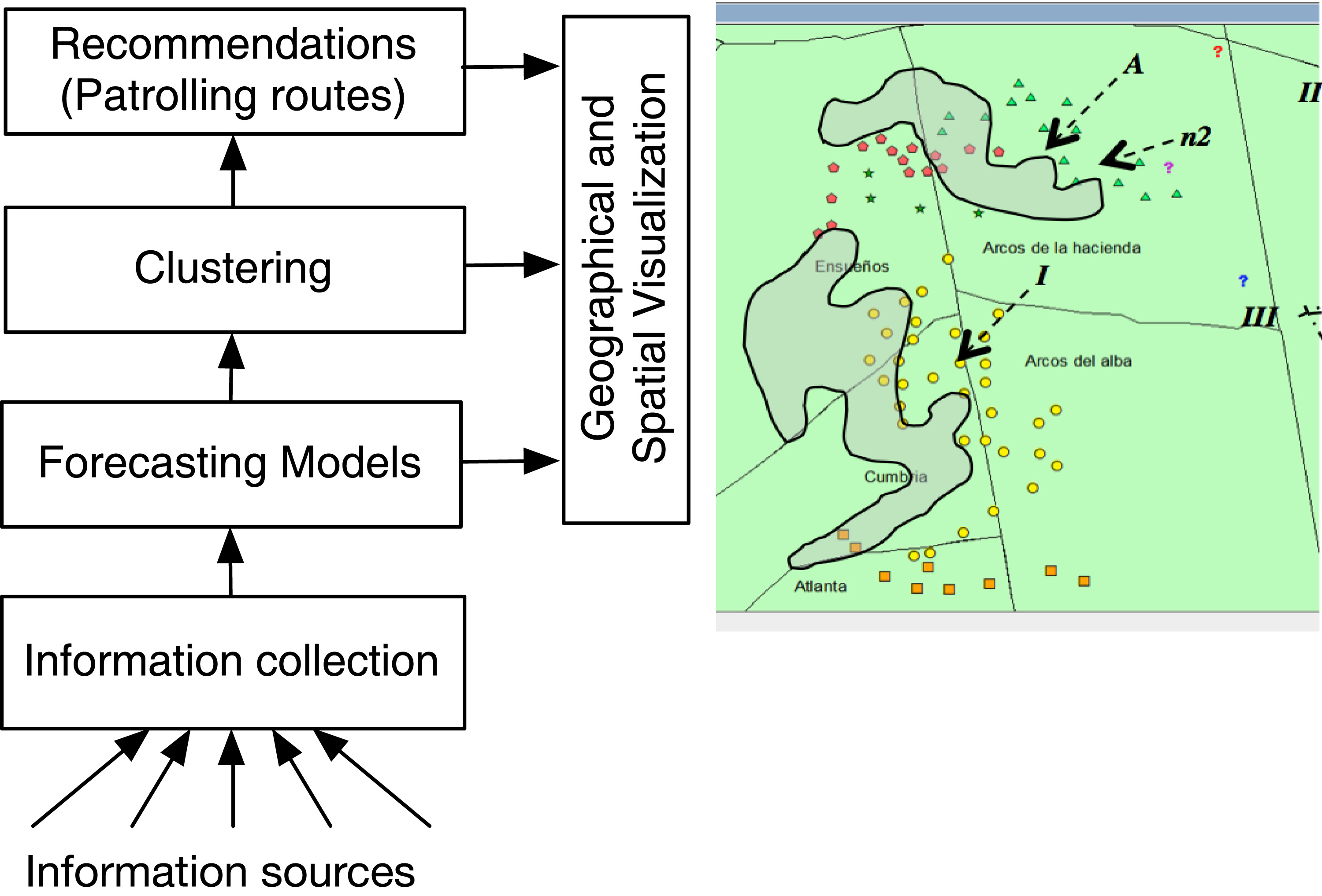

1.1 Proposed model

The forecasting, clustering and routing model reported here is a framework designed to prevent and react to crime. This framework is made-up by several layers as shown in Fig. 1.

The function of the first layer is to gather, standardize and analyze data from six established information sources. In terms of pattern recognition, layer one constitutes the supervision sample. The second layer contains several prediction algorithms (see Section 2). The input to the third layer is the set of predictions made by the algorithms of the previous layer and it identifies, clusters and maps important hotspots (see Section 3). The fourth layer generates recommendations for addressing the forecasted scenarios. Particularly in this paper we discuss the patrolling recommendations (see Section 4).

Careful structuring of the input data is of utmost importance, so that the forecasting model can be efficient and has an acceptable level of precision [13]. The problem of crime prediction and recommendation generation requires several different information sources, all of them directly related with public security, but not easily accessible. For this project, we have chosen six information sources arranged into four categories as follows: information on (1) crimes committed, (2) citizens’ reports, (3) resources and police activities, and (4) socioeconomic data of the region under study. In each of these categories, information should be precisely located in time and space. For our study, we use data from the municipality of Cuautitlán Izcalli, State of Mexico and data from the Sacramento California (CA) Police Department.

2. Forecasting criminal activity

There are several works devoted to the study of spatial and temporal decisions made by criminals, i.e., identifying hotspots where criminal activity is concentrated – see [1, 2, 8, 26, 31, 33, 35, 36, 37, 39]. A widely used method is the Spatial and Temporal Analysis of Crime program (STAC) [5], which clusters crime points within ellipses [3]. Jefferis [24] surveys additional hotspot methods, the most sophisticated of which employs a kernel density estimation method [27]. Nevertheless, the main disadvantage of statistical methods is that they do not offer additional semantic information for describing the phenomenon under study. In the specific case of crime prediction, this kind of information is highly desirable, as it is needed to support decision-making processes and, in general, to prepare preventive and corrective policies. Because of this, we have selected inductive classification methods over statistical ones in order to generate an inductive description of each type of criminal activity studied. These descriptions by themselves constitute valuable information that provides a general overview of the criminal activity scenario. Furthermore, by using these inductive definitions, it is possible to identify the expected increase or decrease in specific criminal activities that will most likely occur in specific geographic areas and times.

This section deals with the design of the forecasting model within the proposed framework of criminal activity analysis within a specific time period and location using several different supervised classification techniques. W present details of our forecasting model, from general Forecasting with Inductive Supervised Classification (Section 2.1) to our particular implementations of CR- $\Omega+$ (Section 2.2) and (CR- $\Omega$ $+$ M) with general discrimination [21] (Section 2.3).

2.1 Forecasting with inductive supervised classification

One of the most interesting tasks of the Pattern Recognition discipline is the study of forecasting models [10, 30]. The forecasting problem can be treated as a classification problem; this allows taking advantage of the large number of available classification algorithms. The great majority of current forecasting models has a statistical nature and is mainly devoted to time series analysis (for an exhaustive review of these methods, refer to [10, 22]). As stated previously, we are interested in the particular semantics of crime analysis, so we propose an inductive forecasting model.

The forecasting model is expressed as a supervised classification problem in the following terms: Given a database containing a set of patterns corresponding to crimes perpetrated within the region under study that are spatio-temporally labeled, group such patterns into crime families, where a crime family consists of all the crime patterns corresponding to similar crimes that are fought with the same resources. These families form the supervision sample to be used by the classification algorithms. Afterwards, a learning process is carried out to describe each family in both positive and negative ways. In order to predict a specific criminal scenario (i.e., the time, location and type of criminal activity to be predicted), a pattern containing all the relevant data is constructed and submitted for classification in accordance to the previously assembled supervision sample. The classification algorithm gives as a result the degree of membership of such a pattern to each one of the established families. Consequently, each degree of membership is interpreted as the forecasted increase or decrease in the criminal activity for the specified time and location.

To make forecasts, a careful design of the classification problem semantics is required. Specifically, this includes three basic aspects of the problem: (1) the objects under study and the attributes or features that will be used to describe them; (2) the number of classes and how patterns will be classified; and (3) what kind of learning the classification algorithm will use. Each one of these aspects is discussed below.

2.1.1 Objects and descriptive features

The objects under study are either criminal activity scenarios or citizens’ reports recorded in each geographical area at a given time. Temporal information includes the date and time components, whilst the location refers to the area in which the criminal activity was recorded. For each one of the studied scenarios an $r$ -dimension pattern is defined containing all the data available. The resulting set of these patterns forms the supervision sample.

We perform two different modes for analyzing the criminal data, considering two different semantics for the crime families to be identified.

The first mode groups the supervision sample patterns into three classes that indicate the kind of environment in which the criminal activity was recorded. These three classes represent criminal activities committed in: (1) public roads and highways; (2) homes; (3) stores and shops.

The second mode groups the patterns into four classes based on the kind of social impact that the criminal activity has. These four classes are: (1) robbery in all its modalities; (2) homicide; (3) injury; (4) property damage.

These groupings were selected considering the main goal of the project, which is to provide recommendations, particularly aimed to patrolling routes, to the public security authorities. Based on the recommendations of our system, authorities will have information to spawn direct actions to prevent the crimes perpetrated in public streets, shops, homes, or industries.

2.1.2 Learning

We use information regarding the crimes committed and reported to the Public Prosecutor’s office. The data corresponding to the crimes committed during a certain time can be used to test the proposed forecasting model. After having initially debugged the information provided by the Public Prosecutor’s office, a supervision sample containing the space-time location of the crimes committed is build. A classifier learning process is trained on data containing a good distribution of crime patterns across the three or four classes mentioned above, depending on the mode under investigation. This learning process consists of constructing inductive definitions that describe in positive and negative ways the patterns contained in each one of the classes in the supervision sample. The inductive definition $\theta$ corresponding to each $C_{i}$ class, is an expression of the form:

$\theta\left(C_{i}\right)=\bigcup{P_{m}\left(C_{i}\right)}$ (1)

where each $P_{m}(C_{i})$ is a property identified among the patterns pertaining to the $C_{i}$ class [6]. The properties are subsets of descriptive features associated with specific values. For each class, a positive $\theta^{+}(C_{i})$ and a negative description $\theta^{-}(C_{i})$ are made. Once the descriptions are obtained, we can use an inductive classification algorithm.

2.2 The classification algorithm

We use a combination of the Kora- $\Omega$ algorithm proposed in [21], which is an extension of the KORA-3 [6, 17, 16, 15] algorithm and the Representative Sets (CR $+$ ) algorithm [3, 9], which both share the notion of property in the form of a subset of features associated with specific values in these features.

A $P_{m}$ property identified in the $C_{i}$ class has the form shown in Eq. 2.

$P_{m}=\left[{\begin{array}[]{*{20}c}x_{p},\ldots,x_{q}\\ \langle v_{p}\rangle,\ldots,\langle v_{q}\rangle\\ \end{array}}\right]$ (2)

Where $x_{i}=p,\ldots,q$ are features used to describe the objects under study and each $\langle v_{j}\rangle$ , $j=p,\ldots,q$ is a specific value in the domain of the $x_{j}$ feature observed among the patterns in the $C_{i}$ class.

2.3 CR-

\Omega+

with general discrimination (CR-

\Omega

+

The CR- $\Omega+$ Modified Algorithm (henceforth referred as CR- $\Omega$ $+$ M) is based on the previous algorithm, modifying the counting of features present in other classes, i.e., those related with the ${\beta}_{1}^{\prime+}$ and ${\beta}_{1}^{\prime-}$ thresholds.

For the previous algorithm, $\the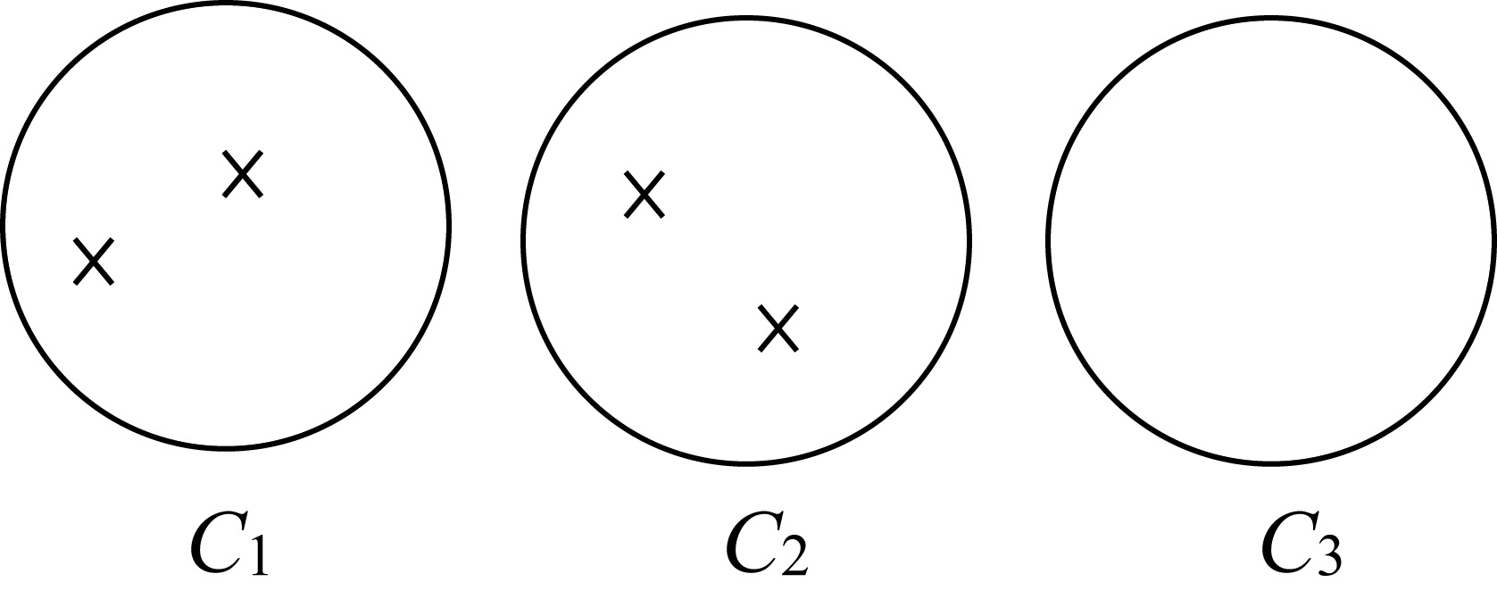ta_{1}^{+}\left(C_{i}\right)$ was calculated by counting a feature set present at least $\beta_{1}^{+}$ times in $C_{i}$ and no more than ${\beta}_{1}^{\prime+}$ times in any other class $C_{j}$ with $j\neq i$ . For the CR- $\Omega$ $+$ M algorithm, we modify this last part, now requiring “no more than ${\beta}_{1}^{\prime+}$ times in the union of other classes $C_{j}$ with $j\neq i$ ”, that is, $\bigcup C_{j},j\neq i$ . The same occurs for calculating $\theta_{1}^{-}\left(C_{i}\right)$ requiring now that the feature set be present at least $\beta_{1}^{-}$ times in $\bigcup{C_{j}},j\neq i$ and no more than ${\beta}_{1}^{\prime-}$ times in $C_{i}$ .

Figure 2.

The CR- $\Omega+{\rm M}$ Classification Algorithm will consider the X features as negative for class three with $\beta_{{1}}^{{-}}=3$ , whereas the CR- $\Omega+$ algorithm will not.

In Fig. 2 we exemplify the effect of this modification. Given a threshold $\beta_{1}^{-}=3$ for $C_{3}$ the feature $X$ in the first algorithm (CR- $\Omega+$ ), $\theta_{1}^{-}\left(C_{3}\right)$ would be empty, whereas for the CR- $\Omega+{\rm M}$ algorithm, the cardinality of the features would be 4, yielding $\theta_{1}^{-}\left(C_{3}\right)=\{X\}$ .

Once the classifiers are trained, it is necessary to cluster the spatiotemporal features in order to visualize and find important hotspots. This is discussed in next section.

3. Clustering criminal activities

We used an approach based on Nath [32]. He uses a $k$ -means algorithm is used for identifying crime patterns – a crime pattern is described as a specific group of criminal actions with similar MO characteristics. He calls a group or cluster of crimes, a pattern. He shows results of experiments made on a small sample of data, shown in Table 1.

Table 1
Example of criminal data [32]

Crime type	Suspect’s race	Suspect’s sex	Suspect’s age gr	Victim’s age gr	Weapon
Robbery	B	M	Middle	Elderly	Knife
Robbery	W	M	Young	Middle	Bat
Robbery	B	M	?	Elderly	Knife
Robbery	B	F	Middle	Young	Piston

By applying a $k$ -means clustering algorithm to the datasets, the author groups crimes with similar MO. He explains that in the robbery sample (shown in Table 1) pattern behavior may be observed in rows 1 and 3, where the suspect’s description matches, as well as the victim’s profile. However, no explanation is given about the intra-class diversity of the crimes, and why the author used k-means as the clustering algorithm of choice. Figure 3 exemplifies the results published by Nath.

Figure 3.

Nath’s results excerpt [32].

For the clustering layer, we propose the use of a clustering technique based on pattern density, together with a space-time similarity function to identify areas with high concentration of crime (hot-spots). Then we compare the results obtained with our similarity function with those obtained by the proposed similarity function used in the original paper of the ST-DBSCAN algorithm [4]. The comparison criteria used by the space-time similarity function and its specific use to cluster criminal activities are the main contributions of this clustering method.

3.1 Proposed model

The purpose of using density-based clustering techniques in the context of crime-analysis is to achieve a non-statistical identification of the observed spatial and temporal trends in the commission of crimes, as well as to isolate exception cases that do not fit into those trends. This information is useful for the crime-analyst in order to develop specific strategies, both to fight and prevent delinquency, in the middle and long terms.

3.1.1 Pattern representation

We consider the crime-pattern output from the previous layer as the abstract representation of a single criminal phenomenon. This crime-pattern consists of three main components: crime specifics, space, and time; all three related to the perpetration of a specific crime. This allows the specialist to identify periods of high criminal activity and their geographic location. Therefore, the components of a criminal pattern are the following:

Crime specifics: It indicates the specific type of crime committed as well as many of its characteristics, such as the level of violence, number of persons implicated, types of weapons, modus operandi, etc.

Table 2
Data sample (out of 80 patterns) of the burglary dataset

Weapon	Location	Date
Firearm	Ensueños	22/08
Not specified	Cumbria	21/08
Sharp instrument	Arcos de la Hacienda	13/09
Banned weapon	San Isidro Labrador	01/03

Figure 4.

Criminal data referred to the geographic area where they were committed. Each red spot represents a crime incident of the “burglary” type.

Space Location: Geographic area where the crime was committed. This feature may be observed at different levels of detail: state level, patrolling sector, residential development or even street and number. Time Location: Time when the crime was perpetrated. In this component, as well as in the one mentioned above, several levels of detail are possible: year, month, date or even the time of the day. Each one of these components may consist of one or more variables that will be called pattern features that provide a higher level of detail to the pattern. A crime-pattern (D) has the following structure:

$\displaystyle D=(\langle\textit{crime specifics}\rangle,\langle\textit{space % location}\rangle,\langle\textit{time location}\rangle)$

The trend-identification process starts by analyzing a set of crime-patterns, each one with the same level of detail and within a limited geographic location, occurred within a given time interval. Table 2 contains a sample of burglary patterns obtained from the Cuautitlán Izcalli area, in the State of Mexico.

Figure 4 shows how such patterns are plotted in the map of the corresponding area divided into surveillance sectors.

In Table 3 we show another sample of the same dataset with a different level of detail from the one shown in the former sample. The differences between the two sets can be observed on the temporal and crime specific components of the patterns. This second set contains robbery-patterns and their location is another surveillance center within the same district of Cuautitlán Izcalli, Mexico.

Table 3

Data sample (out of 126 patterns) from the robbery data set

Robbery type	Weapon	No. of members	Location	Month
Break-in	Sharp instrument	2	El Rosario	DEC
Auto-parts theft	Without weapons	4	Adolfo López Mateos	FEB
Robbery to passer-by	Firearm	3	El Rosario	FEB
Robbery to passer-by	Sharp instrument	1	Cofradía-III	DEC

The complete first dataset (burglary) contains 80 patterns, while the second one (robbery) contains 126 patterns.

3.1.2 The ST-DBSCAN algorithm.

Briant and Kut [4] describe an extension of the DBSCAN algorithm for spatio-temporal clustering, called ST-DBSCAN. This extension proposes the separate calculation of space and time similarities between patterns.

The ST-DBSCAN algorithm requires, besides the dataset to be processed, the following two parameters: the minimum number of neighbors around an object to consider a high density situation, which will be called MinPts; and the radius of the neighborhood which will be called Eps.

3.1.3 Density-based clustering

Density-based clustering algorithms can group patterns with a high spatial concentration within a delimited region isolating in the processes those patterns with a low degree of spatial similarity, which are regarded as non-related appearances of criminal activity. In this project, we used the ST-DBSCAN algorithm, an extension of DBSCAN to work with space-time components [4]. This algorithm was implemented as originally described except for the similarity function. Our proposed spatial comparison criteria and similarity function (Section 3.1.4, Eq. 3) were substituted in place of the original ones based on Euclidean distance and sector division.

3.1.4 Space comparison criterion and the similarity function

The comparison between patterns is achieved by a similarity function formed by the weighted sum of a set of comparison criteria (Cc) normalized according to the number of features that form the pattern. Each of these comparison criteria measures the similarity of each feature that makes-up the pattern. The way in which the similarity of the space component is measured is shown below.

Figure 5 shows an area divided into four surveillance sectors. A surveillance sector is a geographic zone made up by location (residential developments) and it is defined by the police department for the allocation of financial resources. According to the space comparison criterion based on Euclidean distance, patterns belonging to the same sector but separated by a long distance will not be similar (See Fig. 5(a), patterns p4 and p6), while patterns which are geographically close to each other, even if they belong to different sectors, will be considered as similar, see Fig. 5(a), patterns: p1 and p2.

Figure 5.

Surveillance sectors. (a) Euclidean comparison; (b) Comparison by sector division.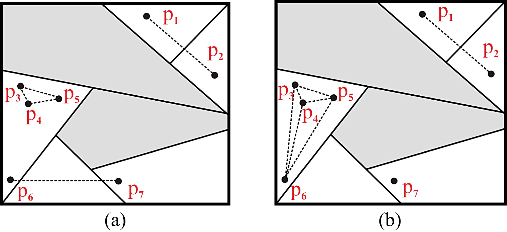

The spatial comparison criterion based on regions divided by surveillance sectors, strongly suggests that the maximum space-similarity should be achieved by patterns belonging to the same sector (See Fig. 5(b), patterns: p3 to p6), followed by patterns belonging to contiguous sectors (See Fig. 5(b), patterns: p1 and p2). This kind of clustering yields much more useful clusters because patrolling routines, as well as investigative teams usually schedule their operations by sector. Of course, different comparison criteria can be considered depending on the needs by each crime-analyst.

Our proposed similarity function is defined by the following equation:

$f\left(O_{i},O_{j}\right)=\frac{1}{r}\sum\limits_{s=1}^{r}\left(\propto_{s}{Cc% }_{s}\left(O_{i},O_{j}\right)\right)$ (3)

Where: $r$ is the number of features that make up the pattern. $o_{i},o_{j}$ are the patterns being compared. $\alpha_{s}$ is the weighting factor of feature $s$ . $Cc_{s}(∼{})$ is the space-time and attribute comparison criteria for feature $s$ .

Experiments in Section 5 will show that this similarity function based on our space comparison criterion produces better results than the space comparison criterion based on Euclidean distance. Once data is properly clustered, important hotspots can be identified. These hotspots are in turn surveillance points that must be considered in a patrolling route. The next section will deal with the construction of such routes.

4. Route patrolling

Several methods have been developed for tackling the problem of route optimization. The field of multi-robot cooperative tasks provides an interesting set of examples; see [1] for a thorough compendium of several models. Within this approach, we found two major drawbacks. The first one is that some of them are designed for small devices [34], and the second one is that they are designed for automatic execution, and usually they do not allow incorporating certain restrictions pertaining to real world human driving and wide area sectorization. Other approaches are based on workload balancing models [40], local search techniques [43], and agents [7]. However, to our knowledge, ant colony systems, while being known to be effective for finding optimal routes [42, 20], have been scantly applied to police patrol route planning considering three real needs:1

¹
Direct communication by the personnel of the Emergency Central C4 of the municipality of Cuautitlán Izcalli.

(a) finding the optimal route for a patrol to attend an emergency call; (b) finding the optimal route between the current location of a patrol and a set of nearby streets that require surveillance; and finally (c) to find the optimal route for a patrol, so that it can survey different points of major criminal incidence in a specified neighborhood. In the next Section 4.1, we will present a short introduction to ant colony systems, then in Section 4.2 we describe our proposed method.

4.1 Ant Colony Optimization

Ant Colony Optimization algorithms are models inspired in real ant colonies. Studies show how animals that are almost blind, such as ants, can follow the shortest path to their supplies (food) [11]. This is due to the exchanging information ability ants have, since each one of them, while moving, leaves a trace of a substance called pheromone along their path. Thus, while an isolated ant moves essentially in a random way, agents of an ant colony detect the pheromone trace left by other ants, and tend to follow such trace. These ants, in turn, leave their own pheromone along the travelled path, making it more attractive, since the pheromone trace has been reinforced. With time, the pheromone evaporates, causing the trace to weaken. In short, it could be say that the process is characterized by a positive feedback, in which the probability for an ant to choose a path increases with the number of ants that previously have chosen the same path. One of the first known applications of the ant colony system was the travelling salesman problem (TSP) [18], obtaining favorable results. From that algorithm, several heuristics have been developed to improve the original algorithm, and have been applied to other problems such as the vehicle routing problem (VRP) [14] and the Quadratic Assignment Problem (QAP) [29].

In this section, we present results of a heuristic based on an improved version of the ant colony optimization (ACO) algorithm called MMAS (Max Min Ant System) [41].

The ACO algorithms are iterative processes. In each iteration, a colony of $m$ ants is deployed, and each one of the ants constitutes a solution to the problem. Ants build solutions in a probabilistic way, being guided by a trace of artificial pheromone, and by information calculated a priori in a heuristic way. The probabilistic rule for traversing nodes on a graph is:

$p_{ij}^{k}\left(t\right)=\frac{\left[\tau_{ij}(t)\right]^{\alpha}\cdot\left[% \eta_{ij}\right]^{\beta}}{\sum\limits_{l\in N_{i}^{k}}{\left[\tau_{il}(t)% \right]^{\alpha}\cdot\left[\eta_{lj}\right]^{\beta}}}$ (4)

where $p_{ij}^{k}\left(t\right)$ is the probability, in a $t$ iteration of the algorithm, the $k$ ant currently situated in city $i$ , chooses city $j$ as the next stop. $N$ is the set of cities not yet visited by the ant $k$ . $\tau_{ij}(t)$ is the amount of pheromone accumulated on the arc ( $i, j$ ) of the network at the $t$ iteration. $\eta_{ij}$ is the heuristic information for which, in the case of TSP, the inverse of the distance between $i$ and $j$ cities. $\alpha$ and $\beta$ are parameters of the algorithm to be adjusted.

When all ants have built a solution, pheromone must be updated on each arc. The formula for this is:

$\displaystyle\tau_{ij}\left(t+1\right)=\left(1-\rho\right)\cdot\tau_{ij}\left(% t\right)+\Delta\tau_{ij}^{\textit{best}},$ $\displaystyle\Delta\tau_{ij}^{\textit{best}}=\begin{cases}{\displaystyle\frac{% 1}{L^{\textit{best}}}}&\text{if the arc $\left(i,j\right)$ belongs to $T^{% \textit{best}}$}\\ 0&\text{otherwise}\\ \end{cases}$ (5)

Where $\rho$ is the pheromone evaporation coefficient. $T^{\textit{best}}$ can be the best solution found at the moment, or the best solution found in the current iteration. The level of pheromone should be in a range $\left[T_{\min},T_{\max}\right]$ These limits are established in order to avoid stagnation in the search of solutions. All pheromone is initialized with $T_{\max}$ . After updating the pheromone, a new iteration can be started. The final result is the best solution found over all iterations.

This gives us a global view of the MMAS algorithm. In the next section, we will present its application to the problem of human and material resources for patrolling routes. We aim to a three-folded purpose: (a) To find the optimal route between a patrol’s current location, and a point where a call for help has been raised. (b) To find optimal routes for patrolling a small set of nearby streets in a neighborhood, and finally (c) to find optimal routes for patrolling different points of major criminal incidence in a specified neighborhood.

4.2 Proposed method

We will illustrate our methodology with the example case of a neighborhood of the municipality of Cuautitlán Izcalli, Mexico. This neighborhood was selected considering the current geographic level for assignment of patrolling routes. In Fig. 6 the structure at street level can be seen. Patrols must cover the points considered as the most important ones.

Figure 6.

Structure showing streets of a neighborhood in Cuautitlán Izcalli, Mexico.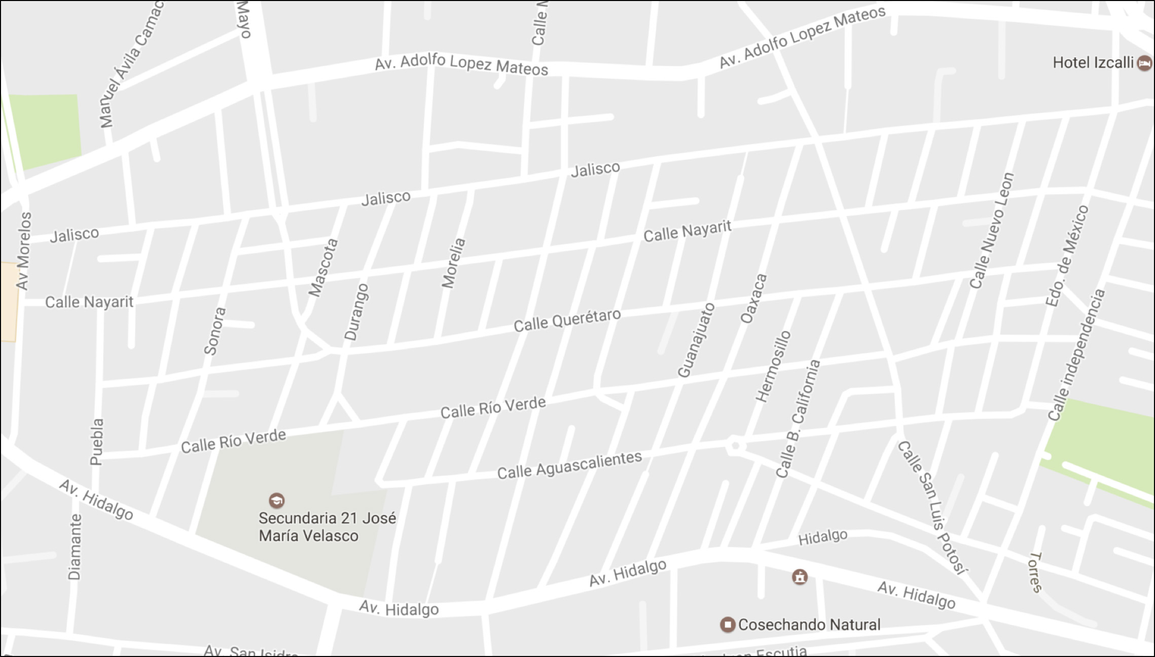

Then, the street structure is transformed to a directed graph $G=(V,E)$ , where $V$ is a set of vertices or nodes [25]. In our case, those are the crossings between streets. See Fig. 7. $E$ is a set of arcs connecting the set of nodes, and represent the streets conforming the neighborhood. Each one of these represents the direction a street has. The obtained final graph can be seen in Fig. 7.

Figure 7.

Graph obtained from street structure from a real neighborhood.

Our solution employs the algorithm MAX-MIN Ant [41] with modifications to the original restrictions for the TSP for which it was originally presented. Compared to the original TSP, we are interested on having $N$ ants with certain routes that represent the number of available units. In the original problem, we have only one individual. We adapted the MMAS as shown in Fig. 8.

5. Experiments and results

Following the architecture of our framework shown in Fig. 1, in this section we will present results of each one of the layers applied to real data of a national municipality in order to validate their effectiveness. For the forecasting model (Section 5.1), we will compare two inductive classification methods (namely the CR- $\Omega+$ and its variation CR- $\Omega+$ M) against a traditional KORA- $\Omega$ classifier. Then, we will compare the tendency of our prediction using RMSE against a Bayesian forecasting method. For the clustering model (Section 5.2) we implemented the ST-DBSCAN with a standard Euclidian distance measure, and then we compare its results with our proposed measure based on sector space division. Finally, for the patrolling route recommendations (Section 5.3), we compare our proposed method with a random walk algorithm.

5.1 Forecasting

In the Cuautitlán Izcalli district, located in Mexico, the local Government launched the Centro de Emergencias Cuautitlán (CERCA, Cuautitlán Emergency Center) in 2007. An important part of its function is the gathering of the information corresponding to the three first categories of information sources. Therefore, this district was selected as a case study and test field for the forecasting, clustering, and patrolling recommendation model reported herein.

We perform two analyses: punctual hotspot prediction (Sections 5.1.1 and 5.1.2), and tendency analysis (Section 5.1.3). For the first analysis, we use data from the municipality of Cuautitlán Izcalli, State of Mexico. Within this analysis, we perform experiments for spatial and temporal location of crime (Section 5.1.2.1) and expected family of crime (Section 5.1.2.2). For the tendency analysis (Section 5.1.3) we use data from the Sacramento California (CA), police department.

Table 4
Pre-processed report used as input to the algorithms – Mode 1

Time quadrant	Date	Residential zone	Pub. road (Class 1)	Home (Class 2)	Shops (Class 3)
Q8	Jan	Arcos del Alba	1	0	0
Q4	Apr	Atlanta	1	0	0
Q1	Jun	Bosques de la Hda.	0	1	0
Q6	Apr	Bosques del Lago	0	1	0
Q6	May	Centro Urbano	0	1	0
Q5	Mar	Hacienda del Parque	0	0	1
Q5	Jun	Infonavit Norte	0	0	1

Figure 8.

Pseudocode for the MMAS algorithm. Asterisks show the steps to be modified for the random walk baseline comparison.

5.1.1 First analysis: Punctual hotspot prediction

In this Section, we describe the details of our experimentation for applying the different algorithms presented in previous sections to the two modes mentioned in Section 2.1.1. All experiments in this section use data from January 1 ${}^{\rm st}$ 2007 to July 31 ${}^{\rm st}$ , 2007 from the municipality of Cuautitlán Izcalli, State of Mexico. In total, there were 1551 records. Not every record from the original sample was useful due to incompleteness or ambiguity when classified on the chosen relevant classes; for many records, there was no precise information about the place where the crime was perpetrated.

Crimes were grouped by kind in different classes, as aforementioned in Section 2.1.1, for two different modes:

1.
(1) public roads and highways; (2) homes; (3) stores and shops.
2.
(1) robbery in all its modalities; (2) homicide; (3) injury; (4) property damage.

Data are represented as shown in Table 4, accordingly to Mode 1, and in Table 5, accordingly to Mode 2. For the first mode, we used only 205 from 1551 records because the remaining records did not have enough information to distribute them amongst the classes selected. For the second mode, we were able to use all records. We will use this information as the input of the KORA- $\Omega$ , CR- $\Omega$ , and CR- $\Omega+$ algorithms. The results of the classification of both analyses are reported in the following sections.

Table 5
Pre-processed report used as input to the algorithms – Mode 2

Time Date Residential zone Robbery Injury Homicide Property damage

quadrant (Class 1) (Class 2) (Class 3) (Class 4)

Q8 Jan Arcos del Alba 1 0 0 0

Q4 Apr Atlanta 1 0 0 0

Q1 Jun Bosques de la Hda. 0 1 0 0

Q6 Apr Bosques del Lago 0 1 0 0

Q6 May Centro Urbano 0 0 1 0

Q5 Mar Hacienda del Parque 0 0 0 1

Q5 Jun Infonavit Norte 0 0 0 1

5.1.2 Results of punctual hotspot prediction

Time	Date	Residential zone	Robbery	Injury	Homicide	Property damage
Q8	Jan	Arcos del Alba	1	0	0	0
Q4	Apr	Atlanta	1	0	0	0
Q1	Jun	Bosques de la Hda.	0	1	0	0
Q6	Apr	Bosques del Lago	0	1	0	0
Q6	May	Centro Urbano	0	0	1	0
Q5	Mar	Hacienda del Parque	0	0	0	1
Q5	Jun	Infonavit Norte	0	0	0	1

In this section, we present the results of our two first experiments, consisting on applying the previously presented algorithms following the two modes mentioned in Section 2.1.1.

5.1.2.1 First experiment: Location of crime

Mode 1 has three classes: (1) public roads and highways; (2) homes; (3) stores and shops. Using the KORA- $\Omega$ Algorithm we calculate the characteristic features and the complementary features of the sample applying it to a set of data with 160 patterns ( $\sim$ 78% of the 205 records from the whole sample); these 160 records were spread in the following way: Public roads: 105, Home: 35, Stores: 20. The learning percentage of the algorithm for the known data is 88%. To calculate the prediction rate, we used a sample of 45 patterns ( $\sim$ 22% of the 205 records from the whole sample) divided as follows: 30 patterns for crimes in public roads, 8 patterns for home crimes, and 7 patterns for shop crimes. The algorithm had an effectiveness of 66% for the test set.

We used the CR- $\Omega+$ Algorithm on the same 160 patterns applied in the previous experiment. The learning percentage of the algorithm for the known data rose to 92.5%. For prediction rate, we used the same 45 patterns for test from the previous experiment. The algorithm had a prediction rate of 69% of for the real data test set. This means that it was possible to predict in more than two thirds of cases the place where crimes are likely to have a greater incidence.

Table 6
Comparison of recall measures

Recall	CR- $\Omega+$ (2 $+$ Features)		CR- $\Omega+$ M (2 $+$ Features)		CR- $\Omega+$ (1 $+$ Features)		CR- $\Omega+$ M (1 $+$ Features)
	Train		Test		Train		Test
I. April 2007	77.0%	22%	78.0%	23%	77.0%	24%	77.0%	24%
II. July 2007	79.0%	23%	77.0%	30%	77.0%	29%	77.0%	30%
III. April 2008	79.0%	23%	79.0%	21%	79.0%	23%	77.0%	24%

5.1.2.2 Second experiment: Crime families

One of the main disadvantages depicted in the first analysis is the low number of records that can be used for prediction, although this allowed predicting the place where crimes are more likely to be perpetrated. For this experiment, we grouped the sample data in the following classes: (1) robbery in all its modalities, (2) homicide, (3) injury, and (4) property damage. This analysis allows using 1231 records out of 1551. For the sake of considering the heterogeneous distribution of the data between different dates, we tested the algorithms against:

150 new events corresponding to the month of April of 2007.

123 new events corresponding to the month of July of 2007.

321 new events corresponding to the month of April of 2008.

In contrast with the previous experiment, where the 1551 records from January 1 ${}^{\rm st}$ 2007 to July 31 ${}^{\rm st}$ , 2007 were split in 78% for training and 22% for testing, in this experiment we used 100% of such data as training, and the additional patterns of I, II and III as different tests. Note that these new events were not included in the previous records. The purpose of testing against different test sets is to examine the performance of the algorithm given the heterogeneity of the provided data. It can be seen, for example, that the newest data from April 2008 has the double the number of records compared to data from previous dates (April of 2007, and July of 2007).

5.1.2.3 Results

Table 6 shows the results in terms of recall of applying the algorithms CR- $\Omega+$ and CR- $\Omega+$ M algorithms to the different test sets. We also explore limiting the number of features in a feature set to at least two, and applying no limitations (so that feature sets can be composed of only one feature). For all experiments, the empirically chosen values for beta were: $\beta_{1}^{+}=3,\beta_{1}^{\prime+}=1,\beta_{1}^{-}=3$ and $\beta_{1}^{\prime-}=1$ , $\beta_{2}^{+}=0$ , $\beta_{2}^{-}=3$ for CR- $\Omega+$ , and $\beta_{2}^{-}=1$ for CR- $\Omega+$ M.

The CR- $\Omega+$ classifier was tested by classifying patterns previously not contained in the supervision sample [3]. We compared results against those achieved using the standard KORA- $\Omega$ algorithm, and obtained an improvement for the learning rate, as well as for the test rate. The original KORA- $\Omega$ algorithm obtained 88% and 66% for learning rate and test rate, respectively, whereas the proposed CR- $\Omega+$ algorithm obtained 92.5 and 69%, respectively when classifying data into the following classes: (1) public roads, highways, (2) homes, (3) stores and shops. This suggests that we are able to predict the kind of crime spatially and temporally for two out of three crimes. We evaluated with test data for crimes perpetrated from January 1 ${}^{\rm st}$ 2007 to July 31 ${}^{\rm st}$ , 2007. Approximately 78% was used for training and approximately 22% for testing.

In our second analysis, we used the whole data set from January 1 ${}^{\rm st}$ 2007 to July 31 ${}^{\rm st}$ for training, while we selected three different data sets for testing: (I) 150 patterns corresponding to the month of April of 2007, (II) 123 patterns corresponding to the month of July of 2007 and (III) 321 patterns corresponding to the month of April of 2008. We used three different datasets to evaluate the homogeneity of the data. We obtained 77% recall in learning rate (up to 87% in precision), and 30% recall in forecast. This suggests that we are able to predict punctually the kind of crime, given a spatio-temporal location, at least for one of each four crimes perpetrated.

We have shown how both algorithms, the CR- $\Omega+$ and its variation CR- $\Omega+$ M, perform better than the classical algorithms (KORA- $\Omega$ ). Particularly, it can be seen from Table 6 that the CR- $\Omega+$ M improves in general the forecast recall – for example, for test II, using 2 $+$ features, it raises recall from 23% to 30%.

5.1.3 Tendency analysis

In order to compare with other related systems, we performed tests with a different dataset and compared against predictions using a Naïve Bayes classifier. We compare results using the Spatio-Temporal Root Mean Square of Errors (STRMSE) measure proposed by Ivaha et al. [23] with the Naïve Forecasting Method (NFM) described as well in [23]. The STRMSE measure consists of daily measurements of forecast errors, and it is based on the root mean squared error, divided by the number of days of the sample. Two or more models may be compared using STRMSE as a measure of how well they explain a given set of observations: the unbiased model with the smallest STRMSE is generally interpreted as best explaining the variability in the observations. STRMSE is calculated as shown in Eq. 6. $n$ is the total number of days forecasted and $m$ is the total number of samples.

$\textit{STMRSE}=\sqrt{\frac{1}{n}\sum\limits_{i}^{m}\frac{(O_{i}-\hat{O}_{i})^% {2}}{m}}$ (6)

To test the proposed forecasting algorithm, we used the Sacramento dataset. This dataset contains 152,812 registered crimes and was made available by the Sacramento CA, police department.2

http://www.sacpd.org/crime/stats/reports/.

All crimes were committed within 19 surveillance sectors (space-units), over a period from January 2004 to December 2008 (time-units).

By analyzing only records from the last five years (2004 to 2008), a forecast was calculated for time-unit January 2009, all registered crime-families and within all 19 surveillance sectors. The foretold number of crimes was then compared with the real-life police-registers from that same space-time unit (2,219 crimes during January 2009).

5.1.3.1 Results

Using the aforementioned method, all positive and negative characteristic space-time properties for each crime-family were found. For the training set from 1/1/2004 to 31/12/2008, and test set from January 2009, the STMRSE of the Bayes (NFM) forecast was 7.05, while ours was 0.90. A similar behavior was observed for the test set of February 2009 (using the same training set): Bayes STMRSE yielded 8.45, while we obtained 0.97. We can (indirectly) compare with the system presented by Ivaha et al. [23]. His results are shown in Table 7, along with ours. NFM is the Naïve Forecasting Method, OLS-NI is the Ordinary Least Square method on Number of Incidences, and OLS-PC is the Ordinary Least Square method on Percentages of Crime (OLS-PC). For details on how NFM, OLSI-NI and OLS-PC results are obtained, please refer to [23].

Table 7

Comparison with the systems presented by Ivaha et al.

	NFM	OLS-NI	OLS-PC	Ours
STMRSE	1.57	1.139	1.131	0.97

These results show that the proposed method has very high effectiveness, with an STRMSE below 1.0 forecasting all space-units, during January 2009 (with a total of 2,219 crimes). This means that, in average, the proposed method only fails in less than five occurrences of each crime-family. Such precision is fairly acceptable for automated crime-analysis systems and might constitute a useful tool for planning preventive police operations.

5.2 Results of clustering

The values of Eps and MinPts in our implementation of ST-DBSCAN were calculated with Eqs 7 and 8:

$\textit{Eps}=1-\min(f(o_{i},o_{j}))$ (7)

where $f$ ( $o_{i}$ , $o_{j}$ ) is the similarity function with $i=1,2,\ldots,n;j\neq i$ . $n$ being the total number of patterns.

$\textit{MinPts}=|O|+1$ (8)

where: $|O|$ is the cardinality of the pattern.

The first experiment was conducted over the burglary dataset. For this experiment the feature called weapon is the most relevant attribute, so the best result is deemed to be the one that groups criminal incidents committed with the same weapon.

A very important aspect to be considered is the clarification of the difference between the patterns identified as noise and the outliers in the dataset. Noise refers to those patterns that may be spatially similar to other patterns or groups, but do not share other similar characteristics, while an outlier is a pattern geometrically separated from other patterns or groups. This clarification is necessary because the ST-DBSCAN identifies noise.

The results generated by the Euclidean space similarity function vs. our proposed space competition criteria are shown in Fig. 9. Type of crime is described by different geometric shapes, described in Table 8. In both parts (Figs 9(a) and (b)) the patterns labeled by question signs represent noise patterns (elements that do not have characteristics similar to others).

Figure 9.

ST-DBSCAN results: (a) with Euclidean space similarity function (left), (b) with space similarity function based on sector division (right).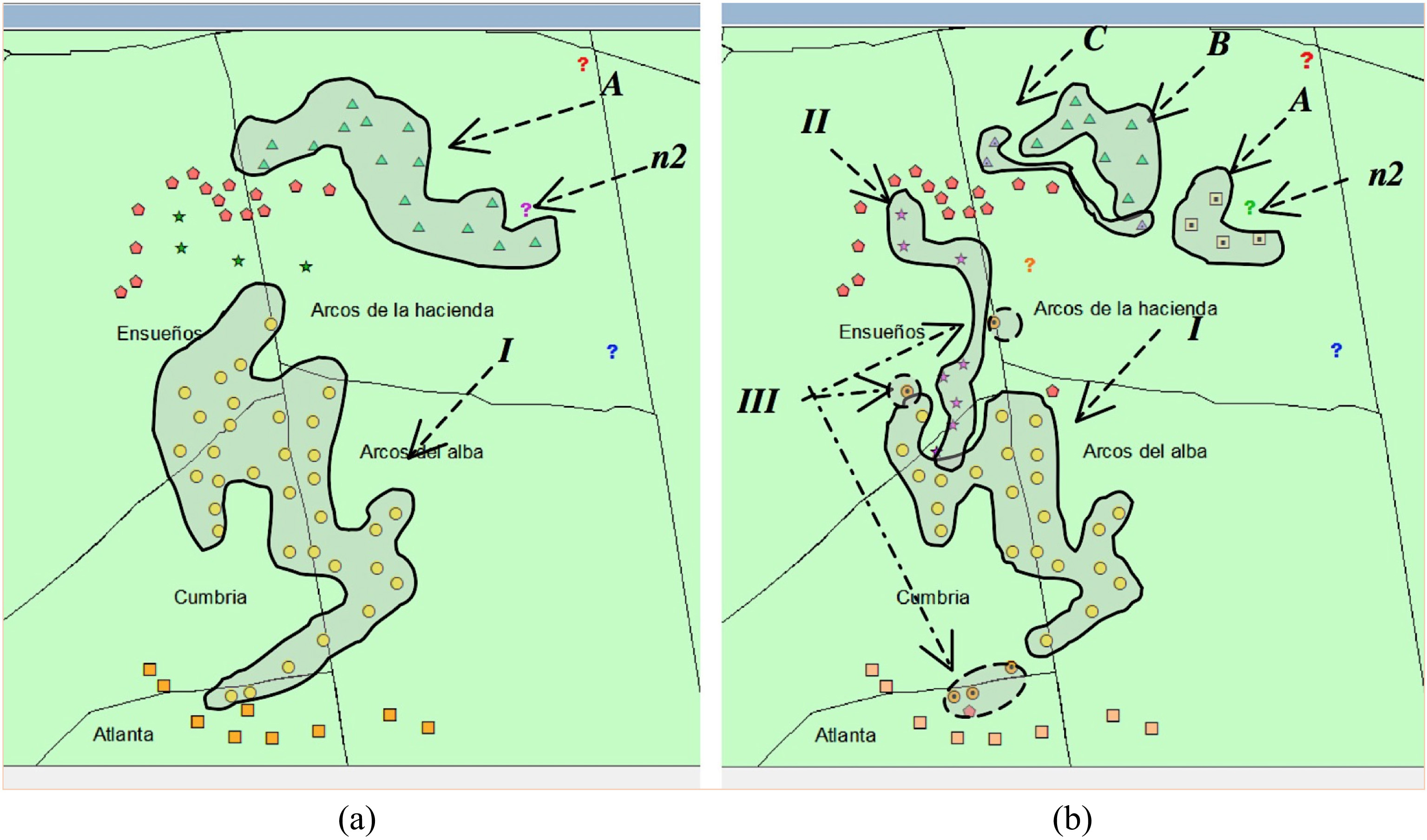

Cluster A (see Fig. 9(a)) represents burglary acts perpetrated with a firearm, while the n2 noise pattern is another burglary crime perpetrated with a “non-specified” weapon. Despite this, not all the patterns in cluster A were perpetrated with a “firearm”. The four triangular patterns surrounding the n2 pattern were committed “without weapons” (see Fig. 9(a)). There is where the Euclidean space similarity function fails, because it groups them in the same cluster given their geographic similarity, although they are not closely related.

Figure 9(b) shows this difference, the noise pattern identified by n2 is the same as the noise pattern identified in Fig. 9(a). Cluster A (Fig. 9(b)) contains the four criminal patterns perpetrated using a firearm, while the patterns that make-up Cluster B were committed without weapons. This result turns out to be very important because, following this path, crimes that were probably perpetrated by the same aggressors can be semantically identified.

In the second experiment we worked with patterns that have a higher level of detail, which means more descriptive features. Also, each component (set of related features) in the crime-patterns, were weighted as follows: 60% space-time, 30% crime-specifics and 10% crime features, due to the fact that some features are more important than others.

This experiment is more related with the work performed by the preventive police, since the family of crimes related to robbery is the one under study. This crime-family is made up by: robbery to passerby, break-in, and auto-parts theft.

The weighting may be obtained through a criminology expert. The objective is to identify trends by taking advantage of the expert’s knowledge in criminology. Figure 6 shows the results achieved.

Table 8

Results of clustering of the “robbery” type of crime data

Cluster	Type of crime	Month	Year
	Robbery to passer-by	July, August & September	2006, 2007 & 2008
	Auto-parts theft	July & September	2007 & 2008
	Break-in	January & April	2008
	Auto-parts theft	February & September	2006 & 2007
? (noise)	Break-in	December	2007

Table 8 shows the results of our last experiment. Of the two residential areas studied in the North areas, the one containing a higher amount of crimes from the robbery family is the Santa Barbara residential area, which belongs to the sector with the same name. Besides, we found that those months of the year with the highest incidence of crime are July and September, so it is necessary to undertake programs and campaigns in such sector, and in that season of the year have prevention programs and campaigns to fight this type of crime.

5.3 Route patrolling results

In this section, we present results of three selected cases with MMAS for solving patrolling routes optimization problems as described in previous paragraphs. After several tests, we found the optimal parameters shown in Table 9. We compared our results against a random walk baseline, which consists basically on using the algorithm shown in Fig. 9 (see Section 4.2) without using Eqs 1 and 2, i.e., using a plain random roulette with equal probabilities, and not using pheromones at all.

Table 9
Parameters used in the MMAS algorithm

Alert	Start	End	Ant colony MMAS			Random walk baseline
#	point	point	Cost	Time	Optimal?	Cost	Time	Optimal?
1	1	31	716	23	Yes	819	32	No
2	1	109	674	35	Yes	674	35	Yes
2	1	105	780	35	Yes	1432	43	No
4	1	89	1197	37	Yes	1781	57	No
5	1	64	1964	96	Yes	–	–	N/A

Table 10

Results obtained from experiment A

5.3.1 Goal A: Target route optimization

The goal of this experiment is to optimize routes that were created as a preventive perimeter given an alert call in a point or specific street. For this purpose, 5 points in the map’s neighborhood were randomly selected, as well as a common starting point. See Fig. 12 and Table 10.

Figure 10.

Clusters identified with ST-DBSCAN with a space similarity function based on sector division (Northern area).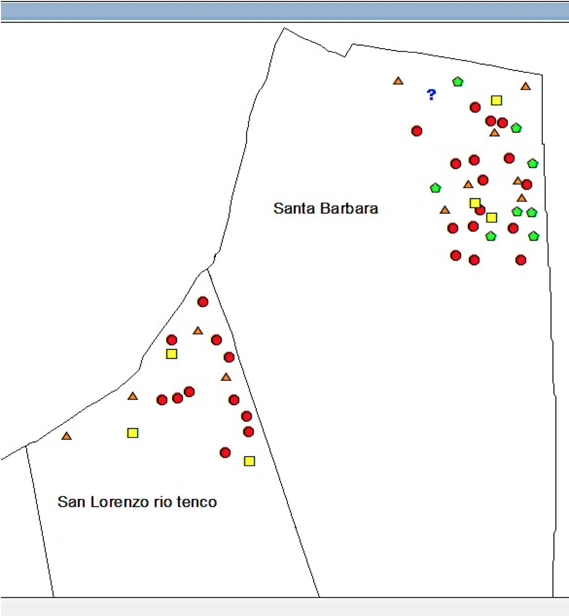

We can see in all cases that the optimal route was automatically found by the ant colony algorithm, while the random walk algorithm did not converge to the optimal solution after the same number of iterations (50), except for Alert 2. For Alerts 1 to 4 the random walk algorithm obtained a route, but for Alert 5 the maximum number of iterations was reached without finding a route to the target node.

5.3.2 Goal B: Route optimization

The goal of this experiment is to find optimal routes for patrolling a small set of nearby streets in a neighborhood. This kind of routes is generally assigned to individual patrols.

For this experiment, three different surveillance areas were selected, each one with 6 nearby points, located randomly in the studied neighborhood, as well as a common point, see Fig. 12. It is important to note that the selected areas were managed independently, and that this experiment aims to illustrate the optimal route from a specific point to a particular area, and so, it does not model interaction with other areas. Optimal routes are shown in Table 11. Our Ant Colony algorithm was able to find all optimal routes for this experiment, whereas the random walk baseline found routes for Alerts 2 and 3, but they were not optimal. See Found routes are ready to be implemented in a real patrolling scenario. Routes like these were calculated for all neighborhoods of Cuautitlán Izcalli, always finding optimal routes.

Table 11
Optimal routes for experiment B

#	Start point	Rute points	Route cost	Time	Optimal route
1	1	59-61-73-75-86-88	2,387	66	1-2-3-6-7-12-18-22-27-26-25-31-41-45-49-50-78-77-76-75-74-73-88-87-86-75-74-73-72-67-68-61-60-59
2	1	31-32-33-39-40-45	1,190	148	1-2-3-6-7-12-18-22-27-33-35-39-108-109-38-34-30-27-33-35-36-32-26-25-31-41-45-49-80-79-40
3	1	91-92-93-95-120-122	2,136	62	1-20-29-37-127-126-125-124-123-122-121-120-95-94-93-69-92-91

Figure 11.

Selected alerts in experiment A.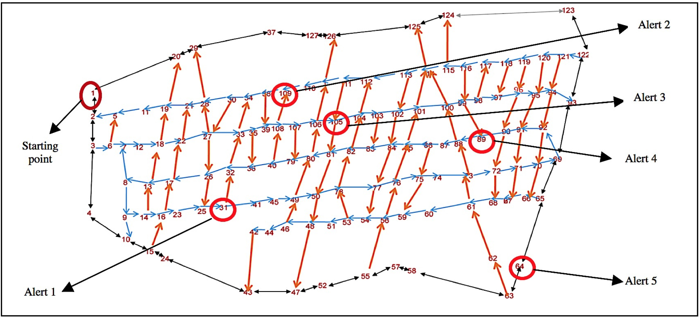

Figure 12.

Selected areas in experiment B from the sample neighborhood.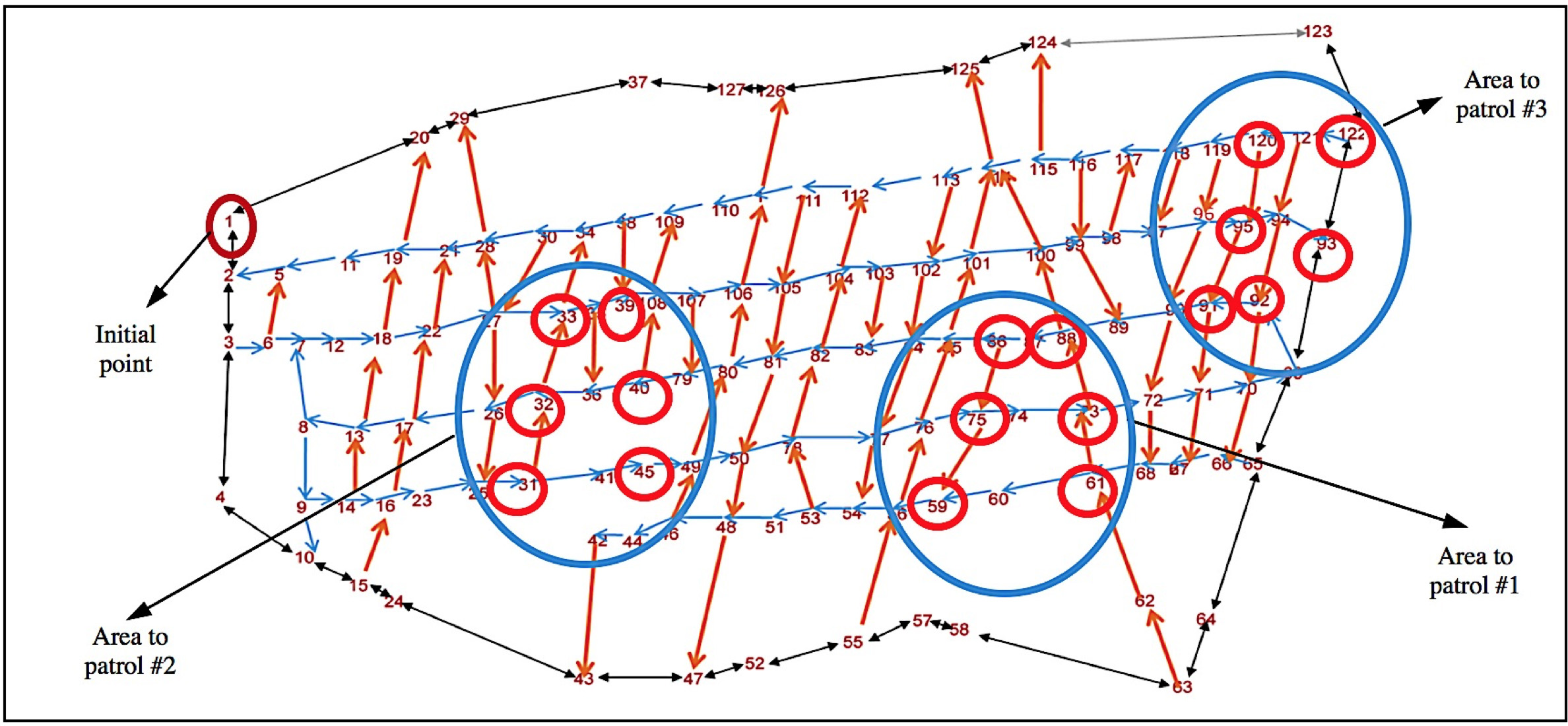

Table 12

MMAS vs. Random walk routes for experiment B

Alert #	Ant colony MMAS			Random walk baseline
	Cost	Time	Optimal?	Cost	Time	Optimal?
1	2,387	66	Yes	–	–	N/A
2	1,190	148	Yes	3,215	217	No
3	2,136	62	Yes	4,384	250	No

Table 13

Optimal routes for experiment C

#	Start point	Rute points	Route cost	Time	Optimal route
1	1	59-61-86-88	4,546	3,421	[l]1-2-3-4-10-15-16-23-25-31-32-33-35-39-108-107-106-105-104-103-102-101-100-99-98-97-96-95-94-93-122-121-120-95-94-93-122-121-120-119-96-90-89-88-87-86-75-74-73-72-68-61-60-59-56-54-53-78-82-81-80-79-40
2		32-33-39-40
3		93-95-120-122
4	1	11-18-21-22	4,126	990	[l]1-2-3-6-7-12-18-22-27-28-21-19-11-5-2-1-20-29-37-127-126-127-37-127-126-125-124-123-122-121-120-119-118-117-116-115-114-113-102-84-77-54-53-51-48-47-52
5		47-48-52-53
6		113-115-124-125

Figure 13.

Areas to be covered by the routes sought in experiment C.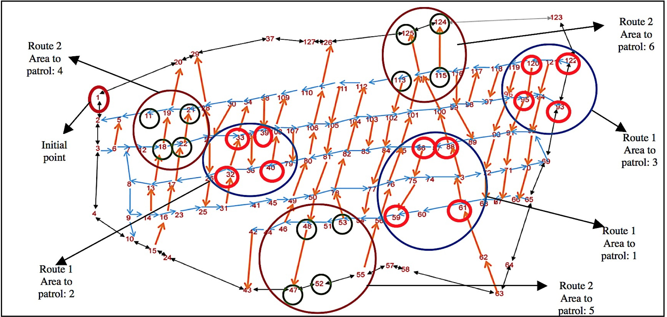

5.3.3 Goal c: Diverse patrolling areas optimization

The goal of this experiment is to find optimal routes for patrolling diverse areas that are distributed throughout the whole neighborhood. For this experiment, the algorithm was executed to find two optimal routes. Each one of them must pass through three different surveillance areas. Each area is integrated with 4 nearby points, randomly selected from the studied neighborhood. All routes depart from a common initial point. See Fig. 13.

All optimal routes shown in Table 13 were found by our Ant Colony Algorithm, while the Random walk algorithm was not able to find a route covering the requested route points within the specified number of iterations. In general, several routes were calculated for all neighborhoods in the municipality of Cuautitlán Izcalli, always finding optimal routes, implying the proposed algorithm is a reliable way of calculating patrolling routes given important points to be covered. These points can be obtained from daily operation of patrolling routes planning sessions.

6. Conclusions and future work

We have presented a framework for forecasting, clustering and patrol routes recommending in order to prevent crime incidents. To our knowledge, this is the first work comprehending a single workflow from raw data of crime events, to patrolling routes recommendation. Each stage of this framework has been validated against methods commonly used by commercial state of the art crime analysis systems, such as Bayesian tendency analysis, Euclidian distance-based clustering, and random walk route generation. In all cases, we were able to provide a performance improvement, as well as other advantages such as obtaining valuable information for describing the criminal scenarios under study by using inductive definitions. We added other flexibilities such as the use of thresholds, which allow us to determine the level of precision we want in the inductive description of each class, and managing several restrictions for covering real patrolling needs.

We performed two analyses: punctual prediction and tendency analysis, which show that it is possible to predict punctually one of four crimes to be perpetrated (crime family, in a specific space and time), and 66% of prediction of the place of crime, despite of the noise of the dataset. The tendency analysis yielded an STRMSE (Spatio-Temporal RMSE), of less than 1.0.

For clustering relevant hotspots, we implemented the ST-DBSCAN algorithm, proposing a space similarity function based on sector division. This generates better results than the standard one based on Euclidean distance, taking the following aspects into account: (1) The semantics adapt better to reality under the context of the type of analysis made and (2) Higher percentage of noise identification contributes to the reduction of elements for the analysis.

Our recommendations on route patrolling were based on ant colony systems, finding that they are efficient and effective for optimizing several kinds of routes. In all cases, we were able to find an optimal route within a limited number of iterations, while the random walk algorithm found an optimal route in only a few cases. For Patrolling Area Optimization, the random walk algorithm was not able to find a patrolling route within the specified number of iterations. These experiments show that computing the probability of transition for an ant based on a pheromone component improves the ability of an exploration algorithm to find a feasible solution in short time.

The problems tackled in our experiments are extendable to cover many problems arising currently in great urban zones of the world. Around 50 iterations were needed to find an optimal route with our method. The compared method was not able to find an optimal route within this number of iterations.

As a future work, there are several paths to explore in this project. First, it is necessary to incorporate other information sources available. Second, it is of the utmost importance to calculate the optimal thresholds for the learning process. A statistical analysis of the data included in the supervision sample would make this task easier, as well as exploring evolutionary techniques [38].

Further experimentation with the baseline algorithm for finding the needed number of iterations to obtain an optimal route (if possible) has been left as future work.

Also, as future work, we plan considering traffic factors affecting patrolling maneuvers, as well as considering other factors impeding free vehicular transit and thus, affect the response time of a patrol.

Footnotes

Acknowledgments

We thank the support of Mexican Government (SNI, SIP-IPN, COFAA-IPN, and BEIFI-IPN), and CONACYT, Red TTL.

References

Agmon

, Multi-robot patrolling and other multi-robot cooperative tasks: An algorithmic approach. Diss, Bar Ilan University, 2009.

Baldwin

and Bottoms

, The urban criminal: A study in Sheffield, London: Tavistock Publications, 1976.

Baskakova

L.V.

and Zhuravlëv

Y.I.

, Recognition algorithm models with representative sets and supporting sets systems (in Russian), Zh Vichislitielnoi Matematiki i Matematicheskoi Fiziki 21(5) (1981), 1264–1275.

Birant

and Kut

, ST-DBSCAN: An algorithm for clustering spatial-temporal data, Data & Knowledge Engineering 60(1) (2007), 208–221.

Block

, STAC hot-spot areas: A statistical tool for law enforcement decisions, in: Crime analysis through computer mapping Block

C.R.

Dabdoub

and Fregly

, eds, Washington, DC: Police Executive Research Forum, 1995, pp. 15–32.

Bongard

M.N.

, Solving geological problems using recognition programs, Journal Soviet Geology C 6 (1963), 147–165.

Calvo

de Oliveira

J.R.

Figueiredo

and Romero

R.A.

, Parametric investigation of a distributed strategy for multiple agents systems applied to cooperative tasks, in: Proceedings of the 29th Annual ACM Symposium on Applied Computing (2014), 207–212.

Capone

D.L.

and Nichols

W.W.

, Jr., Urban structure and criminal mobility, American Behavioral Scientist 20(2) (1976), 199–213.

Carrasco-Ochoa

J.A.

, Representative-sets-based Classifiers, Master’s Thesis, CINVESTAV-IPN, Mexico, 1994.

10.

Cheremesina

E.N.

and Ruiz-Shulcloper

, Cuestiones metodológicas de la aplicación de modelos matemáticos de Reconocimiento de Patrones en zonas del conocimiento poco formalizadas, Revista Ciencias Matemáticas 13(2) (1992), 93–108.

11.

Colorni

A.M.

Dorigo

and Maniezzo

, Distributed optimization by ant colonies, actes de la première conférence européenne sur la vie artificielle, Paris, France, Elsevier Publishing, 1992, pp. 134–142.

12.

Kramer

R.M.

and Tyler

T.R.

, Trust in organizations: Frontiers of theory and research, Sage (1996).

13.

Cressie

, Statistics for spatial data, John Wiley & Sons, 2015.

14.

Dantzig

G.B.

and Ramser

J.H.

, The truck dispatching problem, Management Science 6(1) (1959), 80–91.

15.

De-la-Vega-Doria

L.A.

, Extension to the fuzzy case of the KORA-3 algorithm (in Spanish), Master’s Thesis, CINVESTAV-IPN, Mexico, 1994.

16.

De-la-Vega-Doria

L.A.

Carrasco-Ochoa

J.A.

and Ruiz-Schulcloper

, Fuzzy KORA-Ω algorithm, Proceedings of the 6th European Congress on Intelligent Techniques and Soft Computing, EUFIT, Aachen, Germany (1998), 7–10.

17.

Diukova

E.V.

, On a parametric model of KORA based recognition algorithms (in Russian), Soovshenia po prikladmoi matematiki, Russia, 1998.

18.

Dorigo

and Gambardella

L.M.

, Ant colony system: A cooperative learning approach to the traveling salesman problem, IEEE Transactions on Evolutionary Computation 1(1) (1997), 53–66.

19.

Eck

J.E.

and Maguire

E.R.

, Have changes in policing reduced violent crime? An assessment of the evidence, The Crime Drop in America (2000), 207–228.

20.

Fard

E.S.

Monfaredi

and Nadimi

M.H.

, Application methods of ant colony algorithm, Am J Softw Eng Appl 3(2) (2014), 12–20.

21.

Godoy-Calderón

Calvo

Martínez-Hernández

V.M.

and Moreno-Armendáriz

M.A.

, The CR-Ω+ classification algorithm for spatio-temporal prediction of criminal activity, Journal of Applied Research and Technology 8(1) (2010), 5–23.

22.

Goldfarb

, A new approach to pattern recognition, Progress in Pattern Recognition 2 (1985), 241–402.

23.

Ivaha

Al-Madfai

Higgs

Ware

and Corcoran

, The simple spatial disaggregation approach to spatio-temporal crime forecasting, International Journal of Innovative Computing Information and Control 3(3) (2007), 509–523.

24.

Jefferis

E.S.

, A multi-method exploration of crime hot spots: SaTScan results, National Institute of Justice, Crime Mapping Research Center, (1998).

25.

Jiang

and Claramunt

, A structural approach to the model generalization of an urban street network, GeoInformatica 8(2) (2004), 157–171.

26.

LeBeau

J.L.

, The journey to rape: Geographic distance and the rapist’s method of approaching the victim, Journal of Police Science & Administration (1987).

27.

Levine

, “Hot Spot” analysis using CrimeStat kernel density interpolation, in: Presentation at the Annual Meeting of the Academy of Criminal Justice Sciences (1998), 10–14.

28.

Liu

, ed., Artificial Crime Analysis Systems: Using Computer Simulations and Geographic Information Systems, IGI Global, 2008.

29.

Maniezzo

and Colorni

, The ant system applied to the quadratic assignment problem, IEEE Transactions on Knowledge and Data Engineering 11(5) (1999), 769–778.

30.

Martínez-Trinidad

J.F.

and Guzmán-Arenas

, The logical combinatorial approach to pattern recognition, an overview through selected works, Pattern Recognition 34(4) (2001), 741–751.

31.

Molumby

, Patterns of crime in a university housing project, American Behavioral Scientist 20(2) (1976), 247–259.

32.

Nath

S.V.

, Crime pattern detection using data mining, in: Web Intelligence and Intelligent Agent Technology Workshops, 2006, WI-IAT 2006 Workshops, 2006 IEEE/WIC/ACM International Conference, IEEE (2006), 41–44.

33.

Newman

, Defensible space: Crime prevention through urban design, Ekistics 1 (1973), 325–332.

34.

Portugal

and Rocha

R.P.

, Cooperative multi-robot patrol in an indoor infrastructure, in: Human Behavior Understanding in Networked Sensing, Springer International Publishing (2014), 339–358.

35.

Repetto

T.A.

, Residential crime, Ballinger, Springfield, IL, 1974.

36.

Rossmo

D.K.

, Target patterns of serial murders: A methodological model, American Journal of Criminal Justice 17(2) (1993), 1–21.

37.

Rossmo

D.K.

, Targeting victims: Serial killers and the urban environment, Serial and Mass Murder: Theory, Research and Policy (1996), 133–153.

38.

Sanchez-Diaz

Diaz-Sanchez

Mora-Gonzalez

Piza-Davila

Aguirre-Salado

C.A.

Huerta-Cuellar

Reyes-Cardenas

and Cardenas-Tristan

, An evolutionary algorithm with acceleration operator to generate a subset of typical testors, Pattern Recognition Letters 41 (2014), 34–42.

39.

Scarr

H.A.

Pinsky

J.L.

and Wyatt

D.S.

, Patterns of burglary, Washington, DC: National Institute of Law Enforcement and Criminal Justice, 1973.

40.

Shafahi

and Haghani

, Balanced routing of patrolling vehicles focusing on areas with historical crime, in: Transportation Research Board 94th Annual Meeting 2015 (2015), (No. 15-4387).

41.

Stützle

and Hoos

H.H.

, MAX-MIN ant system, Future Generation Computer Systems 16(8) (2000), 889–914.

42.

Toklu

N.E.

Gambardella