A stacking model for variation prediction of public bicycle traffic flow

Abstract

Public bicycle system can improve the public transport travel efficiency and reduce environmental pollution, which has been deployed in many cities all over the world. However, the bicycle usages become quite skewed and imbalanced in different stations. A system which could recommend the nearest available stations for passengers whether they are looking for a dock or a bike, is of great importance. Monitoring the current number of docks or bikes at each station cannot tackle this problem because it’s too late to recommend the station for passengers to rent or return bikes after the imbalance has occurred. To address this issue, we propose a stacking model for variation prediction of public bicycle traffic flow called SMVP based on the real-world datasets. The stacking model integrates multiple base models which we trained by different combinations of features so that it could get better performance. We adopt a machine learning system called XGBoost [25] to train the models and construct the multiple complex factors which impact the public bicycle traffic flow. The traditional factors, such as temporal, spatial, historical and meteorological factors are taken into consideration. A new clustering factor which considers both the geographical positions and transition patterns of stations is also proposed in this framework and then we use the K-Medoids algorithm [12] to cluster stations into groups by constructing a new different station relation matrix which considers these two factors as the distance between different stations. The performance of SMVP is improved on the datasets of Hangzhou and New York City, especially in terms of Coefficient of Determination improved by 25.58% in Hangzhou, compared with the traditional stacking [5] and single model respectively.

Keywords

Public bicycle traffic flow variation prediction stacking xgboost k-medoids data mining machine learning

1. Introduction

Public bicycle system (also called bicycle-sharing system) is a kind of low-carbon and environment-friendly transportation system, which is vigorously promoted in major cities all over the world, such as Hangzhou, Paris, New York, and other cities. It is designed to solve the “last mile” problem by connecting bus or subway stations to other places. A public bicycle system usually offers bicycles to passengers in a short period of time either for free or costing little charges [20]. The passengers can rent bikes at the stations nearby and return it to the stations near the destination. It is seen as an alternative way of the vehicles for the short-distance trip. It can significantly improve the public transport travel efficiency and reduce environmental pollution. Therefore, public bicycle system is a more and more popular public transportation in cities [10]. As the widely application in recent years, the bicycle usage efficiency has drawn administrators’ attention as the bicycle numbers can be imbalanced at different stations. Some stations have sufficient bikes and no docks while the opposite situation exists as well. The main reason for this problem is the mobility or the one-way use of public bicycles. It means that the passengers rent a bike at one station but return it to another station. Administrators can not schedule the public bicycles in time, which results in the imbalanced bike and dock numbers in each station.

A system which could recommend the nearest available stations for passengers whether they are looking for a dock or a bike, is of great importance nowadays. The ultimate aim of this study is to handle the public bicycle station recommendation problem and get the planning purposes. But the traffic flow prediction is the first step of the recommendation or planning. So, in this paper, we just study the traffic flow prediction of public bicycles traffic flow. The methods of recommendation and the evaluation of planning process will be studied in the future. Indeed, if no prediction method is used in public bicycle system, we also could recommend the stations to passengers based on the real-time monitoring data. But, it may get bad performance because the monitoring the current numbers is too late to recommend the stations for passengers to rent or return bikes after the imbalance has occurred [28]. So, if we can predict the future numbers, passengers could rent or return the bikes to the appropriate stations. The improvement of predicting performance could improve the success rate of renting or returning. So, we try to predict as accurately as possible.

The state of art scalable tree boosting system XGBoost [25] has been widely used by many data scientists to solve the machine learning problems. It has been successfully used in store sale prediction, customer behavior prediction, click through rate prediction, massive online course dropout rate prediction and so on. The success of the system was witnessed in KDD Cup 2015, where XGBoost was used by every winning team in the top-10 [25].

The above observation motivates our work in predicting the public bicycle traffic flow by adopting XGBoost. Other than predicting the bikes, docks, check-in, check-out numbers [28] or passenger flow mentioned in the previous studies. In this paper, we predict the traffic flow variation numbers in a future period. One of the reasons we choose this value as target is that most of the public bicycle systems just store the renting and returning data of the passengers instead of the real-time bike or dock numbers. What’s more, the variation number of bicycles can reflect the number changes at each station immediately. When we recommend the stations to passengers, the dynamically variation values in a future time period can be easily predicted and we can determine whether or not the dynamic changes exceed the threshold we have set before. Combine with the distance between users and stations, we can recommend the best station for the users to help them rent or return bikes successfully. We will verify the proposed model through the datasets of Hangzhou and New York City.

Hangzhou is the first city to set up public bicycle system and it has covered nearly 3 thousand stations, a total of about 60 thousand bicycles. The system produces around 10 millions of record data in a month time. It has already become the largest public bike system in the world. People who are over the age of 16 and under 70 are eligible to rent a bike. We will select the Hangzhou datasets as representative for analysis.

The major contributions of this paper can be concluded as follows:

•
We design a stacking model for variation prediction of public bicycle traffic flow called SMVP. The stacking model integrates multiple base models which we trained by XGBoost [25] based on different combinations of features.
•
A new clustering factor which considers the geographical positions and transition patterns are analyzed as a feature in proposed model. We construct a new different station relation matrix which considers the two factors as the distance between different stations and use the K-Medoids [12] algorithm to cluster stations into groups.
•
The proposed model is verified through datasets including 40 million real-world records of two cities, in which 90% of the datasets are used for training and the rest 10% are used for validation.

The remaining part of the paper is organized as follow. We firstly discuss the related work in Section 2. In Section 3, the variation of traffic flow prediction problem is formulated. In Section 4, we analyze several factors that impact the bike traffic, especially the new clustering factor we proposed and then we introduce the K-Medoids algorithm and construct a station relation matrix. We construct the features based on the analysis and clustering results, introduce XGBoost to train models and design a stacking model for variation prediction (SMVP) in Section 5. The clustering and prediction results are evaluated in Section 6. Finally, we conclude the paper in Section 7.
2. Related work

In recent years, public bicycle has received increasing attention. Because it is significant for promoting environmental travel and enhance the last mile connection to other transit. DeMaio [19] gave an introduction of bicycle-sharing systems in history, impacts, models and future. Etienne et al. [4] studied the statistical model of public bicycle travel based on Velib public bicycle system in French Paris. Midgley [21] analyzed the state-of-the-art and the experience of the public bicycle system in several European public bicycle stations. These are the early studies of public bicycles and give us the concept and working mechanisms of public bicycle systems. Because the usages of public bikes are quite skewed and imbalanced. Pavone et al. [14] developed methods for maximizing the throughput of a mobility-on-demand urban transportation system and introduced a rebalancing policy that minimizes the number of vehicles performing rebalancing trips and this gives vital inspiration to solve the public bicycle load balance problem.

To study the behavior pattern of the public bicycle system can help us to understand the mobility of the public bicycle traffic flow. Froehlich et al. [7] provided a spatiotemporal analysis of 13 weeks of bicycle station usage from Barcelona’s shared bicycling system. Kaltenbrunner et al. [1] provided an analysis of human mobility data in an urban area using the amount of available bikes in the stations of the community bicycle program Bicing in Barcelona. Vogel et al. [23] adopted clustering and validation to analyze the bike usage pattern in Vienna. These studies help us to understand the mobility of public bicycle traffic flow and get the idea of station clustering based on the geographical positions and transition patterns. The reallocation of bikes is very important to compensate the unbalanced bike usage. Contardo et al. [3] and Benchimol et al. [13] presented mathematical formulations to route vehicles to transit the bikes, considering external features, such as the capacity of a vehicle, how unbalanced the distribution of bikes is, etc. Monitoring the current number of docks or bikes at each station is too late to reallocation the bikes after the imbalance has occurred. So the prediction can help to detect the potential imbalance in advance.

There are many studies focus on public bicycle traffic prediction. Borgnat et al. [18] used the dataset of Velov bicycle system to predict the entire traffic in each hour of the day by a combination model. Vogel et al. [23, 22] used the time series analysis to forcast the bike demand in Vienna and Yoon et al. [9] used a modified ARIMA model to predict the available bikes or docks at each station by considering the temporal and spatial factors. We learned the traditional impact influence from this studies. Zheng et al. [28] predicted the traffic flow about chek-in and check-out of the areas on the New York and Washington public bicycle systems from the macro point of view and contribute a clustering algorithm by using K-Means and transition matrix. Zhang et al. [10] used the GBRT and Lasso regression to predict the user behavior and travel time of Chicago public bicycle-sharing system, it was about the microscopic point of view. These studies are focus on predicting the bikes, docks, check-in, check-out numbers or passenger flow. Indeed, there are close internal relationship between these values and the variation traffic flow values which we will predict. Therefore, they provided us the ideas to find the impact factors of public bicycle traffic flow, construct features and train models by machine learning algorithms such as gradient tree boosting.

The researches focus on the gradient boosting methods and ensemble learning methods are also increasing in recent years. The gradient boosting system XGBoost which we adopted in this paper was widely used in many prediction problems recently. Zhang et al. [17] proposed an approach for forecasting passenger boarding choices and public transit passenger flow by using XGBoost. The prediction model was based on mining common user behaviors for semantic trajectories and enriching features using knowledge from geographic and weather data. Wistuba et al. [15] adopted XGBoost to predict the bank card usage for the ECML-PKDD 2016 Discovery Challenge on Bank Card Usage task and achieved better performance on the leaderboard. Horituchi et al. [27] proposed predictive models training by XGBoost and using flight information. The results showed that this regression model predicts the amount of fuel consumption more accurately than flight dispatchers. The stacking methods was first proposed by Wolpert [5] in 1992. Following Wolpert’s stacking methods, Deng et al. [11] constructed many simplified neural network modules further stacked to build a Deep Stacking Network (DSN). Xia et al. [24] obtained the best results in sentiment classification using stacking methods in comparison with other ensemble methods. Li et al. [26] used stacking models with different views of features called Multi-View Stacking Ensemble (MVSE) based on gradient boosting tree to recommend the items for mobile users and they win the first prize of Ali Mobile Recommendation Algorithm Competition in 2015. The implement of stacking models with gradient boosting in other industries had got better performance. Therefore, these studies gave us the idea to adopt XGBoost and train stacking models to get better prediction performance in the field of public bicycle system.

3. Problem formulation

In this section, we will introduce the formulation of the variation of traffic flow prediction problem of public bicycles. The variation of traffic flow prediction problem aims at inferring the variation number of bikes people rent or return at a certain station in a future period of time and they are continuous values. The positive value means the number of people return bikes is higer than renting bikes while the negative value is the opposite. We regard this problem as a regression problem.

The variation of traffic flow prediction can be expressed as, for the sample $i$ in the station $s$ at the time $t$ , we predict the variation numbers $\hat{y}_{i}(s,t)\in\mathbb{R}$ . The initial datasets cannot be trained by machine learning algorithms immediately. We need to extract the corresponding features based on the impact factors from the datasets and they will be expressed as a feature vector $\mathbf{x_{i}}(s,t)\in\mathbb{R}^{m}$ , where $m$ is the dimension of the features. Feature extraction starts from the initial datasets and builds feature intended to be informative and non-redundant, facilitating the subsequent learning and generalization step. According to the datasets including real-world records, we use the actual variation of traffic flow $y_{i}(s,t)\in\mathbb{R}$ as the ground truth.

We use the most of the samples in the datasets as training set $T$ include the ground truth $\{y_{i}(s,t)\}$ , $T$ can be expressed as $T=\{(\mathbf{x_{i}}(s,t),y_{i}(s,t))\}(|T|=n,\mathbf{x_{i}}(s,t)\in\mathbb{R}^% {m},y_{i}(s,t)\in\mathbb{R})$ , where $n$ is the number of samples. The prediction problem can be express as a regression function $\phi:\mathbb{R}^{m}\rightarrow\mathbb{R}$ , where $\phi$ maps the feature vector to the variation of traffic flow. And then this regression function will be used on the test set and get the prediction results $\hat{y}(s,t)$ . Our goal is to find the regression function $\phi$ .

Figure 1.

Average variation of traffic flow under different weather conditions.

4. Impact factor analysis

To predict the variation of traffic flow in each public bicycle station, we need to identify the factors that have important impacts on the public bicycle traffic. In this section, we will first analyze the relationship between traditional factors such as meteorological, temporal, historical and spatial factors. Then we will study the geographical positions and transition patterns between different stations and consider a new clustering factor which concludes these two factors. Finally, we propose a new clustering method that can divide the stations into groups in order to represent different stations types. The station clustering considers the geographical positions and transition patterns. It is designed to discover the underlying pattern of the traffic variation in a cluster. The clustering factor is deriving from the existing factors such as the longitude, latitude and the transition patterns of the userâ€™s historical datasets. In Section 5.1, These impact factors will be constructed as features in the following section.

We use over 20 million historical renting and return records of passengers dataset of Hangzhou public bicycle system, which ranges from April 8th to June 22th in 2016. The meteorological dataset of Hangzhou City corresponding to that time periods from China Meteorological Administration website [29] were collected as well. The detail description of the two datasets will be introduced in Section 6.

4.1 Traditional factors

4.1.1 Meteorological factors

Meteorological factors are important factors affecting public traffic, public bicycle is no exception [28]. Therefore, analyzing the impact of different meteorological factors on the variation of traffic flow of public bicycle is necessary. Firstly, we sum the variation of traffic flow of all the records on each day and then take the average of the total numbers grouped by different kinds of weather condition, wind direction, Beaufort wind force scale and temperature and draw them on 4 figures. Then we will analyze the relationships between the variation of traffic flow and different kinds of meteorological factors.

Figure 2.

Average variation of traffic flow under different wind directions.

Figure 3.

Average variation of traffic flow under different wind force scale.

Figure 1 shows the relationship between weather condition and the variation of traffic flow. We can see that the values are lower in sunny, cloudy and overcast weather conditions, which means that people rent more bikes at most of the stations. However, when the day is raining(include shower, light rain, moderate rain and heavy rain), the variation values are higher while the bike renting amount is less than the other weather condition. In Fig. 2, the variation values are slightly different, but there are no significant relationship between the wind direction and the variation of traffic flow. So the wind direction factor will not be considered being used for the prediction. Compared to the wind direction, as we can see in Fig. 3, the impact of Beaufort wind force scale is greater. In Hangzhou, the Beaufort wind force scale is usually in 3–5 (12–38 km/h). Most of people would like to rent bikes when the Beaufort wind force scale ranges from 3 to 4 (12–28 km/h). When the speed reaches to 5 (29–38 km/h), the bike renting amount decrease significantly. Therefore, Beaufort wind force scale is an important factor. In Fig. 4, with the change of temperature (the unit is Celsius ( ${}^{\circ}$ C)), the renting amount of public bicycle increase firstly and then decrease. When the temperature is less than 18 ${}^{\circ}$ C or more than 22 ${}^{\circ}$ C, the variation values are higher while the renting amount is smaller. Because the temperature is not suitable for passengers to ride bikes. In summary, meteorological factors have greater impact on public bicycle travel, especially the weather condition, Beaufort wind force scale and temperature.

Figure 4.

Relationship between average temperature and the variation of traffic flow.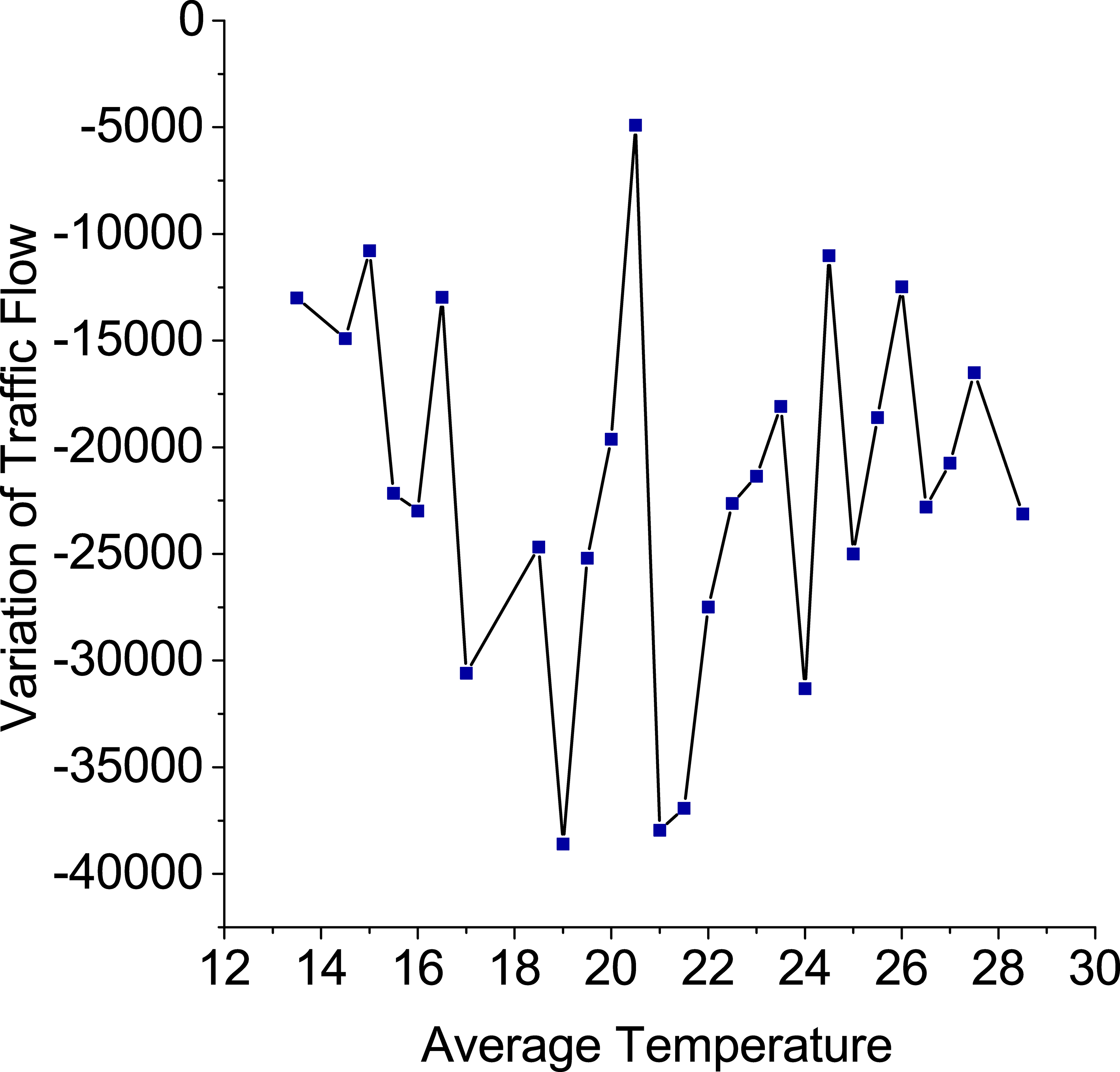

In addition, we can obviously see that the average variation always seems to be negative over the considered period (a day from 6 a.m. to 22 p.m.), which appears to indicate that more bikes are rented than returned every day. This is because that there are many staff of public bicycle company help to maintain some stations which passengers always return the bike to these stations (such as stations near the West Lake). So, these bikes are returned by the staff instead of normal ways and these behaviors are not recorded by the system. There are nearly 300 thousands of passengers using bikes and 30 to 40 thousands of these kinds of abnormal records each day. This also reflects the serious imbalance in different stations.

4.1.2 Temporal factors

The temporal factor plays an important role in our problem. In order to view data from the overall focus on the daily usage of the public bicycle, we count the total volume of the number of passengers and the variation of traffic flow of all the public bicycle stations every day. The total volume of the number of passengers means that we calculated the total volume of passengers renting or returning bikes at all the stations each day. First of all, as is shown in Fig. 5a and b, the distribution of passengers and variation of traffic flow in general are relatively stable. There are certain periodic regularity that less people rent public bikes on weekends, holidays and more people rent bikes in working days. Secondly, compared with Fig. 5a and b, we can see that the variation of traffic flow decrease when the number of passengers increase. These two values are in opposite trend. We can also infer that the number of bicycles that rent by passengers are larger than return because most of the values are negative. Because some passengers did not return the bikes on the same day and return later. Finally, it should be noted that there is an abnormal data on May 23, the total number of passengers on that day is just 6 because of the exception taken by the public bicycle system. By the above analysis, we can see that the month and day are important factors which can reflect the variation of traffic flow.

Figure 5.

Statistics of the number of passenger and the relative variation of traffic flow of bicycles on each day. (a): The number of passengers; (b): The variation of traffic flow of bicycles.

Figure 6.

Periodic analysis. (a): variation of traffic flow on each day in a week; (b): variation of traffic flow on each hour in a day.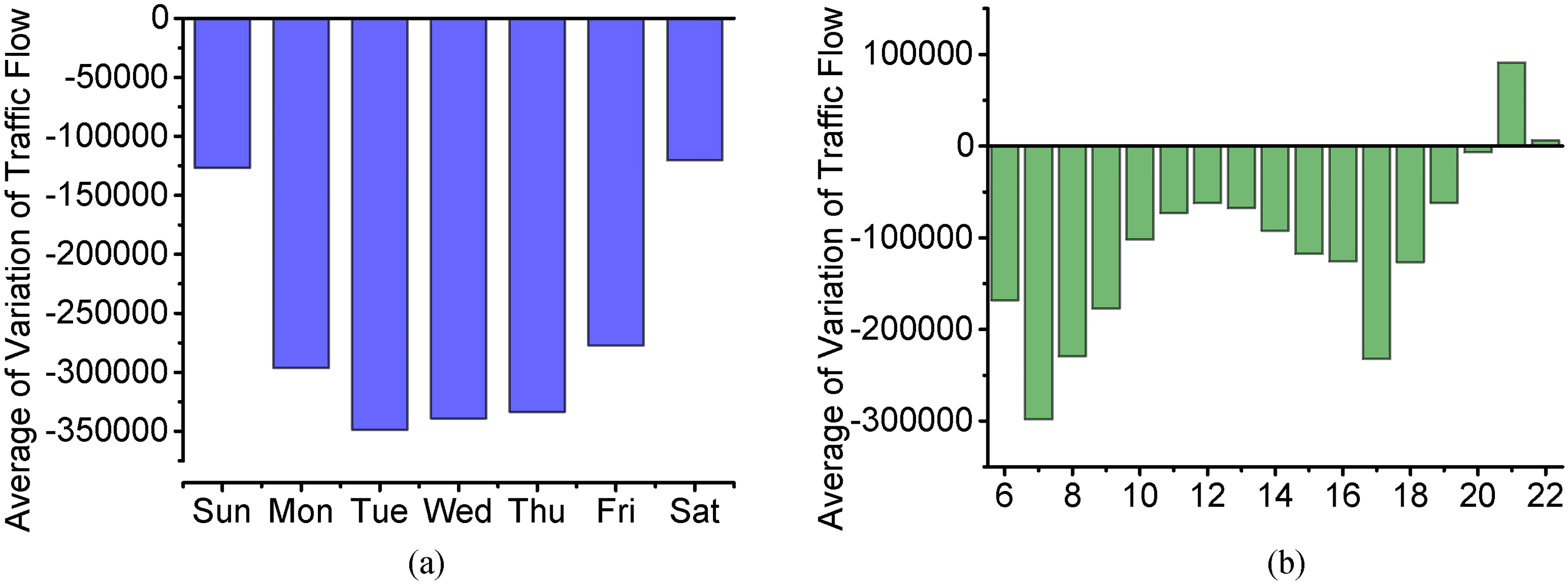

In Fig. 12a, we calculate the sum of variation of traffic flow on each day in a week, which can be analyzed, the renting amount is higher from Monday to Friday and lower on the weekends. In combination with the Fig. 5b, we can see that there is a regular pattern of periodic variation in each week. In Fig. 12b, we calculate the sum of the variation of traffic flow on each hour in a day. It is clear to see that in the early peak (about 7 a.m.) and evening peak (about 17 p.m.), there are more people rent bikes. At noon (about 12 a.m.) and night (about 20 p.m.), less people rent bikes. It is worth noting that lots of people return bike at about 22 p.m. Because people must promptly return the bike on that day, otherwise it will cost more fee. Therefore, it can be found that the week, hour and minute are important factors which can reflect the variation of traffic flow. In Fig. 7, we calculate the average variation of traffic flow grouped by holiday, workday and weekend. It can be seen that compared with the weekend, there are more passenger rent bicycles on holiday. But compared to workday, the number of renting bicycles is smaller. It can be learned that the holiday is also one of the factors affecting public bicycle traffic and the workday also influent the traffic. It is not completely consistent with the workday from Monday to Friday because of the leave reason. Citizens may need to work on the weekend or leave on workday. So if people actually on work is also an important factor.

Figure 7.

Variation of traffic flow in different kind of days.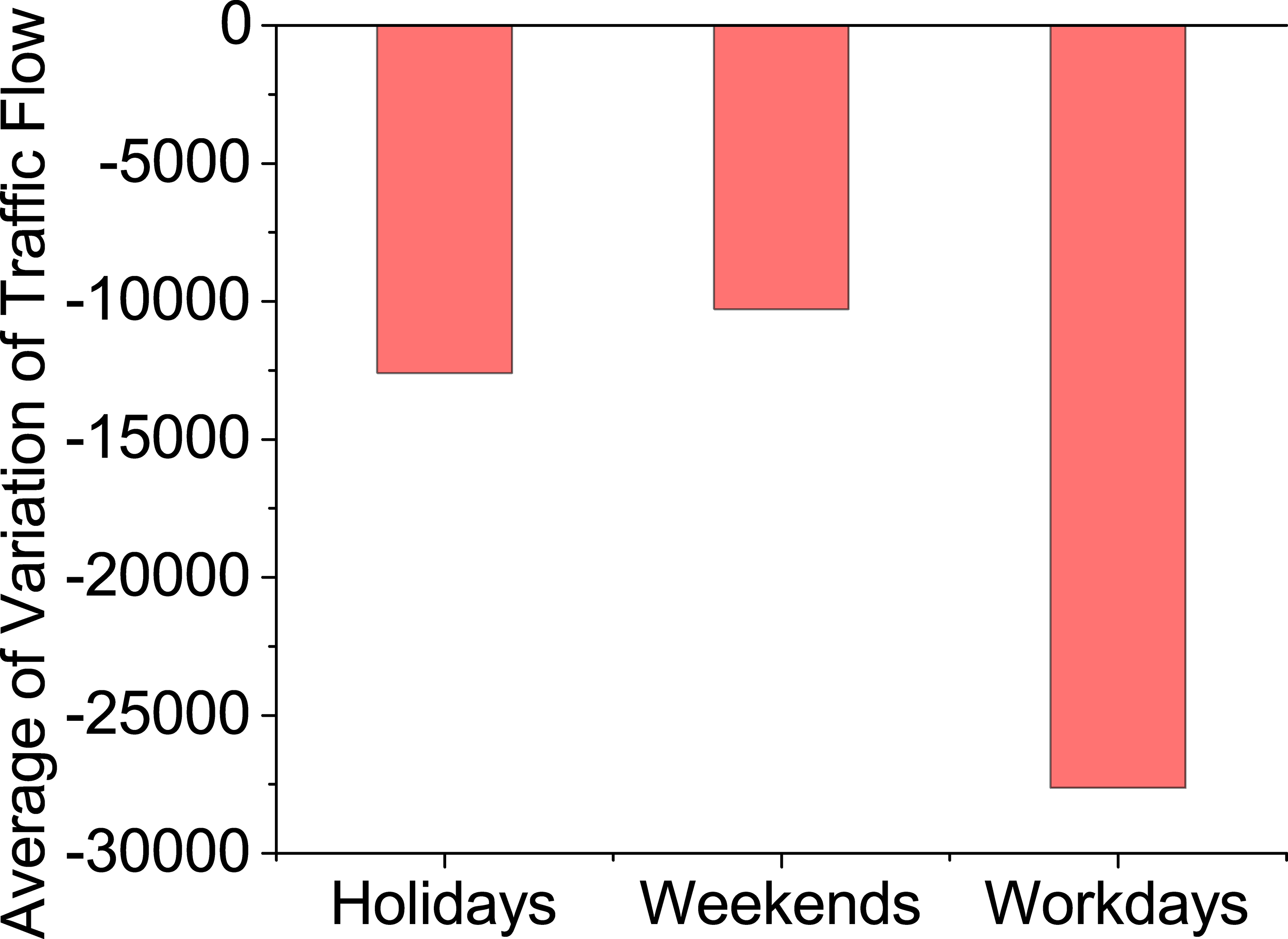

Figure 8.

Variation of traffic flow in different historical days.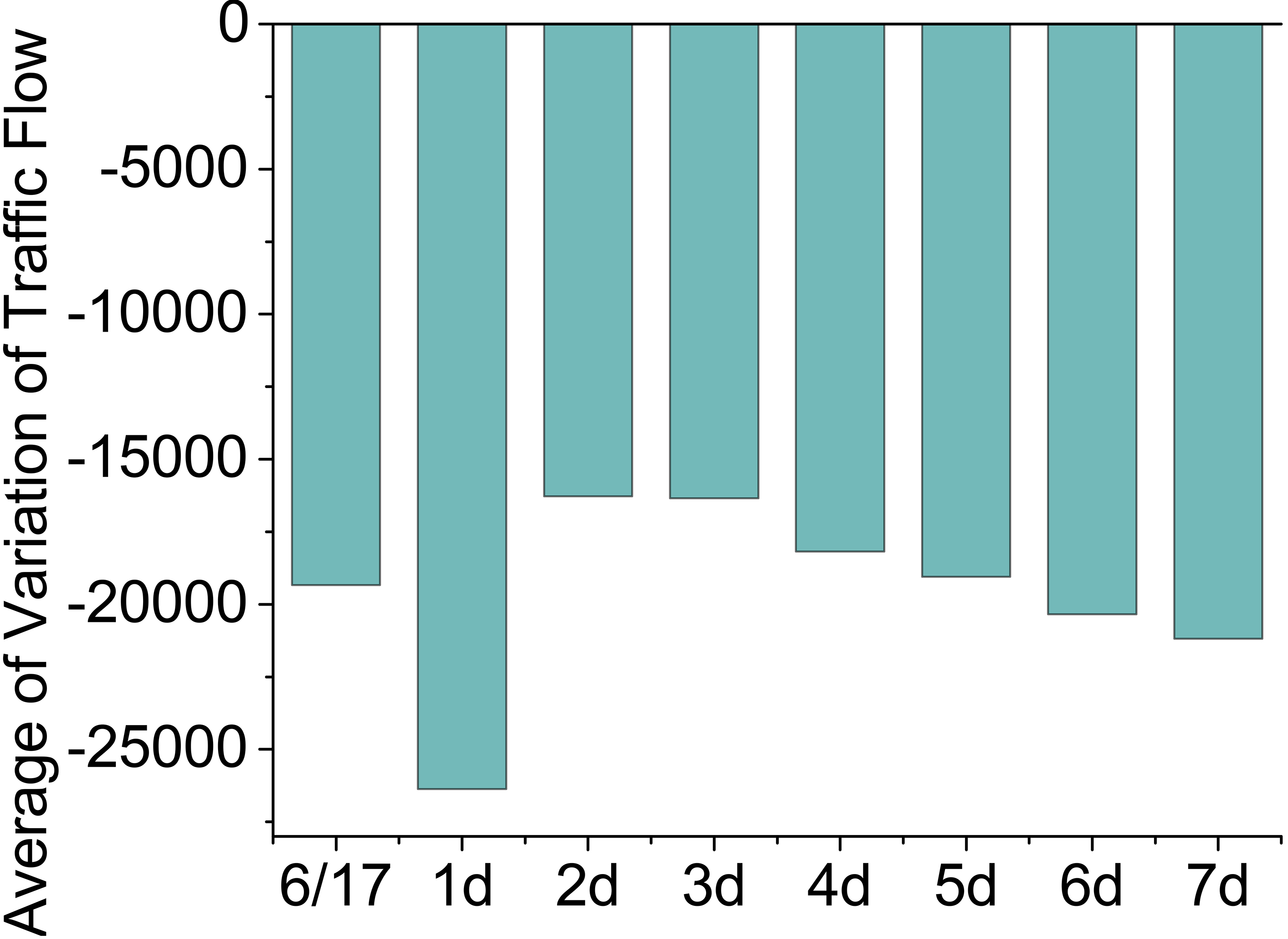

4.1.3 Historical factors

The historical data is also helpful to the public bicycle traffic prediction [28]. In Fig. 8, we chose June 17 as an example and calculate the average variation of traffic flow from several days ago before that day. It can be seen that compared with the June 17, when the day is earlier than this day, the average values are nearly approached to the value of this day. Because we take the mean values of several days, it will be more stable and regular. It’s the same to the several weeks or several months ago. To a certain extent, the historical values reflect the average numbers of several days ago at each station. It can help to estimate the future prediction values. So the historical values are verified through our dataset as an important factors.

4.1.4 Spatial factors

In order to see the spatial distribution of Hangzhou public bicycle on the whole, we plotted each station on the map by the location in Fig. 9, we can clearly see that most of the stations are in urban traffic intensive areas, there are some stations located in the scenic areas such as West Lake, Lingyin Temple and the nearby and some stations distributed near the suburban location. So we choose the station ID as a factor that can distinguish different stations. The latitude and longitude values also reflect the spatial characteristics of the stations, and they will also be used in the following new clustering factor we proposed in this paper.

Figure 9.

The spatial distribution of Hangzhou public bicycle stations.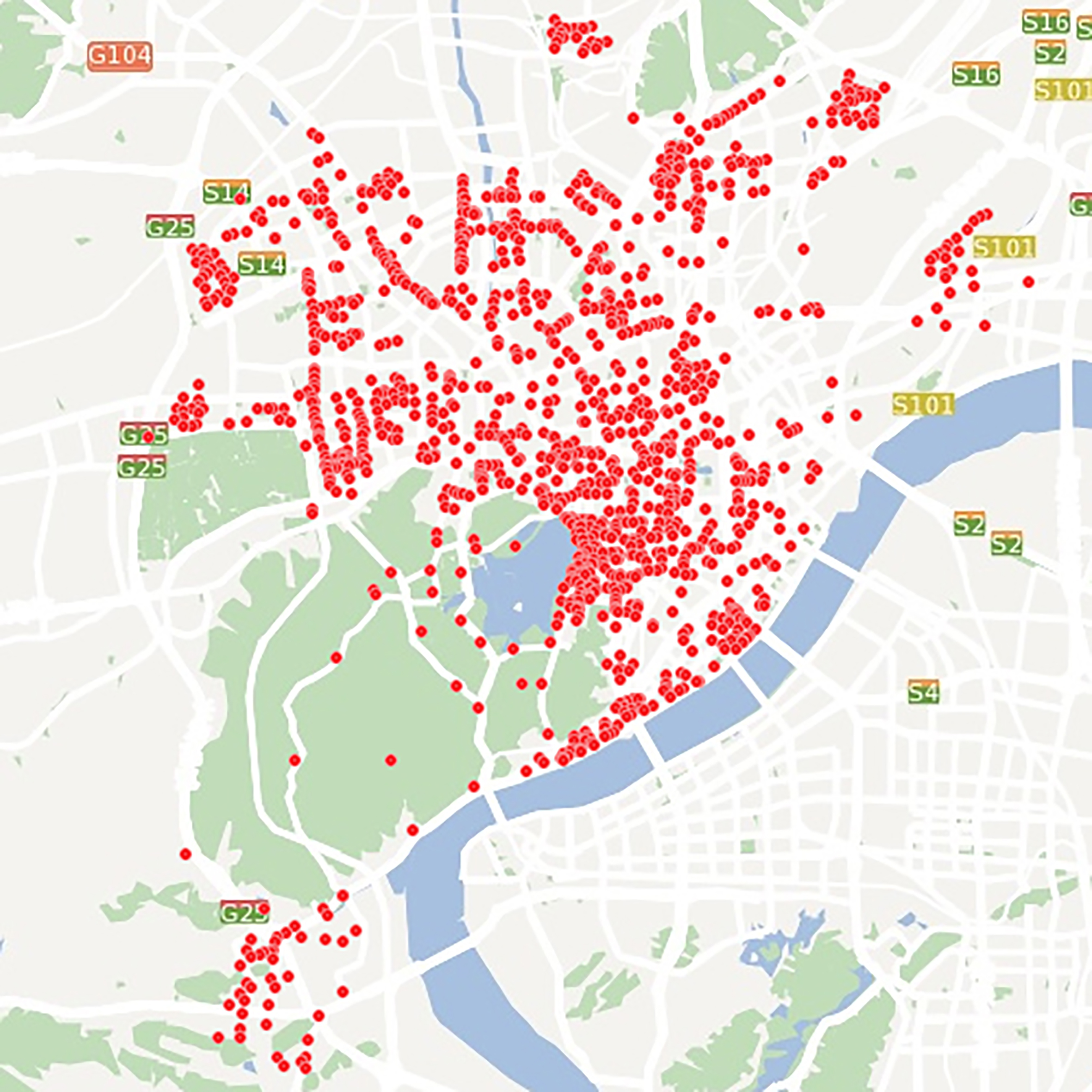

4.2 Clustering factor

The traditional spatial factors just consider the geographical positions of the stations, in this section, we will introduce a new clustering factor that considers both the geographical positions and the transition patterns between the stations. We will analyze the relationship between different stations and use the K-Medoids algorithm to cluster stations into groups by constructing a station relation matrix which considers these two factors as the distance between different stations.

4.2.1 Relationship between stations

There are different regularities in different stations, but stations at the same area may have similar regularities, such as the stations at shopping district, community, attractions area, etc. So we consider clustering the stations into different groups. We need to discuss the relationship between stations firstly. There are two kinds of relation between the stations. One is the geographical position and another is the transition pattern between the stations. If users rent a bike at station A and then return the bike at station B, there will be a transition pattern between stations A and B. In order to find the spatial distribution of relationship between the nearby stations, we draw the station number 1001 and the other stations that are close to it by transition patterns on the map. Station 1001 is the famous spots in West Lake scenic. As we can see in Fig. 10, the stations that have geographical relationship with the station 1001 means that they are close to it on distance and they are marked by blue points. The transition pattern means that the stations that are related with station 1001 by the renting and return behaviors of passengers and they are marked by purple points. The brown points marked in the Fig. 10 are the stations that both have geographical relationship and transition pattern with station 1001. From the points of the map, we can see that the stations close to station 1001 are all belong to the West Lake area. So we consider clustering these stations together by the two aspects and discovering the underlying pattern of the traffic variation in a cluster by the machine learning model. This factor will be transformed as a feature and validated in the experiment section.

Figure 10.

The nearest stations linear station 1001.

4.2.2 Station clustering

In the above section, we have studied the traditional spatial distribution and the relationship between different public bike stations. The station clustering considers the geographical positions and transition patterns. It is designed to discover the underlying pattern of the traffic variation in a cluster. The K-Medoids algorithm is a clustering algorithm related to the Kmeans algorithm [6] and the medoid shift algorithm [2]. K-Means and K-Medoids both set points into several classes, trying to reduce the distance between classes. However, compared with the K-Means, K-Medoids choose the data point as the clustering center instead of the mean point. In each iteration, the algorithm calculates the distance between the different points to the cluster data point.

The most common way of K-Medoids is Partitioning Around Medoids (PAM) Algorithm [16]. It uses a greedy search method to find the optimal result, but it’s much faster than exhaustive search method. The execution procedure of PAM Algorithm used to cluster the station is as follows. The cost means the sum of distances of stations to their medoid.

Station Clustering by PAM AlgorithmInput: $K$ , the number of station clusters Initialize: select $K$ of the $n$ stations as the medoids. Associate each station to the closest medoid. the cost decreases: each medoid $m$ , each non-medoid station $o$ : Swap $m$ and $o$ , recompute the cost. the total cost increased: undo the swap.

Output: station clustering results, clustering medoid

4.2.3 Station relation matrix

When calculate the medoid stations $m$ and non-medoid stations $o$ in the K-Medoids algorithm, it could directly read the matrix concludes the distance between different stations. This matrix could have been calculated in advance to save time. We need to calculate the distance between different stations concludes the geographical relationship and the transition pattern. So we construct a new matrix called station relation matrix, as is shown in Eq. (1). The matrix is a $n\times n$ matrix where $s_{i,j}$ indicates the distance between station $i$ and station $j$ . The higher the value, the longer the distance. When $i=j$ , it means they are the same station so that the distance is 0.

$\displaystyle\begin{bmatrix}0&s_{1,2}&\cdots&s_{1,n}\\ s_{2,1}&0&\cdots&s_{2,n}\\ \vdots&\vdots&\ddots&\vdots\\ s_{n,1}&s_{n,2}&\cdots&0\end{bmatrix}$ (1)

$s_{i,j}$ is composed by the geographical relationship and the transition patterns. To calculate the geographical relationship between the stations, we use the haversine formula which is shown in Eq. (2). The haversine formula is an equation important in navigation, giving great-circle distances between two points on a sphere from their longitude and latitude. It is a special case of a more general formula in spherical trigonometry, the law of haversines, relating the sides and angles of spherical triangles. So we use this formula to calculate the geographical distance between two stations.

$\displaystyle\begin{split}\displaystyle h_{i,j}&\displaystyle=\textit{sin}^{2}% (\Delta lat)+\textit{cos}(\textit{lat}_{i})\textit{cos}(\textit{lat}_{j})+% \textit{sin}^{2}(\Delta\textit{lng})\\ \displaystyle d_{i,j}&\displaystyle=2\cdot R\cdot\textit{arcsin}(\sqrt{h_{i,j}% })\end{split}$ (2)

Where $(\textit{lng}_{i},\textit{lat}_{i})$ and $(\textit{lng}_{j},\textit{lat}_{j})$ are the latitude and longitude in radians of the two stations. lng is longitude and lat is latitude. These values need to be converted from degrees to radians by multiplying by $\frac{\pi}{180}$ as usual. Besides, $\Delta\textit{lat}=\frac{\textit{lat}_{i}-\textit{lat}_{j}}{2}$ , $\Delta\textit{lng}=\frac{\textit{lng}_{i}-\textit{lng}_{j}}{2}$ and $R$ is the radius of the Earth which is about 6378137 m.

In order to calculate the transition patterns between two stations, we need to calculate $c_{i,j}$ . It counts the transition patterns of station $i$ to another station $j$ . Then we calculate the $p_{i,j}$ in Eq. (3) which means the transition probability from station $i$ to station $j$ . The higher the value is, the larger the probability is and the closer the relationship is.

$\displaystyle p_{i,j}=\frac{c_{i,j}}{\sum_{j=1}^{n}c_{i,j}}$ (3)

Each element $s_{i,j}$ in the station relation matrix is calculated by the Eq. (10):

$\displaystyle s_{i,j}=d_{i,j}(1-\omega p_{i,j})$ (4)

Where $\omega$ is a parameter used to control the weight of $p_{i,j}$ , the specific value need to be determined according to the data and experimental results. Thus, we get a station relation matrix and it can be used to the K-Medoids algorithm to cluster the stations into groups.

The aim of this paper is to predict the variation traffic flow of the public bicycle. So, we can see the clustering as a feature extraction method to improve the prediction accuracy. Maybe the other techniques could also be used to extract the features. More methods to extract the features can be studied in the future works.

5. Prediction model design

We design the prediction model to predict the variation of traffic flow based on the previous analysis. First, we construct the feature vector by the important factors which we analyzed in Section 4. Then we adopt a new and scalable machine learning system called XGBoost to train the base and stacking models. Finally, we design a stacking model for variation prediction called SMVP based on feature combination by using several base models to improve the prediction accuracy.

5.1 Features construction

Based on the impact factors we have analyzed in Section 4, we transform them into features. These features are divided into five groups, meteorological features, temporal features, historical features, spatial features and clustering feature. We will introduce the construction details below.

5.1.1 Meteorological features

Based on the analysis of the influence of meteorological factors, there are more effects on weather, temperature and Beaufort wind force scale. The wind direction has little impact so we do not use this factor. We construct $x_{1}$ as temperature at daytime, $x_{2}$ as temperature at night (the unit of temperature is Celsius ( ${}^{\circ}$ C)) and $x_{3}$ as Beaufort wind force scale. These features are all continuous values. We construct $x_{4}$ as the weather condition. They are discrete variables such as sunny, rainy and etc. Therefore, we can encode the categorical variables into numerical vector using one-hot encoding. Allocate a categorical length vector such as Eq. (5). This method can help to train models to get better performance.

$\displaystyle x_{ij}=\left\{\begin{array}[]{ll}1,&$if $x_{i}$ is in category $% j\\ 0,&$otherwise$\end{array}\right.$ (5)

5.1.2 Temporal features

According to the temporal factors, we construct features $x_{5}$ as months, $x_{6}$ as day, $x_{7}$ as week, $x_{8}$ as hour and $x_{9}$ as minute (the exact minute is not necessary, so we split the minutes into fixed periods because that different cities may need different time periods). These features are all continuous features. Based on the analysis of the holiday and workday, we construct $x_{10}$ as “is today holiday?” and $x_{11}$ as “is today workday?”. These two features are discrete variables such as $x_{10}=$ 1 or $x_{10}=$ 0.

5.1.3 Historical features

From the regularity between the day and its historical days, there are similar rules. So we construct the same period of time in past several days as features, such as $x_{12}$ as the same period of 1 day before, $x_{13}$ as 2 days, $x_{14}$ as 3 days, $x_{15}$ as 4 days, $x_{16}$ as 5 days, $x_{17}$ as 6 days, $x_{18}$ as 7 days (1 week), $x_{19}$ as 14 days (2 weeks), $x_{20}$ as 21 days (3 weeks) and so on. The more historical days we choose, the more missing values are existing. Because in the beginning of the dataset such as April 1, the one day before this day such as March 31 is out of the data range. So there will be many missing values in the feature vector. However, the XGBoost which we adopt can treat the missing values when training models. This is an important reason why we choose it.

5.1.4 The spatial features

According to the analysis in Section 4, the rules between different stations is different. So we can construct the station ID as $x_{21}$ , the latitude of the station as $x_{22}$ and the longitude as $x_{23}$ for spatial features.

5.1.5 The clustering features

After the analysis and clustering in Section 4, we cluster the stations into different groups by geographical relationship and the transition pattern. The stations in the same clusters have similar regularities. So we use the clustering result and one-hot encode the cluster each station belongs to as features $x_{24}$ .

For the station $i$ , the feature vector is constructed as $\mathbf{x_{i}}=\{x_{1},x_{2},...,x_{24}\}$ . Then we will train the model based on these features.

5.2 Gradient boosting model

Based on the features constructed above, the proposed model $\phi$ has to be trained by machine learning algorithms. In this paper, we adopt a new machine learning system based on Gradient Boosted Tree algorithm called XGBoost proposed by Chen and Guestrin [25].

Gradient Boosted Tree is a kind of ensemble learning method using multiple CART (Classification And Regression Tree). It can get more accurate results than the single regression tree [8]. XGBoost is a scalable gradient boosted tree machine learning system and the source code is provided on the Github. The performance of traditional GBM (Gradient Boosted Machine) is pretty good, but the speed is slower than XGBoost. It also supports sparse data and has the approximate algorithm to find the optimal partition using Weighted Quantile Sketch and parallel distributed training, greatly enhance the performance of the learning model and save more time [25].

Given the $n$ samples, $m$ features training set $T$ which we have defined in Section 3, where $T=\{(\mathbf{x_{i}}(s,t),y_{i}(s,t))\}(|T|=n,\mathbf{x_{i}}(s,t)\in\mathbb{R}^% {m},y_{i}(s,t)\in\mathbb{R})$ (in the following part, we use $\mathbf{x_{i}}$ as $\mathbf{x_{i}}(s,t)$ , $y_{i}$ as $y_{i}(s,t)$ and $\hat{y}_{i}$ as $\hat{y}_{i}(s,t)$ ). XGBoost uses model with $K$ trees to do prediction and $\hat{y}_{i}$ is the $i$ th instance predictive value. Its value is equal to the:

$\displaystyle\hat{y}_{i}=\phi(\mathbf{x_{i}})=\sum_{k=1}^{K}f_{k}(\mathbf{x_{i% }}),f_{k}\in F$ (6)

Where $F=\{f(x)=w_{q(x)}\}(q:\mathbb{R}^{m}\rightarrow T,w\in\mathbb{R}^{T})$ is a tree function space and the number of leaves is $T$ . Each $f_{k}$ is associated to an independent tree structure $q$ and leaf weight $w$ . To learn the function of the set $F$ , we need to minimize the regularized objective function:

$\displaystyle\begin{split}\displaystyle L^{(t)}=\sum_{i}l(\hat{y}_{i},y_{i})+% \sum_{k}\Omega(f_{t})\\ \displaystyle\textit{Where}\quad\Omega(f_{t})=\gamma T+\frac{1}{2}\lambda||w||% ^{2}\end{split}$ (7)

The variation prediction is a regression problem. So, we define the objective function as a square loss function like Eq. (8) shows.

$\displaystyle l(\hat{y}_{i},y_{i})=(y_{i}-\hat{y}_{i})^{2}$ (8)

After the training process, the XGBoost could get several best tree structures and the prediction results are ensembled by these trees on the training set. Then these tree structures ensemble as the prediction model $\phi$ . It can predict in the test set and output the prediction results.

5.3 Stacking Model for Variation Prediction

The stacking model (also called stacked generalization) is a kind of ensemble learning method [5], which is used to train the model and predict the result by using the prediction results of bases model as features. First, we can use several machine learning algorithms to train the original data, get multiple prediction models and then construct the results of multiple models as features to train an ensemble model. The prediction result of ensemble model is the final result. Usually, the performance of the stacking model is better than that of the single model. The previous studies such as Deng et al. [11] build a Deep Stacking Network (DSN) and get better performance. Li et al. [26] used stacking models with different views of features called Multi-View Stacking Ensemble (MVSE) based on gradient boosting tree to recommend the items for mobile users. Therefore, these studies gave us the idea to adopt XGBoost and train stacking models to get better prediction performance in the field of public bicycle system.

In the previous part, we constructed several different groups of features from different aspects. Each group of features reflects the traffic regularities of public bicycles from a certain point of view. But using one group of these features to train is one-sided and it’s easy to get weak base models so that the performance of stacking model may not be significantly improved. Therefore, in this paper, we design a stacking model for variation prediction based on feature combination called SMVP. We make the diversity between base models as large as possible. This can avoid training weak base models and get better prediction result after using stacking method. The method in detail is as follows.

First of all, we obtained the feature vector of each station $\mathbf{x}_{i}=\{x_{1},x_{2},\ldots,x_{22}\}$ after feature construction. They are divided into several subsets, respectively: meteorological feature subset $\mathbf{m}_{i}=\{x_{1},x_{2},\ldots,x_{4}\}$ , temporal feature subset $\mathbf{t}_{i}=\{x_{5},x_{6},\ldots,x_{11}\}$ , history feature subset $\mathbf{h}_{i}=\{x_{12},x_{13},\ldots,x_{20}\}$ , spatial feature subset $\mathbf{s}_{i}=\{x_{21},x_{22},x_{23}\}$ and station clustering feature subset $\mathbf{c}_{i}=\{x_{24}\}$ .

After that, we set the combination of the above features. Because the spatial and temporal features reflect the station property and time period. They’re too important for prediction so that these two feature subsets are essential in the training model. Then we combine the two feature subsets with the other feature subsets. After this, we put them into XGBoost to train a new stacking model and then use this ensemble model to predict the final results of the test set. The whole processes are as follows.

$\displaystyle\hat{y}_{\textit{ST}_{i}}=\phi_{\textit{ST}}(\{\mathbf{s}_{i},% \mathbf{t}_{i}\})$ $\displaystyle\hat{y}_{\textit{STM}_{i}}=\phi_{\textit{STM}}(\{\mathbf{s}_{i},% \mathbf{t}_{i},\mathbf{m}_{i}\})$ $\displaystyle\hat{y}_{\textit{STH}_{i}}=\phi_{\textit{STH}}(\{\mathbf{s}_{i},% \mathbf{t}_{i},\mathbf{h}_{i}\})$ $\displaystyle\hat{y}_{\textit{STC}_{i}}=\phi_{\textit{STC}}(\{\mathbf{s}_{i},% \mathbf{t}_{i},\mathbf{c}_{i}\})$ (9) $\displaystyle\hat{y}_{\textit{ALL}_{i}}=\phi_{\textit{ALL}}(\{\mathbf{s}_{i},% \mathbf{t}_{i},\mathbf{m}_{i},\mathbf{h}_{i},\mathbf{c}_{i}\})$

Among them, $\hat{y}_{ST_{i}},\hat{y}_{STM_{i}},\hat{y}_{STH_{i}},\hat{y}_{STC_{i}},\hat{y}% _{ST_{i}},\hat{y}_{ALL_{i}}$ are the prediction results of several models trained by XGoost. We construct them as features and splice them with the original features and then train the new combination model $\phi_{\textit{Stacking}}$ to predict the final results $\hat{y}_{i}$ , as shown below:

$\displaystyle\mathbf{st}_{i}=\{\hat{y}_{ST_{i}},\hat{y}_{STM_{i}},\hat{y}_{STH% _{i}},\hat{y}_{STC_{i}},\hat{y}_{ST_{i}},\hat{y}_{ALL_{i}}\}$ (10) $\displaystyle\hat{y}_{i}=\phi_{\textit{Stacking}}({\mathbf{st}_{i},\mathbf{s}_% {i},\mathbf{t}_{i},\mathbf{m}_{i},\mathbf{h}_{i},\mathbf{c}_{i}})$

The SMVP can not only avoid training weak base models and increase the diversity between different base models and improve the performance of ensemble learning, but also dig out the combination regularities from different combinations of features. This method can improve the generalization ability of the prediction model and enhance the accuracy. The structure of the whole process is as shown in Fig. 7.

6. Experiment

6.1 Settings

6.1.1 Datasets

We conduct experiments on four datasets (bike renting data and meteorology data) from Hanzhou in China and New York City in U.S. The details of initial datasets are presented in Table 1.

Table 1
The details of the initial datasets

Data sources	Hangzhou	New York City
Time span	8th Apr–22th Jun	1st Jan–31st Mar
Stations	1300	632
Bikes	44,755	10,186
Records	19,140,180	2,245,988

Hangzhou (HZ) Data: We use near 20 million historical records and 1300 stations (part) in Hangzhou Public Bicycle System which range from 8th April to 22nd June, 2016. The dataset of user’s historical records includes the record ID, bike ID, card ID, check-in station, check-out station, check-in timestamp, check-out timestamp, check-in dock, check-out dock and etc. We also collect the meteorology data of Hangzhou City corresponding to that time span from China Meteorological Administration website, include weather condition, temperature, wind direction, Beaufort wind force scale and other information.

New York City (NYC) Data: We use the data of Citi Bike System [30] in New York City from 1st Janurary to 31st March, 2017. There are over 2 million historical records, near 10 times less than Hangzhou. The data contains: trip duration, start time, stop time, station ID, station name, station latitude, station longitude, bike ID, user type, birth year, gender and so on. And we use the meteorology data corresponding to that time.

The data preprocessing is carried out in the following way. Firstly, we find out the abnormal data in the historical dataset. For example, (1) there are some records that the return time is earlier than renting time; (2) some passengers rent a bike at a station and then return it into the same station in a short time; (3) there are lots of artificial reallocated data in some stations; (4) there contains missing values at some time period, such as 23th May in Hangzhou, due to the exception of the public bicycle system.

To solve these problems, we need to do some work on data cleaning. We cleaned the records which the return time is earlier than the renting time, passengers rent bikes and return bikes at the same station just in 3 minutes. We also delete the artificial reallocated data in some stations because we only study the variation of traffic flow generated by the passenger of the public bicycle. And we do not need to process the missing values because the XGBoost can treat the missing values when training models.

After data cleaning and features construction, we split each city datasets into two parts, the training set and test set. The Hangzhou datasets range from 8th April to 15th June (10 weeks) are used as training set and the test set ranges from 16th June to 22nd June (a week). The New York City datasets ranges from 9th January to 19th March (10 weeks) are used as training set and the test set rages from 20th March to 26th March (also a week).

6.1.2 Comparison baseline for features

In order to see the effect of the features we constructed, we train 4 models by XGBoost and choose $K$ -fold cross validation set to evaluate these models on the training set. In order to maintain consistency of the target, we take $K$ weeks of datasets and divide them into $K$ parts (each part is a full week). Then we take the other $K-1$ parts to train and predict the rest of the part in each fold and take the average of the $K$ -fold results as the final result. Here, we choose $K=10$ and use 4 baselines to compare the performance of different features. And the result will be the average values of $K$ -fold validation:

ST (Spatial & Temporal Features): We use only the spatial and the temporal features to train the models by XGBoost. It’s used to validate the impact of spatial and temporal features.

STH (Spatial & Temporal & Historical Features): We use the spatial, temporal features and the historical features to train the models by XGBoost. It’s used to validate the impact of historical features.

STHM (Spatial & Temporal & Historical & Meteorological Features): We use the spatial, temporal features, historical features and meteorological features to train the models by XGBoost. It’s used to validate the impact of meteorological features.

STHMC (All Features): We use all the features include the clustering feature to train the models by XGBoost. It’s used to validate the impact of clustering feature. This is the new feature we proposed in this paper.

6.1.3 Comparison baseline for models

The previous studies of public bicycle traffic flow prediction are focus on the number of bikes, docks, check-in, check-out or passenger flow. There are no efficient baseline for the variation prediction of public bicycle traffic flow. Therefore, we build several baselines to compare the performance of different methods on test set to validate the effort of SMVP:

HA (Historical Average): We use the historical average variation values which are one week before the target time period as the prediction results. We use the average variation values from May 19th to June 15th as the prediction results of the test set.

SM (Single Models): We use all the features include the new station clustering feature to train a single model by XGBoost. It’s used to be compared with the historical average values in order to validate the effort of the new single model trained by XGBoost which we adopted in this paper.

Figure 11.

Process of Stacking Model for Variation Prediction (SMVP).

TSM (Traditional Stacking Model): We combine the prediction results of XGBoost single model (using all features) and original features as a new feature vector and then train a traditional stacking model. It will be compared with the single model and the SMVP we designed in this paper.

SVMP (Stacking Model for Variation Prediction): We train the SMVP designed in Section 5.3 by using several base models which trained by different kinds of features. It will be used to compare with the other methods to validate the performance.

6.1.4 Evaluation metrics

We use the MAE (Mean Absolute Error), MSE (Mean Square Error), RMSE (Root Mean Square Error) and $R^{2}$ (Coefficient of Determination) to evaluate the performance of the model. The formula is as follows:

$\displaystyle\textit{MAE}=\frac{1}{N}\sum_{i=1}^{N}|y_{i}-\hat{y}_{i}|$ $\displaystyle\textit{MSE}=\frac{1}{N}\sum_{i=1}^{N}(y_{i}-\hat{y}_{i})^{2}$ $\displaystyle\textit{RMSE}=\sqrt{\frac{1}{N}\sum_{i=1}^{N}(y_{i}-\hat{y}_{i})^% {2}}$ (11) $\displaystyle R^{2}=1-\frac{\sum_{i=1}^{N}(y_{i}-\hat{y}_{i})^{2}}{\sum_{i=1}^% {N}(y_{i}-\bar{y}_{i})^{2}}$

Where, $y_{i}$ is the ground-truth, $\hat{y}_{i}$ is the prediction result, $\bar{y}_{i}$ is the mean value of all the ground-truth and $N$ is the number of sample.

6.2 Results

6.2.1 Results of station clustering

In the clustering experiment, we use empirical parameters $K=10,\omega=100$ and the effect is pretty good both on the two cities. The result of clustering is shown in Fig. 12 and the different colors represent the different clusters. The red marker point is the center of clustering. As we can see that the results are basically in accordance with the actual situation of Hangzhou, such as dark brown points represent the West Lake area, light brown points represent the area along the Qiantang River and the gray points represent the Xixi Wetland region and etc. There is similar performance in New York City.

Table 2
The results (average) of different features on $K$ -fold cross validation

Metric	MAE		MSE		RMSE		$R^{2}$
feature	HZ	NYC	HZ	NYC	HZ	NYC	HZ	NYC
ST	1.025	1.651	2.614	8.043	1.699	2.814	0.045	0.322
STH	1.004	1.559	2.443	7.199	1.673	2.661	0.074	0.395
STHM	1.002	1.545	2.434	6.842	1.672	2.596	0.076	0.422
STHMC	0.997	1.541	2.376	6.669	1.669	2.563	0.079	0.436

Figure 12.

Station clustering results. (a): Hangzhou; (b): New York City.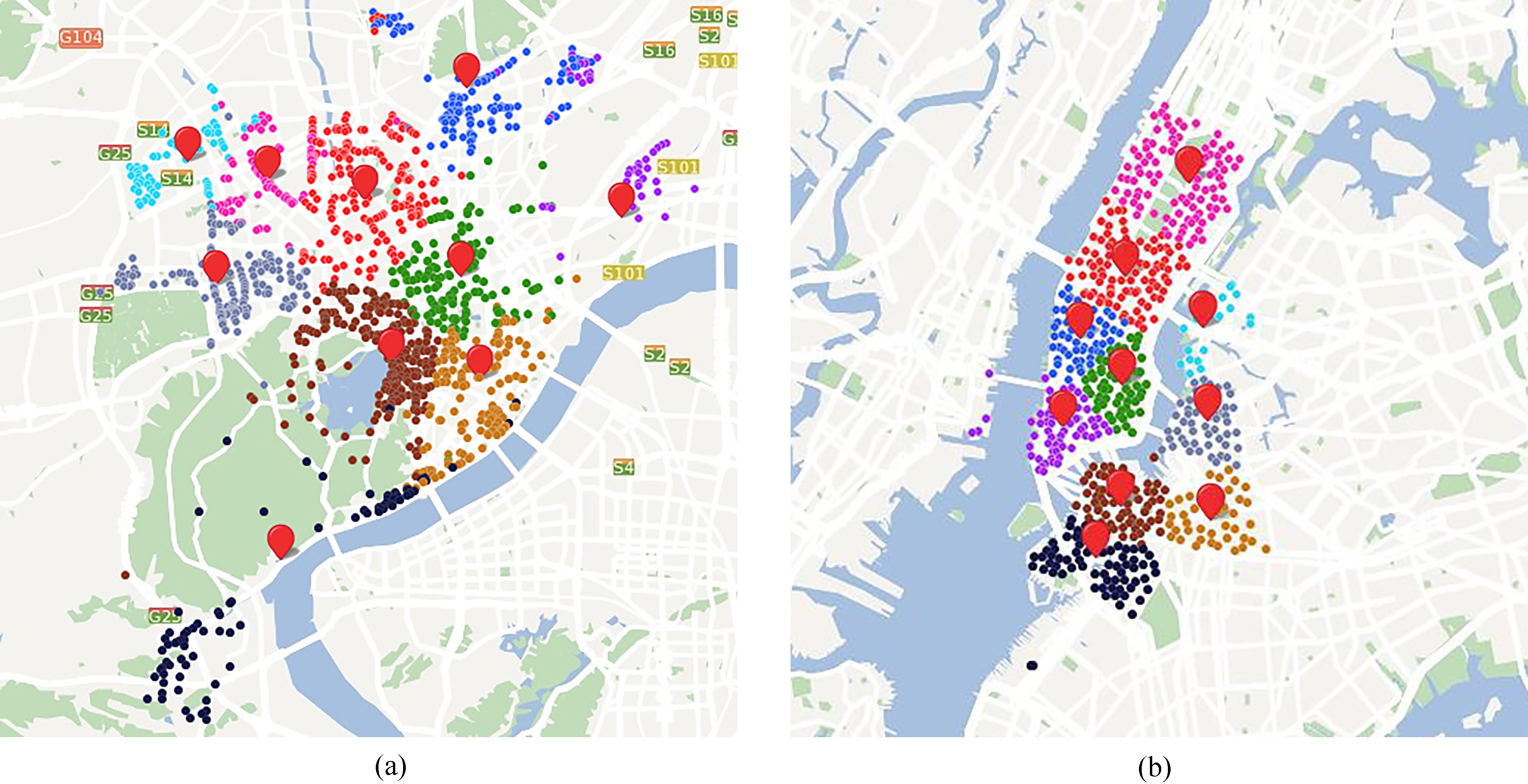

Figure 13.

The effect of different features on $K$ -fold cross validation. (a): MAE; (b): MSE; (c): RMSE; (d): $R^{2}$ .

6.2.2 Results of different features

The results of models based on different features are shown in Table 2 and Fig. 13. We also concentrate on the result of Hangzhou data and the New York City data are similar. We can clearly see the effects of different features. The traditional method which only used the spatial and the temporal features effects the maximum error. The MAE is 1.025, MSE is 2.614, RMSE is 1.699 and $R^{2}$ is about 0.045. After adding the historical features, the error is lower than before. The MAE is about 1.004 and decrease 2.05%, the MSE is about 2.443 and decreased 6.54%, the RMSE is about 1.673 and decreased 1.53% and the $R^{2}$ is about 0.074 and increased 64.44%. So the historical features can enhance the prediction accuracy. When adding the meteorological features, the MAE is about 1.002 and decrease 0.19%, the MSE is about 2.434 and decrease 0.37%, the RMSE is about 1.672 and decrease 0.06% and the $R^{2}$ is about 0.076 and increase 2.7%. It’s a little improvement. That is because the weather, temperature and Beaufort wind force scale in this time period are not so mutable so that the performance is not so obvious, but meteorological features also have impact on the variation of traffic flow prediction. Finally, we add the results of the clustering algorithm as the clustering feature to the models, the error is further reduced. The MAE is about 0.997 which has lower than 1 and decrease 0.49%, the MSE is 2.376 and reduced by 2.38%, the RMSE is 1.669 and reduced by 0.17% and the $R^{2}$ is about 0.079 and increase 3.95%. This proves that the clustering feature proposed in this paper can further improve the accuracy of the prediction model. Because it clustered the similar station together and they have the similar patterns in the variation of traffic flow, so they can help XGBoost divide the samples into different tree leaves and get better model. The results on data from New York City are similar with those on Hangzhou data. This confirms that the clustering feature can get better performance and be used in different public bicycle systems.

Table 3
The results of different models on the test set

Metric	MAE		MSE		RMSE		$R^{2}$
method	HZ	NYC	HZ	NYC	HZ	NYC	HZ	NYC
HA	0.989	1.819	2.614	8.449	1.616	2.906	0.068	0.386
SM	0.906	1.675	2.441	7.893	1.562	2.809	0.083	0.436
TSM	0.898	1.665	2.434	7.697	1.560	2.774	0.086	0.449
SVMP	0.887	1.655	2.375	7.401	1.541	2.721	0.108	0.471

Figure 14.

The effect of different models on the test set. (a): MAE; (b): MSE; (c): RMSE; (d): 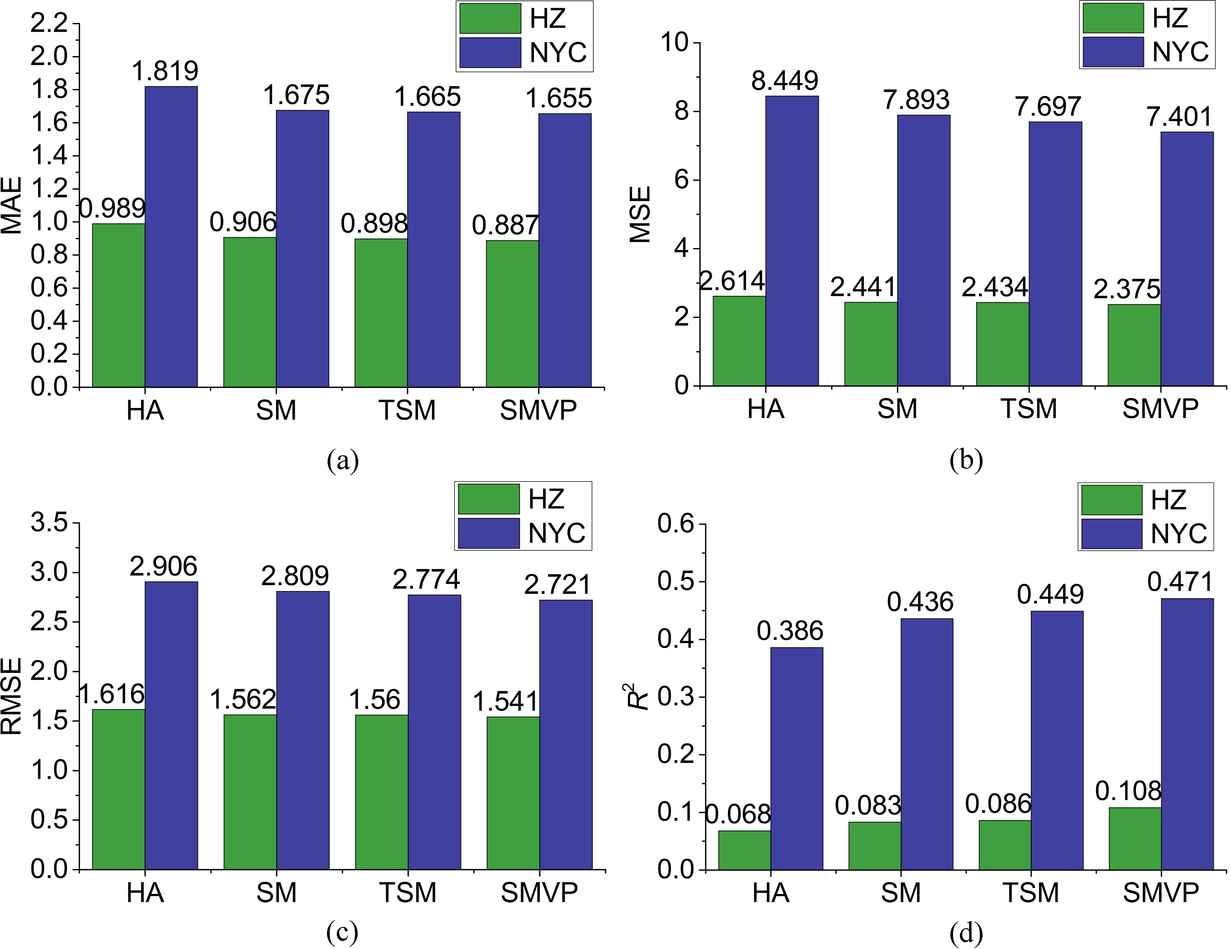$R^{2}$ .

6.2.3 Results of prediction models

We compare the results of different methods and concentrate on the result of Hangzhou data as those of New York City data are similar. From the Table 3 and Fig. 14, we can see that the method of historical average effects the maximum error. The MAE of Hangzhou data is about 0.989, the MSE is about 2.614, the RMSE is about 1.616 and the $R^{2}$ is about 0.068. Compared with historical average, XGBoost single model we train from all the features performs better. The MAE is 0.906 and decrease 8.39%, the MSE is 2.441 and decrease 6.62%, the RMSE is about 1.562 and decrease 3.34% and the $R^{2}$ is 0.083 and increase 22.06%. So the single model trained by XGBoost we adopted have a great effort on the enhance of prediction accuracy. While after using the tradition stacking model, the MAE is 0.898 and decrease 0.88%, the MSE is 2.434 and decrease 0.29%, the RMSE is about 1.560 and decrease 0.13% and the $R^{2}$ is 0.086 and increase 3.61% and it can really improve the accuracy. The SMVP we designed in this paper also have great performance on prediction problem. The MAE is 0.887 and decrease 1.22%, the MSE is 2.375 and decrease 2.42%, the RMSE is about 1.541 and decrease 1.22% and the $R^{2}$ is 0.108 and increase 25.58%. This proves that the models we designed have obviously contributions on the prediction accuracy rising. The results of experiments on data from New York City shown in Table 3 and Fig. 14 are similar with those on Hangzhou data. This confirms that our model is applicable to different public bicycle systems. But the improvement of models based on New York City data is smaller than that on Hangzhou. Because that the data size of Hanzhou is larger than New York City. The larger the size of data, the better the model performs. As the successful application of gradient boosting and stacking in other industries, we verified the proposed algorithm by using two large scale cities datasets to predict the variation traffic flow. The results are shown positive.

7. Conclusion

In this paper, we proposed a stacking model for variation prediction of public bicycle traffic flow at each station called SMVP based on the real-world datasets. We adopted XGBoost [25] to train the models and constructed the multiple complex factors which impact the public bicycle variation of traffic flow. Beside the traditional factors, such as temporal, spatial, historical and meteorological factors were taken into consideration, a new clustering factor which considered the geographical positions and transition patterns of stations was also proposed in this framework. Then we used the K-Medoids algorithm to cluster stations into groups by constructing a new different station relation matrix which considers these two factors as the distance between different stations. We evaluated our models on the datasets of Hangzhou and New York City public bicycle system, the performance of SMVP was improved, especially improved by 25.58% in Hangzhou, compared with the traditional stacking [5] and single model respectively in terms of $R^{2}$ . In the future, we will study the planning process of recommendation and consider to develop a smartphone APP to recommend stations to users by using the advanced ensemble variation of traffic flow prediction model we proposed in this paper.

Footnotes

Acknowledgments

This work is partially supported by the grant from the National Natural Science Foundation of China (No. 61602141 and 61401135), Zhejiang Provincial Public Welfare Technology Application Research Project of China (No. 2015C33067) and the Xinmiao Talent Program of Zhejiang Province (No. 2016R407068).

References

Kaltenbrunner

Meza

Grivolla

Codina

and Banchs

, Urban cycles and mobility patterns: exploring and predicting trends in a bicycle-based public transport system, Pervasive and Mobile Computing 6(4) (2010), 455–466.

Pandey

and Shukla

, Analysis and implementationof k-mean and k-medoids algorithm for large, dataset to increase scalability and efficiency, 2015.

Contardo

Morency

and Rousseau

, Balancing a dynamic public bike-sharing system, CIRRELT, vol. 4, 2012.

Etienne

and Latifa

, Model-based count series clustering for bike sharing system usage mining: a case study with the velib’ system of paris, Acm Transactions on Intelligent Systems & Technology 5(3) (2014), 1–21.

Wolpert

D.H.

, Stacked generalization, Neural networks 5(2) (1992), 241–259.

Hartigan

J.A.

and Wong

M.A.

, Algorithm AS 136: A K-Means Clustering Algorithm, Applied Statistics 28(1) (1979), 100–108.

Froehlich

Neumann

and Oliver

, Sensing and Predicting the Pulse of the City through Shared Bicycling, Proceedings of the International Joint Conference on Artificial Intelligence, IJCAI 2009, 2009, Vol. 38, pp. 1420–1426.

Friedman

J.H.

, Greedy function approximation: a gradient boosting machine, Annals of Statistics 29(5) (2000), 1189–1232.

Yoon

J.W.

Pinelli

and Calabrese

, Cityride: A Predictive Bike Sharing Journey Advisor, IEEE, International Conference on Mobile Data Management, 2012, pp. 306–311.

10.

Zhang

Pan

and Li

, Bicycle-Sharing System Analysis and Trip Prediction, International Conference on Mobile Data Management, MDM’16, 2016.

11.

Deng

and Platt

, Scalable stacking and learning for building deep architectures, IEEE International Conference on Acoustics, Speech and Signal Processing 22 (2012), 2133–2136.

12.

Kaufmann

and Rousseeuw

P.J.

, Clustering by Means of Medoids, Statistical Data Analysis Based on the L1-norm and Related Methods, North-Holland, 1987, pp. 405–416.

13.

Benchimol

Chappert

Taille

A.D.L.

and Laroche

, F Meunier, and Robinet. Balancing the stations of a self service “bike hire” system, RAIRO-Operations Research 45(1) (2011), 37–61.

14.

Pavone

Smith

Frazzoli

and Rus

, Load Balancing for Mobility-on-Demand Systems, Robotics: Science and Systems Vii, University of Southern California, (Vol. 31, pp. 249–256). MIT Press, 2012.

15.

Wistuba

Duongtrung

Schilling

and Schmidtthieme

, Bank card usage prediction exploiting geolocation information, 2016.

16.

Laan

M.V.

Pollard

and Bryan

, A new partitioning around medoids algorithm, Journal of Statistical Computation and Simulation 73(73) (2003), 575–584.

17.

Zhang

Chen

and Chen

, Forecasting public transit use by crowdsensing and semantic trajectory mining: case studies, ISPRS International Journal of Geo-Information 5(10) (2016), 180.

18.

Borgant

Abry

Flandrin

Robardet

Rouquier

and Fleury

, Shared bicycles in a city: a signal processing and data analysis perspective, Advances in Complex Systems 14(3) (2011), 415–438.

19.

Demaio

, Bike-sharing: history, impacts, models of provision, and future, Journal of Public Transportation 12(4) (2009).

20.

Midgley

, Bicycle-Sharing Schemes: Enhancing Sustainable Mobility in Urban Areas, United Nations Department of Economic and Social Affairs, 2011.

21.

Midgley

, The role of smart bike-sharing systems in urban mobility, Journeys 2(2) (2009).

22.

Vogel

and Mattfeld

D.C.

, Strategic and operational planning of bike-sharing systems by data mining: a case study, International Conference 6971 (2011), 127–141.

23.

Vogel

Greiser

and Mattfeld

D.C.

, Understanding bike-sharing systems using data mining: exploring activity patterns, Procedia-Social and Behavioral Sciences 20(6) (2011), 514–523.

24.

Xia

Zong

and Li

, Ensemble of feature sets and classification algorithms for sentiment classification, Information Sciences 181(6) (2011), 1138–1152.

25.

Chen

and Guestrin

, XGBoost: A scalable tree boosting system, ACM Knowledge Discovery and Data Mining 2016, SIGKDD’16, 2016.

26.

Qian

Peng

Yang

and Xia

, Deep Convolutional Neural Network and Multi-view Stacking Ensemble in Ali Mobile Recommendation Algorithm Competition: The Solution to the Winning of Ali Mobile Recommendation Algorithm, IEEE International Conference on Data Mining Workshop, 2015, pp. 1055–1062.

27.

Horituchi

Baba

Kashima

Suzuki

Kayahara

and Maeno

, Predicting Fuel Consumption and Flight Delays for Low-Cost Airlines, in: Twenty-Ninth IAAI Conference, 2017.

28.

Zheng

Zhang

and Chen

, Traffic prediction in a bikesharing system, International Conference on Advances in Geographic Information Systems, SIGSPATIAL’15, 2015.

29.

http://www.cma.gov.cn/2011qxfw/2011qsjgx/.

30.

https://www.citibikenyc.com/system-data.

A stacking model for variation prediction of public bicycle traffic flow

Abstract

Keywords

1. Introduction

3. Problem formulation

4.1 Traditional factors

4.1.1 Meteorological factors

4.1.4 Spatial factors

4.2.1 Relationship between stations

4.2.3 Station relation matrix

5.1 Features construction

5.1.1 Meteorological features

5.1.3 Historical features

5.1.4 The spatial features

5.1.5 The clustering features

5.2 Gradient boosting model

6.1 Settings

6.1.1 Datasets

Table 1 The details of the initial datasets

6.1.3 Comparison baseline for models

6.2.1 Results of station clustering

Table 2 The results (average) of different features on K -fold cross validation

Table 3 The results of different models on the test set

7. Conclusion

Footnotes

Acknowledgments

References

Table 1
The details of the initial datasets

Table 2
The results (average) of different features on $K$ -fold cross validation

Table 3
The results of different models on the test set