Finite population Bayesian bootstrapping in high-dimensional classification via logistic regression

Abstract

When the sample size is equal or less than the number of covariates, traditional logistic regression is plugged with degenerates and wild behavior. Therefore, classification results are not reliable. We use finite population Bayesian bootstrapping for resampling, such that the new sample size becomes greater than the number of covariates. Combining original samples and the mean of simulated data, and also applying sufficient dimension reduction method, we introduce a new algorithm based on traditional logistic regression for high-dimensional binary classification. Then, we compare the proposed algorithm with the regularized logistic models and other popular classification algorithms using both simulated and real data.

Keywords

Finite population Bayesian bootstrapping logistic regression classifier high-dimensional data classification sliced inverse regression

1. Introduction

Classification is one of the most important methods in the multivariate statistical analysis and the supervised learning technique. The aim of classification is to find classes of new data, using a proper classifier, which is learned from the data with known labels. In many scientific areas, such as biology and medical science, we face High-Dimensional Data (HDD), i.e., data with the number of variables often larger than the sample size. In statistical problems, the large number of variables causes some difficulties in fitting the model, estimating parameters, optimizing the objective functions and analyzing numerically. These phenomena are referred to as the curse of dimensionality[3]. In these situations, traditional classifiers such as logistic regression, despite their good accuracy, are not usable. For example, in such a case, logistic regression is plugged with degeneracy and wild behavior. That is, its classification results are not reliable.

Furthermore, other well-known classifiers such as Naive Bayes (NB) and K-Nearest Neighbors (KNN) [8] have restrictive assumptions in the classification of HDD. In NB, we should calculate the posterior distribution of the response variable, given covariates. However, due to the curse of dimensionality and noise accumulation, we need to accept the restricted assumption that is conditional independence of data. Furthermore, KNN is simple to learn, still suffers from overfitting for HDD classification, especially when the sample size is too small.

Using the traditional logistic classifier for HDD classification has received much attention in the recent years. Lim et al. [26], using an ensemble method, proposed a logistic regression for HDD binary classification, which is called Logistic Regression Ensembles (LORENS). Wang et al. [37] used a random subspace sampling method to train the parameter estimation method in a logistic regression for HDD classification. Lee et al. [23] used a multinomial logit model as an ensemble classifier for training data obtained from the random partitioning of the predictors, and developed LORENS for the HDD multiclass classification.

Utilizing traditional logistic regression needs a large amount of training data. However, it is expensive or impossible in practice. An alternative can be generating artificial or synthetic data, but as Nonnemaker and Baird [32] and Zhang et al. [39] express, the idea of combining synthetic and real data is really challenging, due to the following question, “Can we trust artificially generated data?”. Alternatively, “When will be learning the algorithms from synthetic data work as well as-or perhaps better than learning on real data?”.

In fact, the key problem to use synthetic data is to minimize the domain distance between synthetic and actual data distribution. We believe that using a bootstrapping occasion is a way to this goal. Because, we do not have new data and learn the logistic regression classifier with available data. Furthermore, the success of this new model depends on having a valid-labeled HDD.

In this article, a combination of the observed and artificial data is used to solve the non-invertible matrix problem related to estimating parameters of logistc regression when the sample size is smaller than the number of covarites. We use Finite Population Bayesian Bootstrapping (FPBB) [28] for resampling from observed data. Then, using the traditional logistic regression, we introduce Finite Population Bayesian Bootstrapping Logistic Classifier (FPBBLC) for HDD classification.

The rest of the paper is as follows. Some related work about using synthetic data in learning the classifiers are given in Section 2. Bayesian bootstrapping in a finite population is explained in Section 3. In Section 4, sliced inverse regression is discussed. FPBBLC is defined in Section 5. FPBBLC is evaluated via simulation in Section 6, and its application to real microarray data is carried out in Section 7. Finally, concluding remarks are made in Section 8.

2. Related work

Large and balanced data sets are normally crucial to learn classifiers. However, finding adequate amounts of labeled data is very difficult in the real world. For a comprehensive explanation, we refer the reader to [39] and references therein.

Generating data is a solution to overcome the lack of training data. This follows from operating in data space or feature space. Geometrical transformation and degradation models are useful data space tools to generate synthetic data [35, 36, 2]. The Synthetic Minority Oversampling Technique (SMOTE) [7] is also a powerful feature space method to generate samples and to achieve better classifier performance for imbalanced datasets. Zhang et al. [39] show that by using a multichannel autoencoder process, it is possible to learn a better feature representation for classification.

The frequentist bootstrap of Efron [14] is one of the most important statistical techniques. It has a variety of applications in statistical theory, especially for computing the mean and variance of a specific statistic with unknown distribution. Despite this, using a bootstrap for generating synthetic data, i.e., obtaining the data from combining the observed data and the bootstrapping data, is not much popular.

Fienberg [15] initially studied the use of bootstrapping to generate synthetic data. Ichim [22] used quantile-based bootstrap for generating continuous synthetic data. However, FPBB for generating data to learn the classifier is a new method that we introduce it in this paper. Furthermore, since the number of covarites is large, we may encounter non-convergence in estimating logistic regression parameters. Sufficient Dimension Reduction (SDR) via Sliced Inverse Regression (SIR) [24] is used for eliminating this divergence and for reducing the application time of the model.

In the proposed algorithm, as it will be completely described in Section 5, the covariate matrix of the training data is replaced with its linear combination so-call Central Subspace (CS) [9] basis. Then, the logistic regression parameters are estimated based on the basis. For predicting the class of new data, we use both basis and estimated parameters and thus expecting that the accuracy of the classification increases. Since this method does not need any new parameter estimation method and uses all variables in the model, it could be a simple and efficient algorithm, especially in the classification HDD with low sample size. In addition, since synthetic data can be used in other fields of statistics (see, e.g., [22]), this method is of our interest.

3. Bayesian bootstrapping in a finite population

The Finite Population Bootstrapping (FPB) was introduced by Gross [19]. Bickel and Freedman [4] and Chao and Lo [6] developed it and calculated the first-order asymptotic justification for the FPB mean. FPBB is a Bayesian analogue of FPB, based on a generalization of Polya’s urn scheme, and the simulated data is called a Polya sample [28]. Meeden [29] used this method in small area estimation and for estimating population parameters other than means and find sensible estimates of their precision.

The Bayesian approach for finite population is based on finding the posterior distribution of unobserved data given sample data. The conditional probability of unobserved data given sample data is called the Polya posterior. Simulating data from the Polya posterior is easy and is based on the Polya’s urn scheme and simulated data are called a Polya sample [28]. The Polya sample size that is denoted by $m$ can be much larger than the sample size $n$ [28]. Consider an urn with $n$ balls. We consider that balls have sample values; for example, ball one has the value of the first unit in the sample, ball two has a value equal to the second value of the sample and so on. Suppose that we have $N-n$ unobserved units. We randomly choose a ball from this urn and assign its value to the first unobserved value; this ball and the new ball with same value are then returned to the urn. We choose another ball from the urn and assign its value to the second unobserved unit. This second ball and another with the same value are then returned to the urn again. This procedure is repeated $N-n$ times. The combination of the sample and a Polya sample is called the copy of the population. We use the ployapost package [30] to generate a Polya sample.

Suppose we have the data such that the sample size $n$ is less than the number of covariates $p$ . We use FPBB for generating samples from available data such that $n+m$ becomes greater than $p$ , and then we use logistic regression for classifying original data based on obtaining synthetic data. We call this new method of classification as FPBBLC. As mentioned before, since $p$ is large, we may encounter non-convergence in estimating logistic regression classifier parameters. In these cases, we use SDR via SIR for eliminating this divergence. This approach is introduced in the next section.

4. Sliced inverse regression

Chang [5] proved that the first components of Principle Components Analysis PCA do not necessarily contain more discriminative information than the others, so PCA may not be useful for clustering and classification. For this reason, we use SDR for dimension reduction. The most well-known algorithm for SDR is SIR. SIR is based on the model $y=f({\bm{X}}^{T}\bm{\beta},\epsilon)$ where $f$ is an unknown function, ${\bm{\beta}}$ is a vector of unknown regression coefficients, $y$ is the univariate response variable and $\bm{X}$ is a $p\times 1$ vector of predictors. Also, $\epsilon$ is a random error with $E(\epsilon|\bm{X})=0$ and finite variance ${\sigma}^{2}$ . The basic concept of SIR is to replace the predictor vector $\bm{X}$ with its linear combination without reducing information on the conditional distribution $y$ given $\bm{X}$ .

Let $\bm{\Theta}^{T}\bm{X}$ be a linear combination of $\bm{X}$ such that

$\displaystyle y{\bot}\bm{X}|\bm{\Theta}^{T}\bm{X},$ (1)

i.e., $y$ is independent of $\bm{X}$ given $\bm{\Theta}^{T}\bm{X}$ , where $\bm{\Theta}=(\bm{\eta}_{1},\dots,\bm{\eta}_{k})$ with $p\times 1$ vectors $\bm{\eta}_{j},\;j=1,\ldots,k$ . It means that we can use $k\times 1$ vector $\bm{\Theta}^{T}\bm{X}$ instead of $\bm{X}$ without loss of information about regression model. The real matrix $\bm{\Theta}$ always exists because we can define it as $\bm{\Theta}=\bm{I}_{p}$ , [10].

Suppose $S_{y|\bm{X}}$ is an intersection of all subspace $S$ with property Eq. (1). This space is called a CS and columns of $\bm{\Theta}$ form basis of this space and $k=\textit{dim}(S_{y|\bm{X}})$ . Let $\bm{Z}$ be the standardized $\bm{X}$ , under a linearity condition on the marginal distribution of $\bm{X}$ , i.e., $E(\bm{X}|\bm{\Theta}^{T}\bm{X})=\bm{\Theta}^{T}\bm{X}$ , Li [24] shows that $E(\bm{Z}|y)\in S_{y|\bm{X}}$ and thus $\textit{Span}(M_{\textit{SIR}})\subseteq S_{y|\bm{X}}$ where $M_{\textit{SIR}}=\textit{cov}(E(\bm{Z}|y))$ , for known $k$ . If $\textit{Span}(M_{\textit{SIR}})=S_{y|\bm{X}}$ , then the span of eigenvectors corresponding to $k$ the largest eigenvalues of $\hat{\bm{M}}_{\textit{SIR}}$ is the consistent estimator for $S_{y|\bm{X}}$ where $\hat{\bm{M}}_{\textit{SIR}}$ is a consistent estimator of $\bm{M}_{\textit{SIR}}$ .

In this paper, we assume that $y$ is a binary response variable. For this response variable, one basis is often significant for CS. When $y$ is discrete and takes $h$ values, each value is called a slice. Under holding linearity condition, SIR algorithm is as follows: $\bm{X}$ is standardized to $\hat{\bm{Z}}={\hat{\bm{\Sigma}}}^{\frac{-1}{2}}(\bm{X}-\bar{\bm{X}}_{..})$ , then the $p\times p$ kernel matrix $\hat{M}_{SIR}=\sum_{y=1}^{h}\hat{f}_{y}\bar{\bm{Z}}_{y.}\bar{\bm{Z}}_{y.}^{T}$ is made, where $\bar{\bm{X}}_{..}$ is the total mean of $\bm{X}$ , $\hat{\bm{\Sigma}}$ is an estimator of $\textit{cov}(\bm{X})$ , $\hat{f}$ is an estimate of $Pr{(Y=y)}$ and $\bar{\bm{Z}}_{y.}$ is the mean of $\bm{X}$ in the slice $y$ . Next, eigenvalues $\hat{\lambda}_{1}\geqslant\hat{\lambda}_{2}\geqslant\cdots\geqslant\hat{% \lambda}_{p}\geqslant 0$ and corresponding eigenvectors $\hat{\bm{\eta}}_{1}\geqslant\hat{\bm{\eta}}_{2}\geqslant\cdots\geqslant\hat{% \bm{\eta}}_{p}$ of $\hat{M}_{\textit{SIR}}$ are estimated. Given $k$ $(k<\textit{min}\{h,p\})$ , $\hat{\bm{Z}_{j}}=\hat{\bm{\Sigma}}^{\frac{-1}{2}}\hat{\bm{\eta}}_{j}$ for $j=1,\ldots,k$ are an estimate of the $S_{y|\bm{X}}$ basis.

The test statistic $\Lambda=\sum_{i=m+1}^{p}\hat{\lambda}_{i}$ is used for hypothesis testing $d=m$ versus $d>m$ and determine $k$ , i.e., the dimension of CS. We start with $m=0$ , if the hypothesis is rejected, then $m$ increases by one and it is tested again until the hypothesis is accepted, and the last value of $m$ is determined as $k$ conditional on $k<\textit{min}\{h,p\}$ , [11]. On the other hand, if $k\geqslant\textit{min}\{h,p\}$ , then dimension reduction does not occur. We use the dr package [33] to perform dimension reduction and to compute the CS bases.

5. Finite population Bayesian bootstrapping logistic regression classifier

In the logistic regression classifier, we calculate conditional probability $Pr(y|\bm{x})$ , where $y\in\{0,1\}$ and $\bm{x}$ is an observation vector of covariates. A probability distribution is assumed as a parametric form for this conditional probability and estimates its parameters from training data. When $y$ is binary, the parametric models are:

$\displaystyle Pr(y=1|\bm{x})=\frac{\exp\{\beta_{0}+\bm{\beta}^{T}_{1}\bm{x}\}}% {1+\exp\{\beta_{0}+\bm{\beta}^{T}_{1}\bm{x}\}},$ (2)

and

$\displaystyle Pr(y=0|\bm{x})=\frac{1}{1+\exp\{\beta_{0}+\bm{\beta}^{T}_{1}\bm{% x}\}},$ (3)

where $\beta_{0}$ and $\bm{\beta}_{1}=(\beta_{1},\ldots,\beta_{p})^{T}$ are regression coefficients. Using natural log of the ratio of Eqs (2) and (3), we have:

$\displaystyle\log\frac{Pr(y=1|\bm{x})}{Pr(y=0|\bm{x})}=\beta_{0}+\bm{\beta}^{T% }_{1}\bm{x}.$

If we suppose $\mu(\bm{x},\bm{\beta})=\frac{\exp\{\beta_{0}+\bm{\beta}^{T}_{1}\bm{x}\}}{1+% \exp\{\beta_{0}+\bm{\beta}^{T}_{1}\bm{x}\}}$ , where $\bm{\beta}=(\beta_{0},\bm{\beta}_{1}^{T})^{T}$ , then $y$ has Bernoulli distribution with parameter $\mu(\bm{x},\bm{\beta})$ . Based on a sample of size $n$ from this distribution, the logarithm of the likelihood function of $\bm{\beta}$ is as follows:

$\displaystyle l(\bm{\beta})=\sum_{i=1}^{n}{\Big{\{}}y_{i}(\log(\mu(\bm{x}_{i},% \bm{\beta})))+(1-y_{i})\log(1-\mu(\bm{x}_{i},\bm{\beta}))){\Big{\}}}.$ (4)

To compute optimal $\bm{\beta}$ that maximize Eq. (4), their derivatives should be equal to zero. Since the equations are non-linear, often iteratively reweighted least squares method is used to find optimal $\bm{\beta}$ . After necessary calculations, we have the following recursive equation, [12]:

$\displaystyle\bm{\beta}^{(k+1)}=\bm{\beta}^{(k)}+(\bm{{W}}^{T}\bm{D}\bm{{W}})^% {-1}\bm{{W}}^{T}(\bm{y}-\mu(\bm{{W}},\bm{\beta}^{(k)})),$

where $\bm{D}=\text{diag}{\Big{(}}\mu(\bm{x}_{1},\bm{\beta}^{(k)})(1-\mu(\bm{x}_{1},% \bm{\beta}^{(k)})),\dots,\mu(\bm{x}_{n},\bm{\beta}^{(k)})(1-\mu(\bm{x}_{n},\bm% {\beta}^{(k)})){\Big{)}}$ , $\bm{y}=(y_{1},\ldots,y_{n})^{T}$ , $\mu(\bm{{W}},\bm{\beta}^{(k)})={\Big{(}}\mu(\bm{x}_{1},\bm{\beta}^{(k)}),% \ldots,\mu(\bm{x}_{n},\bm{\beta}^{(k)}){\Big{)}}^{T}$ , $\bm{W}$ is $n\times p$ design matrix and $\bm{\beta}^{(k)}$ indicates the vector of initial approximation for each $\beta_{j}$ , $j=0,\ldots,p$ , in $k$ th iteration. In high-dimensional case and when $n<p$ , $\bm{W}^{T}\bm{D}\bm{W}$ is not full rank, and so its inverse does not exist. Therefore, the estimation of regression coefficients is not reliable.

Here, we introduce a new algorithm for estimating $\bm{\beta}$ to the two-class supervised classification in high-dimensional, low sample setting. The proposed algorithm is based on adding simulated data to real or observed data and using SIR. We assume labels of the response variable in the training data are 0 and 1. This algorithm is as follows:

First, divide the data with respect to the response variable levels into two classes. The first class contains sample values that are related to level one (code 0) of the response variable and second class includes remainder values that are related to level two (code 1) of the response variable.

For each covariate in each class and with respect to the proportion of the number of zeros and ones of the response variable, we generate the Polya samples of size $m_{1}$ and $m_{2}$ from the available sample in each splited group for $l$ times, such that in each time $m+n>p$ , where $m=m_{1}+m_{2}$ .

Attach labels 0 and 1 to the generated data of classes 1 and 2 as new response values, respectively.

Calculate the mean of $l$ Polya samples for each covariate and merge it with the original sample as synthetic data. Then, use traditional logistic regression for estimating $\bm{\beta}$ on this synthetic data and perform classification.

If the estimation algorithm in step 4 does not converge and to simplify in predictions, use SIR to compute a basis of CS based on the generated synthetic data, and estimate $\bm{\beta}$ based on the product of CS basis into the training data.

Use the estimated $\bm{\beta}$ and basis of CS to infer, especially for predicting the classes of the new data.

As an example, suppose we have the training data with 10 covariates and a binary response variable, such that sample size is 7 and response variable has 3 zeros and 4 ones. Furthermore, suppose $l=$ 1 and the Polya sample size is 7. We divide the original sample into two parts with dimensions of 3 $\times$ 11 and 4 $\times$ 11, such that part one only includes values of covariates variable that are corresponding to 0 and part two otherwise. For each variable in part one, we generate the Polya sample of size 3 with zero labels and for all variables in part two, we generate the Polya sample of size 4 with one labels. Therefore, new response values of the data in the first part is 0 and in the second part is 1. Now, we merge the original sample and the Polya sample and get synthetic data with 14 samples and 11 variables.

The traditional logistic regression is used on this synthetic data to estimate logistic regression coefficients. By applying SIR on the synthetic data, first we compute the basis of CS. Then, synthetic data is multiplied to this basis and the resulting vector is used to estimate logistic regression coefficients. In this case, for predicting purpose, the test data is multiplied to the basis of CS and the class of the resulting vector is predicted.

6. Evaluation of FPBBLC

To evaluate FPBBLC, we compare this method with the penalized logistic regression classifiers, such as Ridge [20], LASSO [34] and Elastic Net (EN) [40] and also with NB and KNN classifiers. We use these methods to classify simulated and real data and compare predicted class with the real class labels. The algorithm with the best average classification accuracy is better. Furthermore, for the real microarray data, we compute sensitivity and specificity [26] for more precision in conclusion.

Penalization techniques are proposed to improve the prediction of the ordinary least squares in the estimating regression parameters. Ridge regression minimizes the residual sum of squares subject to a bound on the $L_{2}$ -norm of the coefficients. The LASSO is a penalized least squares method imposing an $L_{1}$ -norm on the regression coefficients. Furthermore, EN is a shrinkage and selection method, which linearly combines the $L_{1}$ and $L_{2}$ penalties of the LASSO and ridge methods and tends to be highly collinear by encouraging grouping effect. The optimal tuning parameter of regularized logistic models is chosen with 10-fold cross validation. We use the glmnet package, that is based on coordinate descent algorithm [16, 17], for estimating tuning parameters and using regularized logistic regression. Furthermore, for making balance between LASSO and Ridge methods, we use the mixture parameters of EN equal to 0.5.

KNN classifies observation based on a similarity measure such as the Euclidean distance. In this method, to determine the class of a particular covarite, $K$ nearest neighbors of this covarite are determined. Then, the average of the response variable for selected observations is calculated. This average is compared with a critical value, here 0.5. If the average is equal or less than 0.5, this observation belongs to the first class and otherwise to the second class. Selection of $K$ is a fundamental task. A data-driven method for determining $K$ is the cross validation approach. NB is a statistical classifier based on the Bayes theorem. In this approach, class membership probabilities, $Pr(y|\bm{x})$ , where $y\in\{0,1\}$ and $\bm{x}$ is an observation vector of covariates, as the probability that a given data belongs to a specific class is estimated. The value of $y$ that maximize this conditional posterior probability, determine the class of $\bm{x}$ . We use the e1071 package [31] for computing KNN and NB.

6.1 Simulation analysis

In this subsection, we use a high-dimensional and low sample size data, with equal correlation matrix from a standard multivariate normal distribution, to illustrate the performance of FPBBLC in a simulation study. The linearity condition is the most important condition for SIR and this condition is confirmed in the normal family [10].

We assume that correlation among covariates is 0.1, 0.5 and 0.9. The data set is generated from the logistic regression model

$\displaystyle\log\left(\frac{y_{i}}{1-y_{i}}\right)=\beta_{0}+\sum_{j=1}^{p}x_% {ij}\mathbb{\beta}_{j}+\epsilon_{i},∼{}i=1,\ldots,n,$ (5)

where $y_{i}$ is the response variable, $\beta_{j}$ for $j=0,\ldots,p$ are logistic regression coefficients generated from Uniform distribution $U(-2,4)$ , $x_{ij}$ is $i$ th observation from $j$ th covarite, and $\epsilon_{i}$ s are the independent error terms generated from $N(0,1)$ . We perform this simulation 100 times. In every simulation, the number of the predictor variables is 1000 and the training sample size $n$ takes 20, 30, and 50. In addition, we use SIR for avoiding non-convergence of FPBBCL algorithm and denote this algorithm with FPBBCL(sir). Since in HDD, $p$ is often large and estimating algorithm does not converge, we use FPBBCL(sir) in this simulation.

First of all, we consider the behavior of the Polya sample size on the correct classification rate to choose the correct Polya sample size. For instance, we generate the different Polya sample sizes when training sample size is 50 with correlation 0.1, 0.5 and 0.9. For each iteration, we repeat the algorithm 20 times and choose $l=$ 30. Figure 1 shows the results of this simulation. As shown in Fig. 1, at first, the average of the correct classification rate of FPBBCL(sir) increases as the Polya sample size increases and after 1500, approximately remains constant. Thus, we choose the Polya sample size of 1500 for our simulation study. Therefore, we use 1.5 times of the number of covariates as the Polya sample size throughout the article.

Table 1

Comparison of FPBBLC(sir) with different classifiers based on the average percent of prediction accuracy of simulated test data in 100 runs. The best values are bolded

	Correlation	Training sample size
Method	$\rho$	$n=$ 20	$n=$ 30	$n=$ 50
FPBBLC(sir)	0.1	83.9	86.4	86.5
	0.5	91.1	91.3	91.9
	0.9	92.3	92.8	92.4
Ridge	0.1	80.3	86.8	88.1
	0.5	90.5	93.4	95.6
	0.9	92.7	96.3	97.8
LASSO	0.1	64.1	70.1	76.3
	0.5	80.6	84.6	90.6
	0.9	90.3	93.4	95.5
EN	0.1	73.2	78.0	82.2
	0.5	87.7	90.2	93.6
	0.9	91.6	95.7	97.5

Figure 1.

Determining the population copy size for simulation study of FPBBCL(sir) when 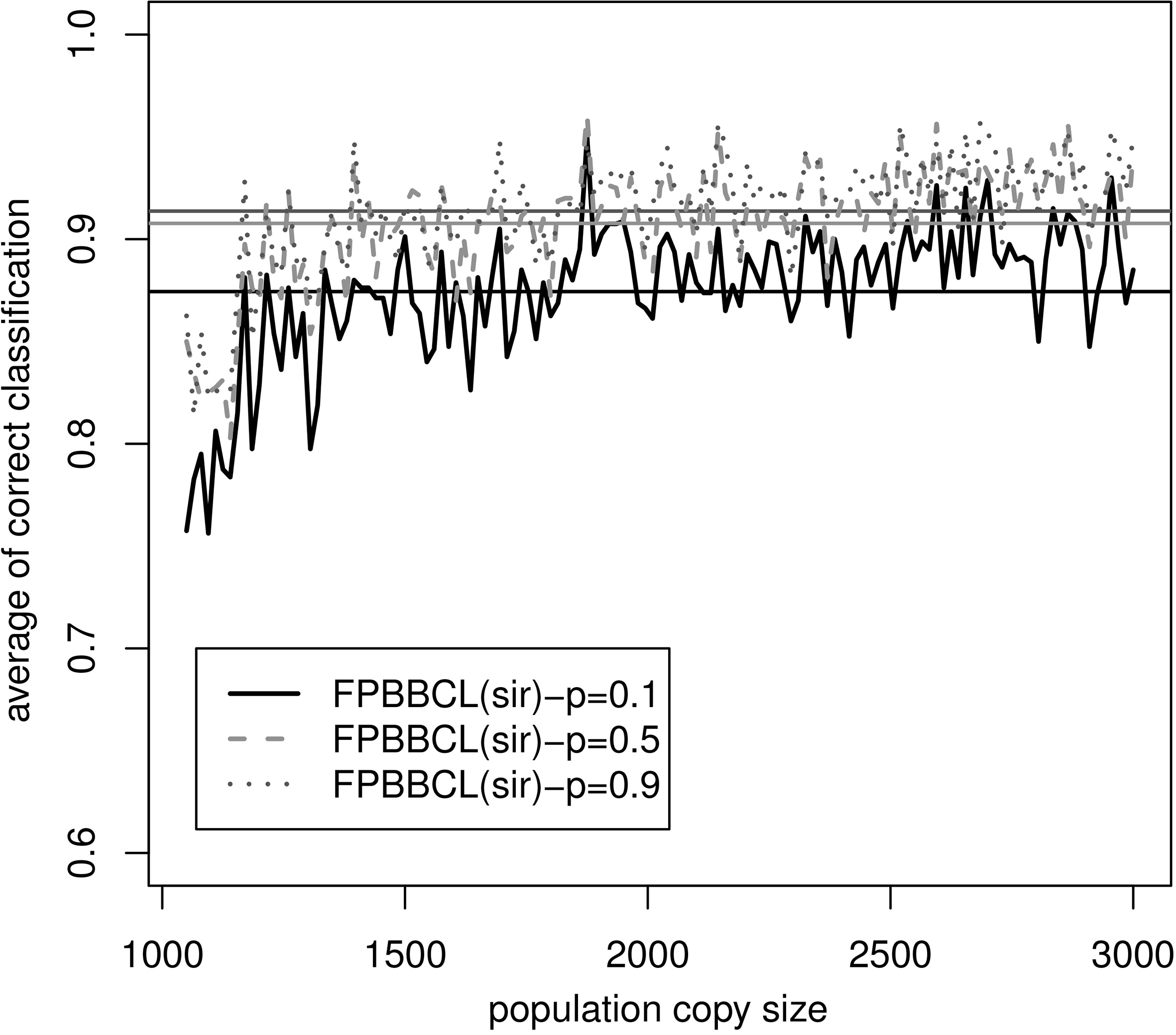$n=$ 50 and $\rho=$ 0.1, 0.5 and 0.9. We choose the first $n$ that has the maximum average of correct classification for each simulation case.

The averages of prediction accuracy of simulated data for the different training sample sizes, different correlations and methods are represented in Table 1. It is generally observed that when the correlation between predictors is low and sample size is small, FPBBLC(sir) has better performance compared to other classifiers. When correlation between covariates increases the average of accuracy improves. For example, when $\rho=$ 0.1 and $n=$ 20, the average of accuracy of FPBBLC(sir) for the test data, is about 83.9% that increases to 92.3% for $\rho=$ 0.9. Because, with respect to the simulation model Eq. (5), as correlation increases the correlation between response variable and linear combination of covarites increase, too.

In general, increasing the sample size $n$ improves the prediction performances of all methods, for instance, when train sample size is 20 and $\rho=$ 0.1, the average of accuracy of the classification rate for FPBBLC(sir) is about 83.9% and increases to 86.5% for the train sample size of 50 with the same correlation. It is notable for FPBBLC(sir) when sample size increases and goes to the Polya sample size, the difference between this method and other classifiers becomes the difference between a traditional logistic classifier and other methods. In addition, $l$ , i.e., the number of Polya sampling iterations can be any integer number between 20 to 40 and results do not significantly differences from this choice. Our experimental observations show that $l=$ 30 cause optimal result.

6.2 Wisconsin prognostic breast cancer data

In this subsection, we compare FPBBLC in three cases to classify the Wisconsin Diagnostic Breast Cancer (WDBC) data set taken from the UCI repository. This data set consists of 569 instances with 30 predictors and diagnosis as a response variable at two levels: malignant and benign. As we emphasized before, SIR needs linearity condition among covariates, thus a Box-Cox Transformation (BCT) is used to fulfill this condition. Therefore, we use BCT on WDBC data and compare our algorithm in two cases with and without dimensionality reduction and in dimensionality reduction with or without BCT. We use suffix BC with FPBBLC(sir) for showing usage of BCT in our algorithm and compare performance of the proposed method with those of some other popular classifiers. Since in WDBC data set, the sample size is equal or bigger than covarites number, we can compare different classifiers with the traditional logistic classifier, which is shown with LR.

Table 2
Comparing FPBBLC(sir) with different classifiers based on the average percent of prediction accuracy for samples obtained from (WDBC) data set at 1000 runs. The best values are bolded

	Training sample size
Method	$n=$ 30	$n=$ 90	$n=$ 180	$n=$ 360
LR	59.9	88.5	91.8	93.9
FPBBLC(sir)	93.0	95.5	96.6	96.8
FPBBLC(sir)-BC	93.2	95.7	96.7	96.7
FPBBLC	89.1	92.1	93.1	94.3
LASSO	91.4	95.1	96.2	96.7
Ridge	82.2	95.0	96.3	96.7
EN	92.0	95.3	96.6	97.3
NB	92.5	93.2	93.6	93.6
KNN ( $k=3$ )	89.2	91.6	92.3	92.5
KNN ( $k=5$ )	89.0	91.4	92.6	92.8

We randomly split WDBC data into two parts train and test data and select four random samples with 30, 90, 180 and 360 instances as training data and reminded data in each case as a test data. We repeat this sampling 1000 times and for every sample, we compare all classifiers and calculate the average of classification accuracy as evaluation criteria. In this case the population copy size is 569, and we iterate each copy 30 times, i.e., $l=$ 30 and results are provided in Table 2.

As we can see in Table 2, both of FPBBLC methods with SIR have better results than FPBBLC without dimensionality reduction because in our algorithm, we use the estimated parameters and estimated base of the CS to predict the class of new data. When the training sample size is small, using BCT causes little improvement in accuracy average. This trend reverses when the training sample size increases. Similar to simulation study, when the training sample size is small, FPBBLC methods based on SIR have a better performance than other classifiers. For example, when the training sample size is 30, the percent of the accuracy average of FPBBLC(sir) is 93%, which is the highest percentage of accuracy in this case excluding FPBBLC(sir)-BC. But, as the training sample size increases, the precision of other classifiers increases more such that EN has the highest accuracy present when the sample size is 360.

In each sample size, LR has the worst performance because the correlation between covariates of WDBC is high and collinearity is possible. Furthermore, when $n=$ 30 and is equal to covariates number, the estimation of parameters is not so precise. This is another advantage of the proposed method rather than traditional logistic classifier.

7. Applications to microarray gene expression data

Here, we compare our proposed methods with other classifiers on three famous gene expression datasets: Colon, Leukemia and Prostate. The Colon data set [1] contains 2000 genes and 62 samples, and tissue type is response variable, which consists of 22 normal tissues and 40 cancer tissues. Leukemia microarray data set [18] includes 7,129 genes and 72 sicks that categorized 47 patients with Acute Lymphoblastic Leukemia (ALL) and 25 patients with Acute Myeloid Leukemia (AML). Liang et al. [25] based on the protocol defined by Dudoit et al. [13] and after doing the filtering, standardizing and using a logarithmic transformation, provided data set comprising 3,571 genes that we used this data for our evaluations. Furthermore, the original prostate data set contains 12,600 genes for 102 tissues, i.e., 50 normal tissues and 52 prostate tumor tissues. Our experiment is based on optimized prostate data [38] that contains 6033 genes and 102 samples.

To evaluate performance of the proposed algorithm, we randomly split datasets into two parts, approximately, 70% for training and 30% for testing. Each procedure is repeated 100 times and the averaged accuracy of prediction, sensitivity, specificity and Standard Deviation (SD) of each index, are reported in Tables 3 to 5. Similar to Liang et al. [25], we select the train/test sample size of Leukemia, Prostate and Colon data 50/22, 71/31 and 42/20 respectively.

Table 3
Percent of accuracy (SD in parentheses) of classification algorithms for Colon gene expression datasets

Algorithm	Predictive accuracy	Sensitivity	Specificity
FPBBLC(sir)	81.1 (0.07)	87.1 (0.11)	70.1 (0.06)
FPBBLC(sir)-BC	81.5 (0.05)	83.5 (0.08)	80.1 (0.10)
LASSO	78.7 (0.08)	90.7 (0.11)	59.6 (0.25)
Ridge	79.5 (0.08)	88.2 (0.09)	65.3 (0.21)
EN	80.1 (0.08)	89.6 (0.05)	66.3 (0.26)
NB	61.0 (0.12)	78.0 (0.13)	45.9 (0.15)
KNN ( $K=$ 3)	80.3 (0.08)	80.6 (0.12)	81.9 (0.14)
KNN ( $K=$ 5)	79.3 (0.09)	77.8 (0.12)	86.5 (0.12)

Table 4

Percent of accuracy (SD in parentheses) of classification algorithms for Leukemia gene expression datasets

Algorithm	Predictive accuracy	Sensitivity	Specificity
FPBBLC(sir)	96.4 (0.04)	93.3 (0.07)	98.3 (0.03)
FPBBLC(sir)-BC	95.2 (0.05)	92.5 (0.10)	96.9 (0.04)
LASSO	92.3 (0.06)	82.8 (0.16)	98.2 (0.03)
Ridge	96.3 (0.03)	91.2 (0.10)	98.3 (0.03)
EN	95.1 (0.05)	88.9 (0.13)	99.2 (0.01)
NB	94.6 (0.04)	91.7 (0.12)	97.3 (0.05)
KNN ( $K=$ 3)	96.3 (0.05)	92.1 (0.10)	98.7 (0.03)
KNN ( $K=$ 5)	94.0 (0.02)	96.4 (0.07)	92.9 (0.03)

Table 5

Percent of accuracy (SD in parentheses) of classification algorithms for Prostate gene expression datasets

Algorithm	Predictive accuracy	Sensitivity	Specificity
FPBBLC(sir)	91.0 (0.05)	93.8 (0.04)	88.5 (0.07)
FPBBLC(sir)-BC	88.7 (0.05)	89.6 (0.08)	87.5 (0.08)
LASSO	89.7 (0.09)	92.2 (0.11)	87.7 (0.13)
Ridge	89.0 (0.04)	92.6 (0.04)	86.5 (0.06)
EN	92.9 (0.04)	95.2 (0.03)	91.4 (0.07)
NB	61.7 (0.10)	63.1 (0.09)	61.1 (0.15)
KNN ( $K=$ 3)	82.0 (0.06)	82.9 (0.08)	81.5 (0.09)
KNN ( $K=$ 5)	84.3 (0.08)	86.0 (0.10)	83.9 (0.12)

As shown in Table 3, for Colon data set, FPBBLC(sir) and FPBBLC(sir)-BC give the average predictive accuracy 81.1% and 81.5%, respectively. Comparing these values with the values of the other classifiers shows that these methods, especially FPBBLC(sir)-BC, are suitable for classification of Colon data set rather than other classifiers. Considering the sensitivity and specificity indices confirms this again. Furthermore, the low amount of SD shows that the suggested method is robust too. Note that since the response variable has two levels, we have one base for each data set, at the result; our methods only use one variable to getting such accuracy. This means that, after calculating the basis of CS with SIR and training the algorithm, using this algorithm to predict the classes of new data, needs less time than other classifiers. With respect to Table 4, for Leukemia data set FPBBLC(sir) and FPBBLC(sir)-BC give the average predictive accuracy 96.4% and 95.2%, respectively. In this case, FPBBLC(sir) has the maximum of accuracy and sensitivity among all classifiers. Furthermore, considering Table 5, gives the similar results. This means that both FPBBLC(sir) and FPBBLC(sir)-BC methods have the credible performance to HDD classification.

Our results show that the linearity condition imposed with SIR, in general, does not have a significant effect on the accuracy of FPBBLC(sir). That is because as Li [24] states often low projections of HDD have approximately the normal distribution, so the linearity condition is not a restrictive condition for our algorithm. Also, the sensitivity and specificity are extremely balanced in our algorithm in comparison with other algorithms. Furthermore, in all cases, the average accuracy of classifying the training data is almost 1 which is significantly better than those of other classifiers.

8. Conclusions

We introduced a new algorithm for the classification of HDD. Our method is based on utilizing traditional logistic regression classifier on a combination of real data and the mean of different resampling data simulated from FPBB. We generate data until the Polya sample size is greater than the number of covariates. Simulation studies and analysis of real microarray data show that our algorithm is more accurate, particularly when the sample size is too small. The proposed algorithm is simple, does not need variable selection that is computer-intensive for HDD, applicable for extremely correlated data and also unbalanced data. The interpretation of why the combined data improve performance, whereas traditional logistic classifier, is not fairly straightforward. However, in the logistic regression classifier, determining class of new data is based on the positive or negative value of $\beta_{0}+\bm{\beta}_{1}^{T}\bm{x}$ . Therefore, if value of $\beta_{0}+\bm{\beta}_{1}^{T}\bm{x}$ , which is calculated from the combination of the Polya sample and real data, is far from zero, we can have a better estimation of parameters in the model Eq. (5). This approximation is valid because in our algorithm this value is completely far from zero. Also, the $p$ -value of Hoslem test of goodness of fit for logistic regression models [21] is greater than 0.9 in all simulations and real data analyses, so the application of traditional logistic regression on the synthetic data is correct.

Footnotes

Acknowledgments

The authors would like to thank anonymous referees for their helpful comments and for careful reading that greatly improved the article.

References

Alon

Barkai

Notterman

Gish

Ybarra

Mack

and Levine

, Broad patterns of gene expression revealed by clustering analysis of tumor and normal colon tissues probed by oligonucleotide arrays, Proc Nat Acad Sci USA 96(12) (1999), 6745–6750.

Bal

Agam

Frieder

and Frieder

, Interactive degraded document enhancement and ground truth generation, in: Document Recognition and Retrieval XV Yanikoglu

B.A.

and Berkner

, eds, Proc. SPIE 6815 (2008).

Bellman

, Dynamic Programming, Princeton University Press, 1957.

Bickel

P.J.

and Freedman

D.A.

, Asymptotic normality and the bootstrap in stratified sampling, Annals of Statistics 12 (1984), 470–482.

Chang

W.C.

, On using principal component before separating a mixture of two multivariate normal distributions, Applied Statistics 32(3) (1983), 267–275.

Chao

M.T.

and Lo

S.H.

, A bootstrap method for finite population, Sankhya Ser. A 47 (1985), 399–405.

Chawla

N.V.

Bowyer

K.W.

Hall

L.O.

and Kegelmeyer

W.P.

, Smote: Synthetic minority over-sampling technique, Journal of Artificial Intelligence Research 16 (2002), 321–357.

Christobel

and Sivaprakasam

, An empirical comparison of data mining classification methods, International Journal of Computer Information Systems 3(2) (2011), 24–28.

Cook

R.D.

, Graphics for regression with a binary response, Journal of the American Statistical Association 91(435) (1996), 983–992.

10.

Cook

R.D.

and Lee

, Dimension reduction in binary response regression, Journal of the American Statistical Association 94(448) (1999), 1187–1200.

11.

Cook

R.D.

and Ni

, Sufficient dimension reduction via inverse regression: a minimum discrepancy approach, Journal of the American Statistical Association 100(470) (2005), 410–428.

12.

Czepiel

S.A.

, Maximum likelihood estimation of logistic regression models: theory and implementation, Available at czep.net/stat/mlelr.pdf, (2002).

13.

Dudoit

Fridlyand

and Speed

T.P.

, Comparison of discrimination methods for the classification of tumors using gene expression data, Journal of the American Statistical Association 97(457) (2002), 77–87.

14.

Efron

, Bootstrap methods: another look at the Jackknife, Annals of Statistics 7(1) (1979), 1-26.

15.

Fienberg

S.E.

, A radical proposal for the provision of micro-data samples and the presentations of confidentiality, Carnegie Mellon University Department of Statistics, Technical Report 611, 1994.

16.

Friedman

Hastie

Hofling

and Tibshirani

, Pathwise coordinate optimization, Annals of Applied Statistics 1(2), (2007), 302–332.

17.

Friedman

Hastie

Hofling

and Tibshirani

, Regularization paths for generalized linear models via coordinate descent, Journal of Statistical Software 33(1) (2010).

18.

Golub

Slonim

Tamayo

Huard

Gaasenbeek

Mesirov

Coller

Loh

Downing

Caligiuri

Bloomfield

and Lander

, Molecular classification of cancer: class discovery and class prediction by gene expression monitoring, Science 286(5439) (1999), 531–537.

19.

Gross

T.S.

, Median estimation in sample surveys, Proceedings of the Survey Research Methods Section (American Statistical Association) (1980), 181–184.

20.

Hoerl

A.E.

and Kennard

R.W.

, Ridge regression: Biased estimation for nonorthogonal problems, Technometrics 12(1) (1970), 55–67.

21.

Hosmer

D.W.

and Lemeshow

, Applied Logistic Regression, Wiley, New York, 2013.

22.

Ichim

, Quantile-based bootstrap method to generate continuous synthetic data, In Proceedings of the 2010 EDBT/ICDT Workshops ACM, 2010.

23.

Lee

Ahn

Moon

Kodell

R.L.

and Chen

J.J.

, Multinomial logistic regression ensembles, Journal of Biopharmaceutical Statistics 23(3) (2013), 681–694.

24.

K.C.

, Sliced inverse regression for dimension reduction, Journal of the American Statistical Association 86(414) (1991), 316–327.

25.

Liang

Liu

Luan

X.Z.

Leung

K.S.

Chan

T.M.

Z.B.

and Zhang

, Sparse logistic regression with a L1/2 penalty for gene selection in cancer classification, BMC Bioinformatics 14(1) (2013), 198 (1–12).

26.

Lim

Ahn

Moon

and Chen

J.J.

, Classification of high-dimensional data with ensemble of logistic regression models, Journal of Biopharmaceutical Statistics 20(1) (2010), 160–171.

27.

A.Y.

, Bayesian statistical inference for sampling a finite population, Annals of Statistics 14 (1986), 1226–1233.

28.

A.Y.

, A Bayesian bootstrap for finite population, Annals of Statistics 16 (1988), 1684–1695.

29.

Meeden

, A noninformative Bayesian approach to small area estimation, Survey Methodology 29(1) (2003), 19–24.

30.

Meeden

Radu

and Charles

J.G.

, polyapost: Simulating from the Polya posterior, R package version 1.5. https://CRAN.R-project.org/package=polyapost, (2017).

31.

Meyer

Dimitriadou

Hornik

Weingessel

and Leisch

, e1071: Misc Functions of the Department of Statistics, Probability Theory Group (Formerly: E1071), TU Wien, R package version 1.6-8. https://CRAN.R-project.org/package=e1071, 2017.

32.

Nonnemaker

and Baird

H.S.

, Using synthetic data safely in classification, in: Proc. SPIE 7247, Document Recognition and Retrieval XVI, 72470G, 2009.

33.

Sanford

, Dimension reduction regression in R, Journal of Statistical Software 7 (2002), 1–22.

34.

Tibshirani

, Regression shrinkage and selection via the lasso, Journal of the Royal Statistical Society: Series B (Methodological) 58(1) (1996), 267–288.

35.

Varga

and Bunke

, Effects of training set expansion in handwriting recognition using synthetic data, in: In 11th Conf. of the International Graphonomics Society, Citeseer, (2003), 200–203.

36.

Varga

and Bunke

, Comparing natural and synthetic training data for off-line cursive handwriting recognition, in: Frontiers in Handwriting Recognition (2004), 221–225.

37.

Wang

Chen

, Huang

and Feng

, Scalable subspace logistic regression models for high-dimensional data, APWeb 2012, LNCS 7235 (2012), 685–694.

38.

Yang

Cai

Z.P.

J.Z.

and Lin

G.H.

, A stable gene selection in microarray data analysis, BMC Bioinformatics 7(1) (2006) 228 (1–16).

39.

Zhang

Zang

Sigal

and Agam

, Learning classifiers from synthetic data using a multichannel autoencoder, arXiv:1503.03163, 2015.

40.

Zou

and Hastie

, Regularization and variable selection via the elastic net, Journal of the Royal Statistical Society: Series B (Statistical Methodology) 67(2) (2005), 301–320.

Finite population Bayesian bootstrapping in high-dimensional classification via logistic regression

Abstract

Keywords

1. Introduction

2. Related work

3. Bayesian bootstrapping in a finite population

4. Sliced inverse regression

6.1 Simulation analysis

Table 2 Comparing FPBBLC(sir) with different classifiers based on the average percent of prediction accuracy for samples obtained from (WDBC) data set at 1000 runs. The best values are bolded

Table 3 Percent of accuracy (SD in parentheses) of classification algorithms for Colon gene expression datasets

Footnotes

Acknowledgments

References

Table 2
Comparing FPBBLC(sir) with different classifiers based on the average percent of prediction accuracy for samples obtained from (WDBC) data set at 1000 runs. The best values are bolded

Table 3
Percent of accuracy (SD in parentheses) of classification algorithms for Colon gene expression datasets