The search of conditional outliers

Abstract

There is no standard definition of outliers, but most authors agree that outliers are points far from other data points. Several outlier detection techniques have been developed mainly for two different purposes. On one hand, outliers are considered error measurement observations that should be removed from the analysis, e.g. robust statistics. On the other hand, outliers are the interesting observations, like in fraud detection, and should be modelled by some learning method. In this work, we start from the observation that outliers are affected by the so-called simpson paradox: a trend that appears in different groups of data but disappears or reverses when these groups are combined. Given a data set, we learn a regression tree. The tree grows by partitioning the data into groups more and more homogeneous of the target variable. At each partition defined by the tree, we apply a box plot on the target variable to detect outliers. We would expect that the deeper nodes of the tree would contain less and less outliers. We observe that some points previously signalled as outliers are no more signalled as such, but new outliers appear.

Keywords

Outliers conditional outliers boxplot analysis regression tree simpson’s paradox

1. Introduction

Data science is a field in constant and rapid evolution. More than ever before we are aware that, acquired knowledge from any data set allow us, not only to understand, but also to predict observations behavior. Normally we aim to identify relevant patterns among populations, but sometimes the most valuable information is not in the general pattern but in the deviant behaviors. Such uncommon observations, denominated as outliers, may be mere errors in measurement or may represent very important observations with very particular features of interest. Sometimes this kind of observations may not be so obvious as they are being intentionally disguised, for example, when trying to cover fraud. Geology studies or public health services are other fields which make the study of methods for outlier detection a matter of interest. There are different kinds of outliers and the technique we choose to use will depend on it. In this paper we propose a method to search for different contexts, in which we can uncover extreme outliers, regarding one specific variable of interest – target variable. Each scenario is chosen based on the other known variables that are used to divide the data in groups as homogeneous as possible. We also propose a score measure to assign to each observation. Using these results, we will point out that outlier detection may be an example of simpsons paradox [1]: a trend that appears in divided sets of data and reverses or disappears when combining them.

The paper is organized as follows: Section 2 introduces important definitions and related work regarding outlier detection; Section 3 presents the problem formulation; Section 4 shows our approach to to the problem; Section 5 presents the experimental results showing an illustrative example to explain the workflow of our method and a comparison of the results of our method and two baselines using a real life data set of a retail company [2], and in two known data sets; finally, in Section 6 we present the conclusions of this work.

2. Related work

2.1 Outlier definition

Outliers are observations that are considered abnormal. Hawkins [4] formally defined: “An outlier is an observation which deviates so much from the other observations as to arouse suspicions that it was generated by a different mechanism”.

Depending on the nature of the outlier, Singh and Upadhyaya [5] classified them as:

•
Point outliers. The simplest type of outliers, a mere observation that falls away from the other observations. It may be a measurement error or an abnormal behavior/feature of the individual. For instance, a high quantity of water consumed in a month in a house may suggest a broken pipe or other problem in the infrastructure.
•
Contextual outliers. Also known as conditional outliers, this term refers to observations that are only detected as outliers in a certain context. For instance, let us take the usage of electricity of individuals in a town. If a house presents abnormally high consumption, it may go unnoticed among the entire population because the normal consumption in the industries is probably higher anyway. But, if we focus on domestic context we can easily detect it.
•
Collective outliers. Outliers may not be an individual record but a collection of values in a certain order. For example, let’s consider a person’s daily travel distance and assume this individual travels a longer path on working days than in the weekends. If for seven consecutive days this person shows a shorter travel distance and after that returns to the usual distance, we may assume that, for some reason, this person did not go to work that week. So, the distance values were not considered outliers as they were normal for the weekends. It is the fact that they appear for 7 consecutive observations that is considered abnormal.

When looking for outliers, we must be aware of two possible situations: masking and swamping effect. These situations may disguise some outliers [6]. Both occur when deviant observations skew the mean and the covariance estimated towards it.

Masking effect occurs when a deviant observation $a$ is not considered as outlier because other abnormal observation $b$ is influencing the mean and the covariance in the direction of observation $a$ . In other words, if the observation $b$ is removed, observation $a$ will be considered an outlier. In this case, outlier $a$ is masked by outlier $b$ .

Swamping effect occurs when a deviant observation $a$ , is considered an outlier only in the presence of other abnormal observation or observations. The influence of these may skew the mean and covariance towards it and make observation $a$ seem like an outlier when in fact it is not.
2.2 Outlier detection techniques

Different kinds of outliers require different detection methods. We can find in the literature many outlier detection techniques. Hodge and Austin [7] as well as Chandola et al. [8] or Aggarwal [9] summarize the most important of them. From those, we refer the statistic-based, proximity-based and clustering techniques. We also refer to studies conducted to specifically detect contextual outliers.

2.2.1 Statistical-based Techniques

Statistical-based techniques are divided in parametric if it is assumed that the variable follows a known distribution, and non-parametric when there is no assumption to be made as to the distribution of the variable.

Depending on the number of variables one may divide these techniques in univariate (if search is done in only one variable), or multivariate, if we take in consideration two or more variables.

Two simple methods for univariate outlier detection are described next.

•
Boxplot analysis. Point Outliers, as mentioned before, are abnormal observations. In case of numeric variables, these observations have values that are much lower or much higher than most of the others. The most common way to identify them is by Boxplot analysis. We take the interquartile range, ( $\textit{IQR}=Q_{3}-Q_{1}$ ) and consider as outliers the observations that fall farther than $1.5\textit{IQR}$ up the third quartile or down the first quartile. If this distance is $3\textit{IQR}$ , the outliers are considered extreme.
•
Standard deviation analysis. When data are normally distributed presents an empirical behavior where 99.7% of the observations fall within a distance of three standard deviations (3 $\sigma$ ) from the mean ( $\mu$ ), 95% within a distance of 2 $\sigma$ and 68% within a distance of $\sigma$ . When it is possible to assume the data are normally distributed, the standard deviation can be used as an outlier detection measure. Choosing $a$ ( $a\in\Re$ , $a\geqslant$ 1), according to the nature of the data and the goal of the analysis, observations that fall $a\sigma$ away from the mean are considered outliers [10].

2.2.2 Proximity-based techniques

Two of the most known types of outlier detection techniques are distance-based and density-based, which are succinctly described next.

•
Distance-based analysis. General distance-based techniques define outliers according to the distance to the $k$ nearest neighbor. There is no need to have previous knowledge about the data distribution model. These methods assume the $k$ nearest neighbor distance is much larger in outliers than in normal data. The most common used distances are Euclidean or Mahalanobis. These techniques have simple implementations but show an exponential computational growth with the increase of dimension and number of records to compute. Cell-based methods or Index-based methods are examples of Distance-based techniques. Detail of this and other methods are presented in [11].
•
Density-based analysis. Distance-based techniques may be sensitive to data locality. If we divide a data set into clusters, being some of them much sparser then the others, observations may be wrongly considered as outliers or may go unnoticed. If the define distance is too small, many points in the sparser cluster may be considered outliers; if it is too large, an observation that is far away from a denser cluster, comparing to the observations within that cluster, will not be considered abnormal. To overcome this problem, density based algorithms appeared. One example is LOF – Local Outlier Factor, devoloped by Breunig [12], which assigns to each observation a score. This score is the average of the density of the instance and its $k$ neighbors. The density of an instance is calculated dividing $k$ by the volume of the hyper-sphere centered in the instance and with the smallest radius possible to contain the $k$ neighbors.

2.2.3 Clustering techniques

Although the use of clustering algorithms for the detection of outliers being more of a side effect than a goal itself, they may serve this purpose in a satisfactorial way. Assuming that a normal observation is in a cluster, close to the centroid of the cluster, or belongs to a large and dense cluster, we may define as outlier any observation that lies otherwise. A cluster with few observations in it, may be considered a group of outliers. However, it is a hard task to distinguish outliers from noise. Examples of clustering algorithms are K-means, k-medoids or K-NN wich use for instance Euclidean or Mahalanobis distance. Papers [7, 8] summarize the techniques mentioned as well as optimisation specially in what comes to running time and memory issius.

2.2.4 Contextual/conditional outlier detection

There are several outlier detection techniques with the specific goal of finding contextual outliers. We will briefly refer two of those.

Song et al. [13] propose an approach to detect anomalies that starts with the division of the variables of the data set in environmental and indicators attributes. The environmental attributes define different contexts and each observation is evaluated depending on the context. A statistical model is created to represent the data. It consists of a Gaussian Mixture Model to model the set of environmental attributes, an additional set of Gaussians to model the indicator attributes and a probabilistic mapping function between this two sets of Gaussians. The three algorithms presented to learn the model are based on the Expectation Maximization Algorithm for parameters estimation.

Also dividing the variables in contextual and indicative, Liang and Parthasarathy [14] present an approach (ROCOD) that uses weight combination of two measures: Local Expected Behavior and Global Expected Behavior. The first one refers to the average values of behavioral attributes of observations similar to each other in what comes to contextual variables. The second is computed using all the observations, learning regression models that use contextual attributes as input and each of the behavioral attributes. This approach aims to overcome the limitations of applicability presented by other approaches, in what comes to sparsity of the contexts. In both approaches there is the necessity of the user to choose the attributes that define the context.

3. Problem formulation

Let us assume a variable of interest $Y$ whose domain is $\Re$ . Our goal is to analyze this variable regarding its outlier values. For this purpose, several well known techniques are available in the literature. Let us represent the “outlierness” of variable $Y$ as Out(Y). If we want to go deep in the analysis, we might be interested in understanding why a given $y_{i}\in Y$ value is an outlier.

Still, rather than detecting outliers in a set of user pre-defined set of contextual variables, we aim to detect outliers in a target numeric variable using for that purpose other variables as context information to group the individuals of the population.

Thus, we can collect other variables that provide contextual information about the $y_{i}$ . Let us assume we can measure a contextual variable $X_{k}$ by taking values in a discrete or continuous domain $\{x_{k1},x_{k2},\ldots,x_{kn}\}$ . Given the contextual variable $X_{k}$ , we can analyze the distribution of the target variable $Y$ given the values of $X_{k}$ . For example, if $Y$ is Customer Satisfaction and $X_{k}$ represents regions with domain $\{\textit{North},S\textit{outh},\textit{East},\textit{West}\}$ , we can analyze the “outlierness” of Customer Satisfaction per region: Out(Customer Satisfaction $|$ Region) or $\textit{Out}(Y|X_{k})$ , obtaining a finer granularity analysis of the “outlierness” of a given $y_{i}$ value.

Assuming two contextual variables $X_{1}$ , $X_{2}$ with a domain of cardinality $k$ and $j$ respectively, we can analyze $\textit{Out}(Y|X_{1})$ , $\textit{Out}(Y|X_{2})$ or $\textit{Out}(Y|X_{1},X_{2})$ . The number of subsets we obtain is $k$ , $j$ and $k\times j$ , respectively. Given several contextual variables, we can extend our analysis to the subsets of $Y$ given by all possible combinations of the contextual variables. Of course, this is problematic due to the exponential number of possible combinations.

For this specific problem, the data set division must consider all the variables in the data set but there has to be an optimization criteria concerning the target variable while using the other variables to define possible contexts to test the mentioned optimization function.

Methods mentioned in Section 2.2 are designed to detect global outliers that use variables equally or divide the variables in indicators and contextual. The indicator variables do not have an influence on the groups created by contextual variables.

4. Our approach

Our goal is to find outliers regarding one variable when dividing the data set according to the other variables. These subsets should be well defined for results interpretation purpose. Next, we explain how the data partitioning is done. Based on the obtained partitions, we then explain how we assign a “outlierness” score to each observation of the target variable. This work is a large extension of our previous work [3].

4.1 Partition the data into different contexts

As mentioned before, data partition may lead to exponential combinations of subsets. To avoid so, and as we are targeting specifically one variable to detect outliers, we learn a regression tree for this variable using as explanatory variables the contextual ones. A regression tree grows by selecting the explanatory variables that present the higher reduction of the variance in the target variable. This way, we obtain subsets of growing homogeneity in terms of variance of $Y$ .

To learn the regression tree we will use the CART (classification and regression trees) algorithm, Breiman [15], from 1984. The basic idea is, at each node, to choose the best (binary) split based on the decreasing of the variance of the target variable. Depending on the target variable type, categorical or continuous, we have classification trees or regression trees, respectively. The splits are defined by the predictor variables. They also can be categorical or continuous. In the categorical case, the number of possible splits depends on the number of categories, if there are $C$ categories we can define $2^{C-1}-1$ different splits. On the continuous case, as well as the ordinal categorical, the different values are sorted by ascending order and a partition can be made between any two different values.

The tree growth consists in the recursive partitioning of the tree from the root until a stopping criterion is reached. This happens repeating the following steps:

1.
at each node compute the possible splits and choose the better one for each predictor variable;
2.
from the results of 1) choose the better split for the node;
3.
if a stopping criterion is not satisfied, divide the node using the result in 2).

The best split is the one that maximizes the splitting criterion. In the case that the target variable is continuous the goal is to decrease the variance of the target variable. It starts by computing the sum of squares for each node $t$ , starting in the root, $\textit{SS}_{t}=\sum{(y_{i}-\overline{y}_{t})^{2}}$ being $y_{i}$ the value that the target variable takes for observation $i$ and $\overline{y}_{t}$ the mean value in that node. This value is then compared to the sum of squares of the two child nodes, left (tL) and right (tR), $\textit{SS}_{\textit{tL}}+\textit{SS}_{\textit{tR}}$ . The partition that minimizes this sum, maximizes the difference $\textit{SS}_{t}-(\textit{SS}_{\textit{tL}}+\textit{SS}_{\textit{tR}})$ and, therefore is chosen.

There are different stopping criteria that may or may not be user defined. If the observations in a node present identical values for the target variable (pure node) or for the predictor variables the node will not be split. As for user defined parameters we have the depth of the tree, the minimum node size for a splitting takes place, a minimum size for each child node and a minimum to the improvement of the best split. The use of the regression tree provides automatically different scenarios that change as the tree grows. This way we will know which observations are abnormal at each context.
4.2 Detecting and scoring outliers

In this paper, we propose a method to detect outliers and assign score values to them. The goal is to measure the “outlierness” of an observation $i$ in the target variable $Y$ considering the contextual variables $X_{1},\ldots,X_{k}$ used in the regression tree learned. We propose BoxplotTree (cf. Algorithm 1), a contextual outlier detection method where every variable is assumed to be contextual with the exception of the target variable.

[h] Input:

Output:

Initialize:

$T\leftarrow\textit{CART(D)}$

node $t$ in $T$ $D_{t}\leftarrow$ partition of $D$ defined by node $t$

$n_{t}\leftarrow$ nr. observations of $D_{t}$

$Out_{t}\leftarrow\{i\ |\ y_{i}\ \text{is boxplot extreme outlier of }Y\text{ % in }D_{t}\}$

$\tilde{y}_{t}\leftarrow$ median value of target variable $Y$ in $D_{t}$

$sd_{t}\leftarrow$ standard deviation of target variable $Y$ in $D_{t}$

$L_{t}\leftarrow$ level of node $t$

$\langle\mathbf{x}_{i},y_{i}\rangle\in D_{t}$ $\displaystyle\textit{Dist}(y_{i},t)=\frac{|y_{i}-\tilde{y}_{t}|}{sd_{t}}$

$\displaystyle\textit{wDist}(y_{i},t)=\frac{n_{t}}{N}\times Dist(y_{i},t)\times K% ^{L_{t}}$ , where $K\in]0,1[$

$i\notin Out_{t}$ $\textit{wDist}(y_{i},t)=-\textit{wDist}(y_{i},t)$

$OutScore(i)=\textit{OutScore(i)}+\textit{wDist}(y_{i},t)$

$\{OutScore(i)\}_{i=1}^{N}$

BoxplotTree Algorithm

Given a regression data set $D=\{\langle\mathbf{x}_{i},y_{i}\rangle\}_{i=1}^{N}$ , we build a CART regression tree. Then, as an observation may be considered an outlier in some nodes of the tree but not in others, we go through every node in the tree to calculate the “outlierness” score of each observation. With data partition $D_{t}$ defined at each node $t$ , we obtain for the target variable $Y$ : the set of observations that, according to the boxplot definition, are regarded as extreme outliers ( $\textit{Out}_{t}$ ), the median value ( $\tilde{y}_{t}$ ) and the standard deviation ( $sd_{t}$ ). Then, for each observation $\langle\mathbf{x}_{i},y_{i}\rangle\in D_{t}$ , we compute $\textit{Dist}(y_{i},t)$ , the distance of the target variable value $y_{i}$ to $\tilde{y}_{t}$ , and normalize it dividing it by $sd_{t}$ . We then calculate the weighted distance $\textit{wDist}(y_{i},t)$ by weighting these distances using the fraction of observations in the node ( $n_{t}/N$ ) and multiplying it by a power of a constant $K\in\ ]0,1[$ . The exponent of $K$ corresponds to the level of the node in the tree ( $L_{t}$ ), so the score value also depends on the depth of the node the observation fell in.

The “outlierness” score assigned to each observation $i$ is the sum of their correspondent weighted distances, across all the nodes in the tree Still, if the observation under analysis is not regarded as an outlier at a specific node $t$ , i.e. $i\notin\textit{Out}_{t}$ , then we consider that this should decrease its “outlierness” factor. Thus, in these cases, its this weighted distance will take a negative sign. At the end, only observations with a positive score will be considered as outliers.

5. Experimental study

In this section, we present the results of the method previously described applied to a data set of a retail company regarding transaction of returned items. We also propose an experimental setup to validate our method and discuss the obtained results.

5.1 An illustrative example – fraud detection

This data set was the case study of [2]. The data refers to a large real-world retail company. The goal is to identify unusual cases that may suggest the occurrence of fraud in the returning of items process. For that purpose, and in order to make the inspection process effective, the identified outliers should be ranked by a score. We believe that this case study is one intuitive example in what comes to understand the importance of the context in an outlier detection problem.

The provided data set contains information on transactions of returned items collected in a three month period in fourteen different stores. At all we have 43206 transactions correspondent to the period from December of 2014 to February of 2015. Notice that in the respective period there are two days (December, 25th and January, 1st) on which the stores were closed to the public.

Table 1 summarizes the available variables for our analysis. To each observation is associated the total number of returned items as well as its average value when they happen in the exact same conditions. Meaning that each line represents a unique combination of Supervisor, Store, Region, Weekday, Period and Product Type. To each one of the combinations are associated the values of the target variables.

Table 1
Fraud detection data set variables description

Variable	Description
Supervisor	Code of the supervisor from the total of 887 supervisors.
Store	Code of the store from the total of 40 stores.
Region	Region of the store North, Center, South.
WeekDay	Type of day: Business days, Weekend or Holidays.
Period	Period of day : Morning, Afternoon, Night
ProdType	Product type: there are 18 different product types, such as
	Bakery, Fruits and Vegetables, Drink, Entertainment, etc.
TotalNr	Total number of items returned by the supervisor.
AvgVal	Average value of the items returned by the supervisor.

To understand how fraud may occur, we must know how the return items process takes place. Any customer is entitled to return an item if it is not satisfied with it as long as the item is in perfect condition, the establish period of devolution is not over and the proof of purchase is presented. At the store, a supervisor makes the return registration and reimburses the customer. In this process, fraud may occur in two different setups: one happens if the return process is fictitious, meaning there is no customer returning anything and the supervisor makes a refund to his advantage; another one is when the process occurs normally, the customer is reimbursed but the supervisor illicitly keeps the returned item for himself. In both cases there is no physical return of the item to the store although it will be an input to the theoretical stock.

5.1.1 Fraud detection – univariate analysis

Let us start with the univariate analysis of the variables TotalNr and AvgVal which correspond to the total number of returned items and their respective average value. We compute the basic statistics in order to know a little bit more about the target variables mentioned (see Table 2). In both cases the mean value is higher than the median value which suggests a right skewed distribution. Also, in both cases, the IQR is only a small fraction of the Range. At least 50% of the values vary in a very small interval. The outliers represent between 3% and 4% of the total number of observations. Figure 1 shows the boxplot of the variables. We can see that both variables have a high dispersion of values. Both also present a tremendous amount of extreme outliers. But may this outliers be reliable in what comes to suspicion of fraud? It is natural to think that with the discrepancy of prices between product types, the most expensive ones as well as the cheaper ones will be detected as extreme outliers. In the other hand, it is intuitive to expect that the number of returned items will be higher in a period of high affluence to the store. These are only two possible contextualization combinations.

Table 2
Basic statistics measures of TotalNr and AvgVal

Variable	Min	1 ${}^{\text{st}}$ Qu	Median	Mean	3 ${}^{\text{rd}}$ Qu	Max	SD	Range	IQR	Outlier count
TotalNr	1	2	4	9.34	11	725	14.59	724	9	1695
AvgVal	0.02	2.48	4.64	8.26	9.47	1167	14.07	1167.1	6.99	1480

Figure 1.

Boxplot analysis for the univariate detection of outliers in the target variables.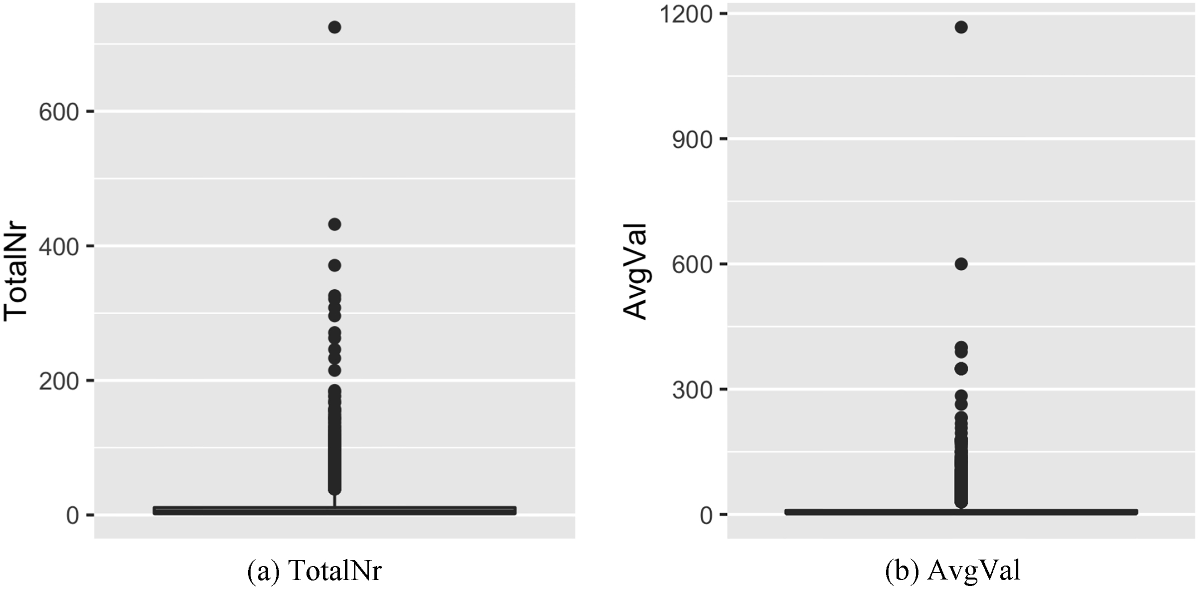

5.1.2 Fraud detection – boxplottree analysis

As mentioned before, the possible number of combinations when using the contextual variables to divide the data set and provide different contexts to each subset of variables may be exponential. To overcome this, as described in the previous section, we learned a regression tree for each one of the target variables using the categorical variables. We choose the CART algorithm [15], which is one of the best known algorithms and it is implemented on rpart package [16] using R language [17]. To illustrate the result, Fig. 2 shows the learned tree until depth four of the target variable TotalNr. At each node we can see information about the number of observations, the number of extreme outliers, and, how many of them were considered as such at the father node. As the tree grows, outliers “appear” and “disappear”. Each node represents a different context so the same observation may be considered as an extreme outlier in one node but not in the others. This figure exemplifies how easy it is to the final user the interpretation of the contexts generated by the regression tree.

To better illustrate the example, Table 3 presents information for five different observations about $\textit{Dist}(y_{i},t)$ , i.e. the distance to the median normalized by the standard deviation of a node $t$ , considering all nodes until the fourth level of the tree.

Table 3
$\textit{Dist}(y_{i},t)$ for target variable TotalNr and considering a tree depth of 4

Obs ID	Root	1	2	3	4
220	2.40	3.20	$-$ 1.96	$-$ 1.57	$-$ 1.21
252	2.47	$-$ 1.67	$-$ 1.10	$-$ 0.80	$-$ 0.90
269	9.05	6.54	4.69	$-$ 3.77	3.87
1022	3.56	2.48	2.99	$-$ 2.42	$-$ 2.03
1460	$-$ 1.85	2.47	3.55	3.03	$-$ 2.53

Figure 2.

BoxplotTree analysis on TotalNr.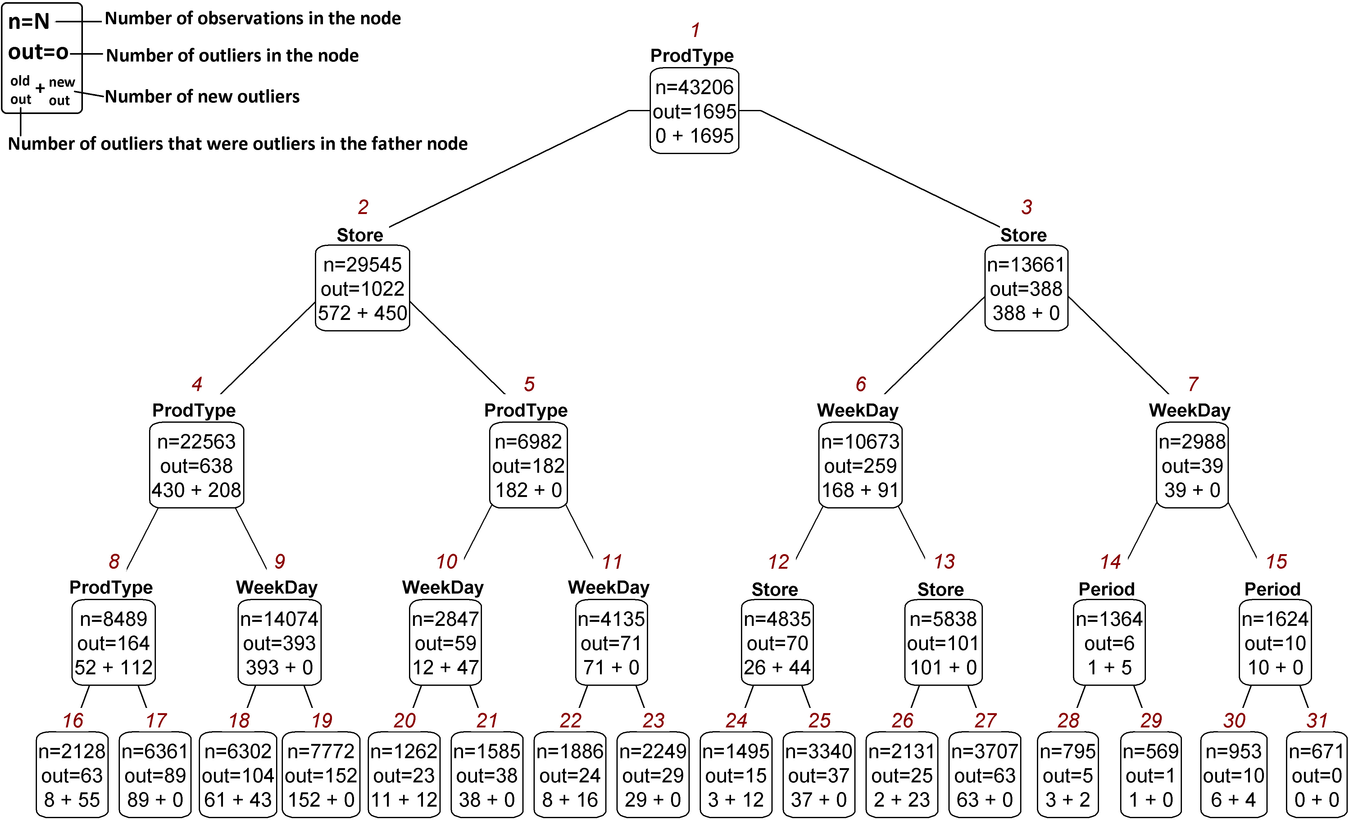

A negative value means that the observation was not considered extreme outlier at the level correspondent to the column. Observations 220 and 252 stopped being considered as extreme outliers after levels two and one respectively. Observations 269, 1022 and 1460 “appear” and “disappear” as outliers along the tree. Notice that observation 1460 was detected as extreme outlier for the first time at level one.

In what comes to assign a score value, we follow the BoxplotTree method described in Algorithm 1. For the regression tree we set cp $=$ 0 and maxdepth $=$ 5. This way, any split of the tree will take place even for very low improvements with respect to the total variance. Moreover, considering that $K$ parameter only takes values between 0 and 1, we considered that its powers may be disregarded from level five forward as they get very low. All the other rpart [16] parameters were left by default.

In order to have a comparison baseline, we compute the difference to the median normalized by the standard deviation of the extreme outliers detected with a simple Boxplot analysis.

Let us illustrate the process of wDist score calculation using the example of transaction 22152 that presents a TotalNr of 725. Table 4 shows the values we use for this purpose. This observation was considered as an extreme outlier at all the nodes. Each column refers to one level of the tree. The second line shows the node $t$ at which the observation fell at each level. To calculate the score at each level, we subtract the median value of each node $\tilde{y}_{t}$ from the target value of the observation $y_{i}$ and divide the result by the standard deviation of the node $sd_{t}$ . The obtained value is now multiplied by the fraction of observations of the correspondent node ( $n_{t}/N$ ). This way, more importance is given to the nodes with higher quantity of observations. After this process, we set $K=$ 0.5 and multiply the previous result by the correspondent K power ( $K^{L_{t}}$ ) so that at each level the score is reduced. The last line, shows the wDist score at the correspondent level. Finally, we sum all the values in the last line to assign the outlierness score for observation 22152, and obtain $\textit{OutScore}(22152)\approx$ 58.63. This transaction is considered as an extreme outlier since presents a positive score.

Table 4

wDist calculation for transaction $i=$ 22152 with a TotalNr target value $y_{i}$ of 725 returned items

Level $L_{t}$	0 (Root)	1	2	3	4	5
Node $t$	1	3	6	13	27	54
$\tilde{y}_{t}$	4	7	6	7	8	7
$sd_{t}$	14.590	19.720	16.700	20.230	23.620	23.080
$n_{t}/N$	1.00	0.316	0.247	0.135	0.086	0.050
$K^{L_{t}}$	1	0.500	0.250	0.125	0.062	0.031
$\textit{wDist}(y_{i}.t)$	49.407	5.755	2.658	0.599	0.163	0.049

Table 5 shows the first twenty observations ranked by BoxplotTree as well as the variable value and the score value assigned to the the observations using the same method but considering only extreme outliers detected by a simple Boxplot. The rank is presented between parenthesis.

We can observe that the observations are ranked differently by the two methods. BoxplotTree increases the importance of the observations that were considered extreme outliers in other tree levels besides the root. Notice observation 28442 who occupied the 3 ${}^{\rm rd}$ position with Boxplot dropped to 7 ${}^{\rm th}$ with BoxplotTree. Other observations became more suspicious than this one. Observations 23775 and 37181 were ranked lower than 20 ${}^{\rm th}$ by Boxplot but not by the BoxplotTree.

Table 5

Scores and rank values by Boxplot and BoxplotTree for the target variable TotalNr

Obs ID	TotalNr	Boxplot	BoxplotTree	Obs ID	TotalNr	Boxplot	BoxplotTree
22152	725	49.41 (1)	58.63 (1)	12545	215	14.46 (12)	21.79 (11)
15208	326	22.07 (4)	33.16 (2)	8654	271	18.30 (8)	21.68 (12)
14673	432	29.33 (2)	33.09 (3)	33984	263	17.75 (9)	20.01 (13)
39896	321	21.72 (5)	32.64 (4)	37956	185	12.40 (13)	18.63 (14)
19032	308	20.83 (6)	31.31 (5)	21034	184	12.33 (14)	18.53 (15)
39635	296	20.01 (7)	30.07 (6)	23775	154	10.28 (26)	18.37 (16)
28442	371	25.15 (3)	28.37 (7)	3265	177	11.85 (16)	17.81 (17)
24934	246	16.58 (10)	24.99 (8)	17041	170	11.38 (18)	17.09 (18)
35056	233	15.69 (11)	23.58 (9)	37181	144	9.59 (32)	14.41 (19)
25703	182	12.2 (15)	21.92 (10)	12218	176	11.79 (17)	13.28 (20)

In order to get a real conclusion as if fraud is occurring or not, a deeper inspection is needed. The presented method is only a tool that suggests suspicious observations not only by the abnormal value they may present but also by their capacity to integrate a group with similar characteristics and not be considered as an extreme outlier.

Due to the sensitive of the matter, the access to the ground truth of the fraudulent transactions in this real life case was denied to authors of this paper. However, the fact that instances that were detected as extreme outliers in higher levels of the tree were observations of interest was confirmed.

5.2 Results validation

As it is very difficult to obtain data sets with ground truth results regarding outlier detection, we propose the following experimental setup to validate the effectiveness of our method. We use a 10-fold cross validation method to compare the mean absolute error of predictions made by rpart [16] when no observation is removed from the training set and when outliers detected by some baseline methods and by BoxplotTree are withdrawn from the training set. Our assumption is that removing outliers from a training set should, in principle, improve the predictions and thus reduce the error of the model.

As baseline methods, we use the Boxplot analysis and LOF. At each iteration, we compare the Mean Absolute Error (MAE) of the predictions obtained when using as training set:

•
all observations;
•
all observations except the ones considered severe outliers by the Boxplot;
•
all observations except the outliers detected by BoxplotTree;
•
all observations except the outliers detected by LOF.

Table 6
Number of outliers in common detected by Boxplot (BP), BoxplotTree (BPTree) and LOF

BP % BPTree % LOF % BP and BPTree BP and LOF BPTree and LOF

1 1532 3.94 1624 4.18 843 2.17 1532 38 39

2 1524 3.92 1616 4.16 857 2.20 1524 36 36

3 1520 3.91 1613 4.15 833 2.14 1520 35 35

4 1531 3.94 1613 4.15 827 2.13 1531 35 35

5 1507 3.88 1590 4.09 856 2.20 1507 35 35

6 1515 3.90 1592 4.09 864 2.22 1515 31 31

7 1520 3.91 1565 4.02 846 2.18 1520 36 36

8 1531 3.94 1620 4.17 842 2.17 1531 34 34

9 1546 3.98 1618 4.16 841 2.16 1546 33 33

10 1529 3.93 1603 4.12 774 1.99 1529 32 32

Besides the Fraud data set described in Section 5.1, we also performed experiments on UCI data sets Housing and Energy Efficiency described below.

•
Housing data set: data set used in the CART book [15]. The regression problem consists of predicting the house value in the suburbs of Boston. We use the version of the data set available at the UCI repository [18]. It consists of 506 instances evaluated in 14 variables, 12 of them continuous, 1 binary and the target variable, “MEDV” which is the house value.
•
Energy efficiency: data set created by Angeliki Xifara and processed at University of Oxford, UK [19]. It consists of 768 instances (buildings) characterized by eight real and integer variables. There are two target variables – “Heating Load” and “Cooling Load”. Due to redundant results in what comes to outlier detection we chose to show the “Cooling Load” results.

Regarding the outliers detected by the Boxplot Analysis, we consider only the extreme ones as explained in Section 2.2.1. As for LOF, due to the fact that it takes a long time to process the score values with a large number of neighbors, we decide to use only 3 neighbors. For each data set the score value was chosen based on a percentage of outliers of approximately 4% of the data set instances. We chose the MAE to compare the predictions of the four cases mentioned above since it is more robust to the presence of outliers.

Figure 3 shows the distribution of OutScore values assigned by the BoxplotTree at one of the iterations for the four regression problems. The results of the ten iterations were all very similar. As expected, most scores present a negative value, meaning that they were not considered as outliers at any level of the regression tree, or they were considered as outliers in some context but the value was not very significant. The tendency is to a very small quantity of observations present score values above zero. The Energy Efficiency data set does not present any score above zero for any of the ten training sets. So, from this point forward, we are not going to consider this data set for the experiments.

Table 7
P-value for the Wilcoxon Signed Rank Test performed on the results obtained by considering the all the observations (O) and removing the oultliers detected by Boxplot (BP), BoxplotTree (BPTree) or LOF

Fraud Nr Fraud AV Housing

O $>$ BP 0.0029 0.0010 0.6152

O $>$ BPTree 0.0020 0.0010 0.6152

O $>$ LOF 0.2158 0.0186 0.4609

BP $>$ BPTree 0.0322 0.0322 –

LOF $>$ BP 0.0029 0.0010 0.6523

LOF $>$ BPTree 0.0020 0.0010 0.6523

Figure 3.
OutScore distribution regarding the target variable of each data set obtained by BoxplotTree.

Lets start the analysis of the results by comparing the outliers detected by each method. If we observe Table 6, we see that BoxplotTree detects the outliers detected by Boxplot and more. However, LOF detects only 38 and 39 outliers in common with Boxplot and BoxplotTree, respectively.

The results for the same data set but the target variable “AvgVal” are similar, as shown in Table 8 in the Appendix section. Also in the Appendix section, we present Table 9 that shows that, for the Housing data set, Boxplot and BoxplotTree detect exactly the same outliers but none of them are in common with the ones detect by LOF.

Figure 4 presents the boxplot of MAE regarding Fraud and Housing data sets. In the Fraud case, considering both target variables, it is suggested that the MAE values decrease considerably when withdrawing the outliers detected by Boxplot and BoxplotTree. At the Housing example, this decay is not as notorious and when removing outliers detected by LOF the median is higher. The outliers detected by the BoxplotTree and the Boxplot analysis are the same.

We used a one-tailed Wilcoxon signed rank test with the hypotheses $H_{0}:A=B$ and $H_{1}:A>B$ . Table 7 shows the p-values obtained for the cases of interest.

Figure 4.
Mean absolute errors (MAE) Boxplots.

Figure 5.
Target variable vs prediction absolute error for the Fraud Nr. data set when considering all the observations in the original data set, removing the outliers detected by Boxplot (BP), BoxplotTree (BPTree) and LOF.

For a 0.05 significance level, we conclude that, in fact, the MAE for the Fraud case are significantly lower when withdrawing the outliers detected by the BoxplotTree than the considering all observations or the ones when withdrawing the Boxplot or LOF outliers from the training set. In the Housing data set none of the differences are significant.

Another interesting result is presented in Fig. 5. The four plots show the target variable value and the absolute error of the prediction. Regarding the Fraud data set on both target variables (Fig. 7 at the Appendix), when outliers are removed we notice that the linear tendency observed between the target variable and the absolute error of the predictions is much clear. The predictions made using the original data set do not present such a clear tendency in what comes to absolute error then the predictions made when withdrawing outliers, specially the ones detected by the Boxplot analysis and BoxplotTree. The higher the target value, the higher the error. For the Housing data set example this tendency does not show (see Fig. 7 in the Appendix).
6. Conclusions

	BP	%	BPTree	%	LOF	%	BP and BPTree	BP and LOF	BPTree and LOF
1	1532	3.94	1624	4.18	843	2.17	1532	38	39
2	1524	3.92	1616	4.16	857	2.20	1524	36	36
3	1520	3.91	1613	4.15	833	2.14	1520	35	35
4	1531	3.94	1613	4.15	827	2.13	1531	35	35
5	1507	3.88	1590	4.09	856	2.20	1507	35	35
6	1515	3.90	1592	4.09	864	2.22	1515	31	31
7	1520	3.91	1565	4.02	846	2.18	1520	36	36
8	1531	3.94	1620	4.17	842	2.17	1531	34	34
9	1546	3.98	1618	4.16	841	2.16	1546	33	33
10	1529	3.93	1603	4.12	774	1.99	1529	32	32

	Fraud Nr	Fraud AV	Housing
O $>$ BP	0.0029	0.0010	0.6152
O $>$ BPTree	0.0020	0.0010	0.6152
O $>$ LOF	0.2158	0.0186	0.4609
BP $>$ BPTree	0.0322	0.0322	–
LOF $>$ BP	0.0029	0.0010	0.6523
LOF $>$ BPTree	0.0020	0.0010	0.6523

In order to understand if an observation could be considered an outlier or not according to one target variable, we should contextualize it considering the other available variables.

Learning a regression tree automatically provides different contexts at each node, and combining it with the boxplot analysis we were able to uncover conditional outliers in different data sets as well as score and rank them.

As expected, some extreme outliers “disappear” but some “appear”. These last cases are of special importance, as we would expect that observations with similar characteristics would show similar values in the target variable.

We may say that BoxplotTree measures how an observation may or may not fit in a subgroup of observations that is becoming more restrict and homogeneous in what comes not only to the target variable, but also to the contextualizing variables.

The appearance and disappearance of outliers seems to be an instance of the simpson’ paradox. Different outliers are detected depending if we take partitions of a data set or if we use the data set as a whole. Outliers change when context changes.

The score value assigned to an observation is based on the distance to the median of the target variable normalized by its standard deviation along the nodes of the tree. The higher scores may not be assigned to the most persistent outliers in terms of times they are considered as such. The number of observations at the respective nodes influences the score values, the higher this number, the higher the importance. Our method suggests possible contextual outliers, but only deeper investigations can show the meaning or reason for such deviant observations.

Experimental results show a decrease of the MAE, mean absolute error, of predictions made when outliers detected by the BoxplotTree are removed from the training set. As future work, we plan to extend our experiments by including other regression methods such as support vector machines, neural networks, random forests. We also intent to inspect the impact that different parameterizations of CART has on our proposed method.

Overall, we think that this context outlier detection and scoring method may be a robust tool in many applications such as fraud detection, medical diagnosis or earth science.

Footnotes

Acknowledgments

This research was carried out in the context of the project FailStopper (DSAIPA /DS /0086/2018). We also acknowledge the support of the project TEC4Growth RL SMILES Smart, mobile, Intelligent and Large Scale Sensing and analytics NORTE-01-0145-FEDER-000020 which is financed by the North Portugal regional operational program (NORTE 2020), under the Portugal 2020 partnership agreement, and through the European regional development fund. João Gama acknowledges the project ML-ABA – Machine Learn based Adaptive Business Assurance, Individual Demonstration Projects, NUP: FCOMP-01-0202-FEDER-038204, a project co-funded by the Incentive System for Research and Technological Development, from the Thematic Operational Program Competitiveness of the national framework program – Portugal2020.

Appendix

Table 8

Outliers quantities – Fraud AV

	BP	%	BPTree	%	LOF	%	BP & BPTree	BP & LOF	BPTree & LOF
1	1334	3,43	1408	3,62	597	1,54	1334	22	26
2	1335	3,43	1348	3,47	609	1,57	1335	21	21
3	1326	3,41	1386	3,56	590	1,52	1326	22	27
4	1347	3,46	1406	3,62	607	1,56	1347	16	19
5	1332	3,43	1388	3,57	637	1,64	1332	25	27
6	1339	3,44	1401	3,60	629	1,62	1339	18	24
7	1315	3,38	1374	3,53	611	1,57	1315	20	23
8	1330	3,42	1388	3,57	604	1,55	1330	21	26
9	1316	3,38	1373	3,53	601	1,55	1316	14	18
10	1334	3,43	1388	3,57	609	1,57	1334	18	22

Table 9

Outliers quantities – Housing

	BP	%	BPTree	%	LOF	%	BP & BPTree	BP & LOF	BPTree & LOF
1	15	3,29	15	3,29	12	2,63	15	0	0
2	15	3,29	15	3,29	14	3,07	15	0	0
3	15	3,29	15	3,29	12	2,63	15	0	0
4	15	3,29	15	3,29	12	2,63	15	0	0
5	16	3,51	16	3,51	13	2,85	16	0	0
6	12	2,63	12	2,63	13	2,85	12	0	0
7	16	3,51	16	3,51	8	1,75	16	0	0
8	14	3,07	14	3,07	12	2,63	14	0	0
9	14	3,07	14	3,07	7	1,54	14	0	0
10	15	3,29	15	3,29	15	3,29	15	0	0

Figure 6.

Target variable VS Prediction absolute error.

Figure 7.

Target Variable VS Prediction Absolute Error.

References

Blyth

C.R.

, On simpson’s paradox and the sure-thing principle, Journal of the American Statistical Association 67(338) (1972), 364–366.

Ribeiro

R.P.

Oliveira

and Gama

, Detection of fraud symptoms in the retail industry, In Ibero-American Conference on Artificial Intelligence, Springer, 2016, pp. 189–200.

Portela

Ribeiro

R.P.

and Gama

, Outliers and the Simpson Paradox, In 16th Mexican International Conference on Artificial Intelligence, LNAI Springer, (to appear).

Hawkins

D.M.

, Identification of outliers, volume 11. Springer, 1980.

Singh

and Upadhyaya

, Outlier detection: applications and techniques, International Journal of Computer Science Issues 9(1) (2012), 307–323.

Acuna

and Rodriguez

, A meta analysis study of outlier detection methods in classification. Technical paper, Department of Mathematics, University of Puerto Rico at Mayaguez, 2004.

Hodge

V.J.

and Austin

, A survey of outlier detection methodologies, Artificial Intelligence Review 22(2) (2004), 85–126.

Chandola

, Anomaly detection: A survey varun chandola, arindam banerjee, and vipin kumar, 2007.

Aggarwal

C.C.

, Outlier analysis, In Data mining, Springer, 2015, pp. 237–263.

10.

Shewhart

W.A.

, Economic control of quality of manufactured product, ASQ Quality Press, 1931.

11.

Knorr

E.M.

and Ng

R.T.

, Algorithms for mining distance-based outliers in large datasets, In Proceedings of the 24rd International Conference on Very Large Data Bases, VLDB ’98, San Francisco, CA, USA, Morgan Kaufmann Publishers Inc., 1998, pp. 392–403.

12.

Breunig

M.M.

Kriegel

H.P.

R.T.

and Sander

, Lof: identifying density-based local outliers, In ACM sigmod record, volume 29, ACM, 2000, pages 93–104.

13.

Song

Jermaine

and Ranka

, Conditional anomaly detection, IEEE Transactions on Knowledge and Data Engineering 19(5) (2007).

14.

Liang

and Parthasarathy

, Robust contextual outlier detection: Where context meets sparsity, In Proceedings of the 25th ACM International on Conference on Information and Knowledge Management, CIKM ’16, New York, NY, USA, 2016. ACM, pp, 2167–2172.

15.

Breiman

Friedman

Olshen

and Stone

, Classification and Regression Trees, Wadsworth and Brooks, Monterey, CA, 1984.

16.

Therneau

Atkinson

and Ripley

, rpart: Recursive Partitioning and Regression Trees, 2015. R package version 41-10.

17.

R Development Core Team, R: A Language and Environment for Statistical Computing, R Foundation for Statistical Computing, Vienna, Austria, 2008. ISBN 3-900051-07-0.

18.

Lichman

, UCI machine learning repository, 2013.

19.

Tsanas

and Xifara

, Accurate quantitative estimation of energy performance of residential buildings using statistical machine learning tools, Energy and Buildings 49 (2012), 560–567.