Scalable k -means for large-scale clustering

Abstract

The $k$ -means clustering is arguably the most popular clustering technique, which has been applied to a wide range of applications. Lloyd’s algorithm is the most popular algorithm for the $k$ -means problem due to its simplicity, geometric intuition and effectiveness. However, in a naive implementation of Lloyd’s algorithm, we need to compute the Euclidean distances between all data points and all cluster centers in each iteration. This prevents the algorithm from being scalable to large datasets and becomes the main bottleneck. To overcome the problem, this paper proposes two scalable $k$ -means algorithms, Scalable Lloyd’s k-means and Scalable Mini-Batch k-means. They are distributed extensions of Lloyd’s algorithm and the mini-batch $k$ -means, respectively. The two algorithms are all use the data-parallel technique to scale beyond computational and memory limits of a single machine. Meanwhile, they are all based on the parameter server abstraction that facilitates the data-parallel computation. The first algorithm can find better quality of solutions, while the second one converges to a modest solution faster. They both have good scalability and totally do in-memory computation. In addition, we propose a new aggregation method for Scalable Mini-Batch k-means. Extensive experiments conducted on four large-scale datasets show that our proposed algorithms have good convergence performance and achieve almost ideal speedup.

Keywords

k-means mini-batch distributed parallel parameter server

1. Introduction

The $k$ -means clustering is arguably the most popular clustering technique, which has been applied to a wide range of applications including image segmentation and compression [14], outlier detection [7] and information retrieval [25]. The $k$ -means problem aims to compute a set of $k$ centers to minimize the sum of the squared distances from each data point to its closest center. The most popular algorithm for the $k$ -means problem is often referred to as Lloyd’s algorithm. Among the reasons for the popularity of Lloyd’s algorithm are its simplicity, geometric intuition, and effectiveness.

Lloyd’s algorithm is also called the exact $k$ -means algorithm in the sense that the same result is achieved in different runs, given the same initialization. In a naive implementation of Lloyd’s algorithm, we need to compute the Euclidean distances between all points and all cluster centers, which becomes the main bottleneck and prevents the algorithm from scaling to large datasets.

For this reason, recent research focused on accelerating $k$ -means. The methods can be divided into three categories: algorithmic improvements, approximation and parallelization. Algorithmic improvements give exactly the same solution as Lloyd’s algorithm, given the same input and initialization. Examples of algorithmic improvements are techniques based on spatial data structure, mainly k-d tree [19, 14], or methods utilizing the triangle inequality [10, 12, 9, 4, 17]. In contrast, approximation tends to produce different results using alternative heuristic methods. These approximate methods make a tradeoff between the quality of the results and the computational requirements [1, 22, 18]. The third category of methods, parallelization, takes advantage of more computing and memory resources to accelerate $k$ -means [24, 16, 2, 28, 3]. It is compatible with algorithmic improvements and approximation. In this paper, we focus on the parallelization method.

Our parallelization is based on data-parallel computation paradigm and parameter server abstraction. Data-parallelism, in which data is divided across machines, is a common strategy for solving large-scale machine learning problems [27]. Meanwhile, a parameter server system is the implementation of the parameter server abstraction, which allows programmers to access global parameters from any machine via a convenient distributed shared-memory interface that resembles single-machine programming [27].

We propose two scalable algorithms for optimizing $k$ -means problem. One is called Scalable Lloyd’s k-means, a distributed extension of Lloyd’s algorithm. The other, named Scalable Mini-Batch k-means, develops from the mini-batch $k$ -means. The two algorithms are all use the data-parallel technique to scale beyond the computational and memory limits of a single machine. Meanwhile, they are all based on the parameter server abstraction that facilitates the data-parallel computation.

As described above, we parallelize an exact and an approximate algorithm. Therefore, we can automatically inherit the trust which the exact algorithm has gained through its simplicity and extensive use over several decades and enjoy the benefits of less computation for convergence brought by the mini-batch $k$ -means despite worse quality of solutions compared with the exact algorithm. These two proposed algorithms scale well. They can not only run on multiple cores in one machine, but also scale horizontally (or scale out) to multiple machines conveniently, taking advantage of multiple CPUs and distributed memory, just by changing a configuration parameter. Moreover, these proposed algorithms totally do in-memory computation, significantly different from MapReduce-style parallel algorithms, which need a lot of disk operations and slow down the computing. In addition, we propose a new aggregation method in Scalable Mini-Batch k-means to aggregate the results computed by different CPU cores and ensure the algorithm can converge. Extensive experiments conducted on four large-scale datasets show that our proposed algorithms have good convergence performance and achieve almost ideal speedup.

The remainder of the paper is organized as follows: Section 2 reviews the methods for scalable $k$ -means. Section 3 contains some preliminaries of the $k$ -means clustering and parameter server. Section 4 presents the proposed algorithms and gives a discussion. Section 5 demonstrates the experimental results and Section 6 concludes the paper.

2. Related work

Spatial data structure based techniques for algorithmic improvements store data points in special data structures [19, 14], so that one data point can find its nearest center without computing distances to all centers. Compared to methods based on spatial data structures, [12] shows that methods relying on triangle inequality based distance bounds [10, 12] provide greater speedup. Improving bounding based methods [9, 17, 4] remains an active research area.

Approximation tries to find an approximate solution of Lloyd’s algorithm. In fact, Lloyd’s algorithm is a batch gradient descent heuristic algorithm for minimizing $k$ -means problem [5]. While it is the standard algorithm, there are alternative methods which also aim to reduce the $k$ -means problem using different heuristics. For example, Sculley [22] developed a mini-batch $k$ -means method that is a hybrid of stochastic gradient descent (as proposed in [5]) and Lloyd’s algorithm. The resulting algorithm is less susceptible to noise caused by individual samples, yet still quite fast [6].

Parallelization is another important way to accelerate $k$ -means. Several authors proposed different distributed and parallel variants of $k$ -means with the goal of leveraging more computing and memory resources. [16] proposed an improved $k$ -means algorithm to cluster high-dimensional data on MapReduce with the locality sensitive hashing (LSH) technology. [24] presented two approaches, KM-HMR and KM-I2C, also using MapReduce for the clustering of large datasets. However, as there are numerous disk-resident temporary results in MapReduce, these methods would need a lot of disk operations and slow down the computing. On the other hand, there are several methods to parallelize $k$ -means based on the MPI library. Methods proposed in [28, 3] partitioned the dataset evenly into MPI processes distributed across multiple machines, and assigned samples from different processes to their respective nearest centers parallelly. The global operation for all cluster centers was performed at the end of each iteration. Although MPI is an efficient library specification designed to support parallel computing in a distributed memory environment, it has a low level of computational abstraction and requires more effort to develop parallel clustering algorithms.

3. Preliminaries

We start by formalizing the $k$ -means problem and then introduce Lloyd’s algorithm. After that, we give some more detailed preliminaries about the mini-batch $k$ -means and parameter server.

3.1 K-means clustering

The $k$ -means problem is to find $k$ cluster centers to minimize the sum of squared distances between samples and their nearest centers. Specifically, given $n$ training samples $D=\{\bm{x}_{i}\in\mathbb{R}^{d}\}_{i=1}^{n}$ in vector space $\mathcal{X}$ , one must find a set of $k$ cluster centers $C=\{\bm{c}_{j}\in\mathbb{R}^{d}\}_{j=1}^{k}$ in $\mathcal{X}$ to minimize objective function $E$ defined by

$\displaystyle E(C)=\sum_{i=1}^{n}E_{i}(C)=\sum_{i=1}^{n}||\bm{x}_{i}-\bm{c}_{a% _{i}}||^{2},$ (1)

where $a_{i}=\arg\min_{j\in\{1,\ldots,k\}}||\bm{x}_{i}-\bm{c}_{j}||$ . In general, the $k$ -means problem is NP-hard, and so a tradeoff must be made between the low objective value and low run time.

A popular algorithm for $k$ -means is Lloyd’s algorithm. It has three basic steps: initialization, assignment and update, which are stated here and in more detail in Algorithm 3.1.

•

Initialization. Initialize the centers.

•

Until the algorithm converges:

–

Assignment. Assign each sample to its currently closest center.

–

Update. Move each center to the mean of its currently-assigned samples.

Initialization occurs only once, while assignment and update alternate until convergence. Convergence is guaranteed due to the fact that assignment and update both reduce the objective function $E(C)$ , and there is a finite number of ways to partition the $n$ points among $k$ clusters [6]. Much has been written on initializing the centers for $k$ -means. We do not study the initialization step in this paper. In all of our experiments, we choose the same $k$ points drawn uniformly at random from $D$ to initialize the centers. The remainder of this paper is primary concerned with optimizing assignment and update steps.

[htbp] Lloyd’s algorithm[1] $k$ , #iterations $T$ , dataset $D=\{\bm{x}_{i}\in\mathbb{R}^{d}\}_{i=1}^{n}$ $C=\{\bm{c}_{j}\in\mathbb{R}^{d}\}_{j=1}^{k}$ Initialize each $\bm{c}\in C$ with an $\bm{x}$ picked randomly from $D$ $t=1$ to $T$ [Find the closest center to each $\bm{x}_{i}$ ] $i=1$ to $n$ $a_{i}\leftarrow 1$ $j=2$ to $k$ $||\bm{x}_{i}-\bm{c}_{j}||<||\bm{x}_{i}-\bm{c}_{a_{i}}||$ $a_{i}\leftarrow j$ [Move the centers] $j=1$ to $k$ move $\bm{c}_{j}$ to the mean of $\{\bm{x}_{i}|a_{i}=j\}$

3.2 Mini-batch k-means

The mini-batch $k$ -means [22] uses mini-batch optimization for $k$ -means clustering, given in Algorithm 3.2.

[htbp] Mini-Batch k-means[1] $k$ , mini-batch size $b$ , #iterations $T$ , dataset $D=\{\bm{x}_{i}\in\mathbb{R}^{d}\}_{i=1}^{n}$ $C=\{\bm{c}_{j}\in\mathbb{R}^{d}\}_{j=1}^{k}$ Initialize each $\bm{c}\in C$ with an $\bm{x}$ picked randomly from $D$ $\bm{v}\leftarrow 0$ $t=1$ to $T$ $M\leftarrow$ indices of $b$ samples picked randomly from $D$ $i\in M$ $a_{i}\leftarrow\arg\min_{j\in\{1,\ldots,k\}}||\bm{x}_{i}-\bm{c}_{j}||$ $i\in M$ $j\leftarrow a_{i}$ $v_{j}\leftarrow v_{j}+1$ $\eta\leftarrow\frac{1}{v_{j}+1}$ $\bm{c}_{j}\leftarrow\bm{c}_{j}+\eta(\bm{x}_{i}-\bm{c}_{j})$

Specifically, the update for the centers $C$ can be computed by the learning rate and the stochastic gradient after the presentation of each sample $\bm{x}_{i}$ :

$\displaystyle\bm{\Delta}=-\frac{1}{2}\eta\frac{\partial E_{i}(C)}{\partial C}=% -\frac{1}{2}\eta[\bm{0},\ldots,2(\bm{c}_{a_{i}}-\bm{x}_{i}),\ldots,\bm{0}]=% \eta[\bm{0},\ldots,\bm{x}_{i}-\bm{c}_{a_{i}},\ldots,\bm{0}].$ (2)

$\bm{\Delta}$ is a matrix where all columns are zero vectors except that the $a_{i}$ th column is $\bm{x}_{i}-\bm{c}_{a_{i}}$ . According to Eq. (2), the center $\bm{c}_{j}$ can be updated as follows:

$\displaystyle\bm{c}_{j}^{\textit{new}}=\bm{c}_{j}+\bm{\Delta}_{j}=\left\{% \begin{array}[]{ll}\bm{c}_{j}+\eta(\bm{x}_{i}-\bm{c}_{j})&\text{if }j=a_{i}\\ \bm{c}_{j}&\text{otherwise}\\ \end{array}\right.,$ (3)

as shown in line 12 of Algorithm 3.2. We would explore the $j=a_{i}$ condition in more detail as only the center in this condition is updated given an $\bm{x}_{i}$ while other centers remain unchanged. Considering the geometric meaning, $\bm{x}_{i}$ and $\bm{c}_{j}$ are the points in the vector space and $\bm{x}_{i}-\bm{c}_{j}$ is a directed line segment, pointing to $\bm{x}_{i}$ . The update rule in Eq. (3) can be seen as $\bm{x}_{i}$ pulling $\bm{c}_{j}$ to itself. In a mini-batch $M$ , one $\bm{x}_{i}$ updates $\bm{c}_{j}$ one time, and each update makes $\bm{c}_{j}$ closer to one $\bm{x}_{i}$ . Intuitively, this can minimize the objective function $E(C)$ .

3.3 Parameter server and data parallelism

In this subsection, we introduce the data-parallel computation paradigm and the parameter server abstraction that facilitates large-scale data-parallel computation.

Figure 1.

Illustration of data parallelism and the parameter server topology.

For data parallelism, the dataset $D$ is partitioned into $P$ blocks. These data blocks are assigned to workers that are indexed by $p=1,\ldots,P$ . We denote the $p$ th data block by $D_{p}$ and the model parameters at iteration $t$ by $\bm{\omega}^{t}$ . The data parallelism updates the model parameters as follows:

$\displaystyle\bm{\omega}^{t}=G\left(\bm{\omega}^{t-1},\sum_{p=1}^{P}\Delta(\bm% {\omega}^{t-1},D_{p})\right).$ (4)

Here, $\Delta(\cdot)$ means the update of the parameters which is obtained according to the data partition $D_{p}$ on a worker. Specifically, a worker needs to pull the initial parameters from the model server, and then computes the update of the parameters, i.e., $\Delta(\bm{\omega}^{t-1},D_{p})$ . $G(\cdot)$ represents aggregation of the updates of parameters on the server. In particular, the server collects all updates from the workers, and then conduct the aggregation [8, 27]. Taking SGD as an example, the update rule can be

$\displaystyle\bm{\omega}^{t}=\bm{\omega}^{t-1}+\sum_{p=1}^{P}\Delta(\bm{\omega% }^{t-1},D_{p}),$ (5)

where $G(\cdot)$ is instantiated as an additive operation, and $\Delta(\bm{\omega}^{t-1},D_{p})$ is usually instantiated as product of the learning rate $\eta$ and the gradient according to the data partition $D_{p}$ . Figure 1a shows the overall work flow of data parallelism on the parameter server.

The parameter server provides a simple table-based API for pull/push, i.e., reading/updating, to the shared parameters $\bm{\omega}$ . The model parameters $\bm{\omega}$ can be divided and stored on multiple servers and thus not limited by a single machine’s memory. As shown in Fig. 1b, servers and workers interact via a bipartite topology. Every worker pulls the model parameters from the server group, and then computes its update of the parameters. Finally, these updates are pushed to the server group, and are aggregated on the servers. Note that this is the logical topology. Physically the servers can collaborate with the workers to utilize CPUs on all machines. A normal configuration would include a server process on each of the worker machines [8, 13].

4. Proposed algorithms

In this section, we propose two scalable algorithms, Scalable Lloyd’s k-means and Scalable Mini-Batch k-means, for optimizing the $k$ -means problem. They are distributed extensions of Lloyd’s algorithm and the mini-batch $k$ -means [22], respectively. The detailed procedure of the two algorithms is given in Algorithm 4.1 and Algorithm 4.2. We will describe and explain the two algorithms carefully in the following two subsections, and then give a discussion in the last subsection.

4.1 Scalable Lloyd’s k-means

In this subsection, we give detailed explanation of Algorithms 4.1 and 4.1 line by line and make a summary in the Discussion subsection.

[!htp] Scalable Lloyd’s k-means[1] $k$ , #workers $P$ , #iterations $T$ , dataset $D=\{\bm{x}_{i}\in\mathbb{R}^{d}\}_{i=1}^{n}$ $C=\{\bm{c}_{j}\in\mathbb{R}^{d}\}_{j=1}^{k}$ each worker $p=1$ to $P$ parallelInitialize each $\bm{c}\in C$ with an $\bm{x}$ picked randomly from $D$ $D_{p}\leftarrow\textit{ReadDataPartition}(p,P,D)$ //Read a data partation $D_{p}$ $t=1$ to $T$ [Find the closest center to each $\bm{x}_{i}$ ] $i=1$ to $n_{p}$ $a_{i}\leftarrow\arg\min_{j\in\{1,\ldots,k\}}||\bm{x}_{i}-\bm{c}_{j}||$ $j=1$ to $k$ $A_{j}\leftarrow\{i|a_{i}=j\}$ $\bm{s}_{j}\leftarrow\sum_{i\in A_{j}}\bm{x}_{i}$ $m_{j}\leftarrow\left|A_{j}\right|$

push: $\bm{\mathrm{S}}_{\textit{global}}\leftarrow\bm{\mathrm{S}}_{\textit{global}}+% \bm{\mathrm{S}}_{\textit{local}}$ , $\bm{m}_{\textit{global}}\leftarrow\bm{m}_{\textit{global}}+\bm{m}_{\textit{% local}}$ pull: $\bm{\mathrm{S}}_{\textit{local}}\leftarrow\bm{\mathrm{S}}_{\textit{global}}$ , $\bm{m}_{\textit{local}}\leftarrow\bm{m}_{\textit{global}}$

[Update the centers] $j=1$ to $k$ $\bm{c}_{j}\leftarrow\bm{s}_{j}/m_{j}$

[!htb] ReadDataPartition[1] worker $p$ , #workers $P$ , dataset $D=\{\bm{x}_{i}\in\mathbb{R}^{d}\}_{i=1}^{n}$ $D_{p}$ $p\leqslant n{\ \rm mod\ }P$ $\textit{begin}\leftarrow(p-1)\times\left\lfloor n/P\right\rfloor+p$ $\textit{end}\leftarrow p\times\left\lfloor n/P\right\rfloor+p$ $\textit{begin}\leftarrow(p-1)\times(\left\lfloor n/P\right\rfloor)+n{\ \rm mod% \ }P+1$ $\textit{end}\leftarrow p\times(\left\lfloor n/P\right\rfloor)+n{\ \rm mod\ }P$ $D_{p}\leftarrow\textit{FileRead}(D,\textit{start},\textit{end})$

Line 2 initializes each $\bm{c}\in C$ with an $\bm{x}$ picked randomly from $D$ . In order to ensure each worker is initialized with the same $C$ , we pick $k$ samples randomly from $D$ and store them in a file beforehand. Then each worker reads the file to initialize its own $C$ .

Line 3 is a key step for data-parallel computation. The specific procedure is given in Algorithm 4.1. First, we compute the starting and the ending sample index in $D$ to get a data partition logically for a worker. Then the worker loads the data partition into its own memory from the file storing $D$ , not needing to load the whole file. For load balancing, different data partitions differ by up to one sample. After that, each worker computes only on its own data partition. Therefore, each worker only has $\frac{1}{P}$ volume of computation compared with Lloyd’s algorithm.

Lines 5–7 find the closest center to each $\bm{x}_{i}$ in a data partition, and store it in $a_{i}$ .

Lines 8–12 compute two sufficient statistics for each cluster: $\bm{s}_{j}$ , the vector sum of the points assigned to the cluster center $c_{j}$ , and $m_{j}$ , the number of points assigned to the cluster center $c_{j}$ .

Lines 13–14 describe how a worker communicates with the server and what messages to communicate in a parameter server system. A worker communicates with the server via push and pull operations. The messages to be pushed and pulled are a matrix $\bm{\mathrm{S}}$ with each column to be the vector sum $\bm{s}_{j}$ , i.e., $\bm{\mathrm{S}}=[\bm{s}_{1},\ldots,\bm{s}_{k}]$ , and a vector $\bm{m}$ with each dimension to be the point number $m_{j}$ , i.e., $\bm{m}=[m_{1},\ldots,m_{k}]$ . The subscript global means that the parameters are stored in the server as shared global parameters that can be seen by all the workers, while the subscript local means that the parameters are stored in a worker as local parameters that cannot be seen by the other workers. Workers only communicate with the sever but cannot communicate with each other. The push operation sends $\bm{\mathrm{S}}_{\textit{local}}$ and $\bm{m}_{\textit{local}}$ to the server, and the server adds them to $\bm{\mathrm{S}}_{\textit{global}}$ and $\bm{m}_{\textit{global}}$ respectively. The pull operation pulls the $\bm{\mathrm{S}}_{\textit{global}}$ and $\bm{m}_{\textit{global}}$ from the server and assigns them to $\bm{\mathrm{S}}_{\textit{local}}$ and $\bm{m}_{\textit{local}}$ respectively. Between the push and the pull operation, there is a barrier operation in each worker to ensure all workers’ updates, i.e., $\bm{\mathrm{S}}_{\textit{local}}$ and $\bm{m}_{\textit{local}}$ , have been accumulated to the global parameters in the server so that the global parameters contain sufficient statistics for the whole dataset.

Lines 15–17 use the two sufficient statistics to update $C$ , i.e., $\bm{c}_{j}\leftarrow\bm{s}_{j}/m_{j}$ . When the iteration finished, $\bm{\mathrm{S}}_{\textit{global}}$ , $\bm{m}_{\textit{global}}$ , $\bm{\mathrm{S}}_{\textit{local}}$ and $\bm{m}_{\textit{local}}$ are all cleared to be zeros so that they can do statistics correctly in the next iteration.

4.2 Scalable Mini-Batch k-means

Similarly, we give detailed explanation of Algorithm 4.2 line by line in this part and make a summary in the Discussion subsection.

[!htb] Scalable Mini-Batch k-means[1] $k$ , mini-batch size $b$ , #iterations $T$ , dataset $D=\{\bm{x}_{i}\in\mathbb{R}^{d}\}_{i=1}^{n}$ $C=\{\bm{c}_{j}\in\mathbb{R}^{d}\}_{j=1}^{k}$ each worker $p=1$ to $P$ parallelInitialize each $\bm{c}\in C$ with an $\bm{x}$ picked randomly from $D$ $D_{p}\leftarrow\textit{ReadDataPartition}(p,P,D)$ //Read a data partation $D_{p}$ $\bm{v}\leftarrow\bm{0}$ $t=1$ to $T$ $\tilde{C}\leftarrow C$ $M\leftarrow$ indices of $b$ samples picked randomly from $D$ [Find the closest center to each $\bm{x}_{i}$ in $M$ ] $i\in M$ $a_{i}\leftarrow\arg\min_{j\in\{1,\ldots,k\}}||\bm{x}_{i}-\bm{c}_{j}||$ $\bm{q}\leftarrow\bm{0}$ $i\in M$ $j\leftarrow a_{i}$ $v_{j}\leftarrow v_{j}+1$ $\eta\leftarrow\frac{1}{v_{j}+1}$ $\bm{c}_{j}\leftarrow\bm{c}_{j}+\eta(\bm{x}_{i}-\bm{c}_{j})$ $q_{j}\leftarrow q_{j}+1$ push: $\bm{m}_{\textit{global}}\leftarrow\bm{m}_{\textit{global}}+\bm{q}_{\textit{% local}}$ pull: $\bm{m}_{\textit{local}}\leftarrow\bm{m}_{\textit{global}}$ $j=1$ to $k$ $\Delta_{j}\leftarrow\frac{q_{j}}{m_{j}}(\bm{c}_{j}-\tilde{\bm{c}}_{j})$ push: $\bm{\mathrm{C}}_{\textit{global}}\leftarrow\bm{\mathrm{C}}_{\textit{global}}+% \bm{\mathrm{\Delta}}_{\textit{local}}$ pull: $C_{\textit{local}}\leftarrow\bm{\mathrm{C}}_{\textit{global}}$

Line 4 initializes each dimension in $\bm{v}=[v_{1},\ldots,v_{k}]$ with zero. One dimension $v_{j}$ in $\bm{v}$ represents the number of points assigned to the cluster center $\bm{c}_{j}$ during the entire run of a worker. Line 6 copies the current center set $C$ to $\tilde{C}$ . Line 7 picks $b$ samples randomly from $D$ , and stores the indices of them into $M$ . After that, we get a mini-batch $M$ with size $b$ . Lines 8–10 find the closest center to each $\bm{x}_{i}$ in $M$ , and store it in $a_{i}$ .

Line 11 initializes each dimension in $\bm{q}=[q_{1},\ldots,q_{k}]$ with zero. One dimension $q_{j}$ in $\bm{q}$ represents the number of points assigned to the cluster center $\bm{c}_{j}$ in a mini-batch $M$ .

Lines 12–18 are almost the same as what Sculley [22] has done in the mini-batch $k$ -means. The only difference is we use $\bm{q}$ to record the number of points assigned to each cluster in a mini-batch $M$ .

Lines 19–20 are a pair of push and pull operations. Each worker pushes $\bm{q}$ to the server, and the server adds each $\bm{q}$ to the global parameter $\bm{m}$ . Then each worker pulls the global $\bm{m}$ and assigns it to the local $\bm{m}$ .

Lines 21–23 compute the update matrix $\bm{\mathrm{\Delta}}=[\bm{\Delta}_{1},\ldots,\bm{\Delta}_{k}]$ . How to define the $\bm{\mathrm{\Delta}}$ is a key problem. The most intuitive idea is to define the update vector $\bm{\Delta}_{j}$ for each cluster center as the difference between the current center $\bm{c}_{j}$ after the mini-batch updating and the previous center $\bm{\tilde{c}}_{j}$ before the mini-batch updating. We weights this intuitive update via multiplying the difference by a weighted factor $\frac{q_{j}}{m_{j}}$ . In fact, $\bm{q}$ records the number of times that every cluster center has been updated in one mini-batch of a worker, while $\bm{m}$ records the total number of updating times for every cluster center in one mini-batch of all workers.

Lines 24–25 are another pair of push and pull operations. Each worker pushes $\bm{\mathrm{\Delta}}$ to the server, and the server adds each worker’s $\bm{\mathrm{\Delta}}$ to the global parameters, i.e., cluster center matrix $\bm{\mathrm{C}}$ . Then each worker pulls the global $\bm{\mathrm{C}}$ and assigns it to the local center set $C$ .

Lines 21–25 define the aggregation method, which tells us how to aggregate the computing results of different workers to move the cluster centers. We will explain about the aggregation method in greater detail in the Discussion subsection.

4.3 Discussion

Our parallelization of Algorithm 4.1 is very straightforward. After the assignment step (lines 5–7), each worker computes the sufficient statistics required to determine the new cluster centers on its data partition (lines 8–12). In particular, each worker must compute for each center the vector sum of the points assigned to that center and the number of points assigned to it. The partial results from all workers are aggregated to the global parameters to obtain the total sufficient statistics, which are then distributed to each worker, via the push and pull operations providing by the parameter server (lines 13–14). Using these total sufficient statistics, the new cluster centers can be computed in each worker at the end of the iteration (lines 15–17).

Algorithm 4.2 performs updates like Algorithm 3.2 does in one iteration of each worker (lines 6–18). The main difference is that, at the end of a iteration, Algorithm 4.2 adopts a new aggregation method to aggregate the computing results of all workers to move the cluster centers (lines 19–25). Figure 2 illustrates how a cluster center moves in the first iteration in a 2-worker parameter server system. The dataset has been partitioned over two workers. The first sample $\bm{x}_{1}$ has been chosen to initialize the cluster center. The mini-batch size is 2 and thus in the first iteration each worker uses two data points to “pull” the cluster center, as illustrated by the green arrows. At the end of the iteration, we get the final update in each worker, as shown by the yellow arrow. However, we cannot simply add them together due to leading to divergence. We weight the final update in each worker via the update times. In particular, the center is updated 4 times in total (4 green arrows) in two workers. Worker 1 conducts 2 of 4 updates, so does worker 2. Therefore, the final update in each worker is weighted by $\frac{2}{4}$ . The two weighted final updates are added in the server which uses the sum of them to move the center, as illustrated by the left subfigure in Fig. 2. Note that the samples, $\bm{x}_{2},\ldots,\bm{x}_{5}$ (the gray circles in the left subfigure), are not stored in the server. We show them here just to illustrate that the aggregation method can move the center to the correct position.

5. Experiments

5.1 Datasets and environment

We conduct experiments on four large-scale datasets, whose statistics are summarized in Table 1.

Table 1
Summary of the datasets

Datasets	#Samples	Dimension	#Centers
CIFAR-100	60,000	2048	100
Caltech-256	30,607	4096	257
Oxford	12,534,635	128	1000
Pittsburgh	7,979,479	128	2000

Figure 2.

Illustration of the proposed aggregation method.

•

CIFAR-100:1

http://www.cs.toronto.edu/k̃riz/cifar.html.

It contains 60,000 images with size of 32

\times

32 pixels [15]. We use a 2048-dimensional feature vector to represent an image. Each feature vector is extracted by the convolutional neural network model proposed in [23]. We perform

k

-means clustering on these feature vectors.

•

Caltech-256:2

http://www.vision.caltech.edu/Image_Datasets/Caltech256/.

It consists of 30,607 images [11]. Each image is represented by a 4096-dimensional feature vector which is also extracted by the convolutional neural networks proposed in [23].

•

Oxford:3

http://www.robots.ox.ac.uk/ṽgg/data/oxbuildings/.

It consists of 5,062 images collected from Flickr by searching for particular landmarks in Oxford [21]. Every image is used to generate about 2000–3000 SIFT descriptors using the open source tool [20]. We finally use these SIFT descriptors as the samples to perform

k

-means clustering.

•

Pittsburgh:4

⁴

http://www.ok.ctrl.titech.ac.jp/t̃orii/project/repttile/.

It is a geotagged image database consisting of 254,064 perspective images. These perspective images are generated from 10,586 Google Street View panoramas of the Pittsburgh area [26]. We generate about 2000–3000 SIFT descriptors for every image by running the same open source tool [20],5

⁵

http://cmp.felk.cvut.cz/p̃erdom1/hesaff/.

and finally use these SIFT descriptors as the samples to conduct

k

-means clustering.

All the computations reported in the paper are performed on the Tianhe-1 supercomputer in Changsha, which is composed of 2048 computing nodes (machines) and each one has 2 6-core Intel Xeon 2.93 GHz CPUs and 48 GB memory. The proposed algorithms are implemented in C++ and the compiler is gcc-4.8.4. We adopts Multiverso as the parameter server system, which is the basic component of the Microsoft Distributed Machine Learning Toolkit (DMTK).6

⁶

https://www.dmtk.io/.

Multiverso uses Open MPI v2.1.0 as the communication library.

5.2 Implementation

The dataset $D$ is stored in one single HDF5 file. HDF5 file format provides efficient partition operation like the slicing operation in Python numpy. We can just load a data partition into a worker’s memory, not needing to load the whole file. Therefore, when the dataset size exceeds the memory capacity of a machine, we can divide the dataset so that one data partition can be loaded in the memory. Meanwhile, since the dataset is stored in one file, we can conveniently partition the dataset according to different worker number configurations. In a word, our data management is suitable for large-scale datasets and provides sufficient flexibility and scalability.

A worker is actually a process in the view of the operating system and we run 4 workers at most on one machine. In our experiments, we have a maximum of 16 workers distributed on 4 machines.

Figure 3.

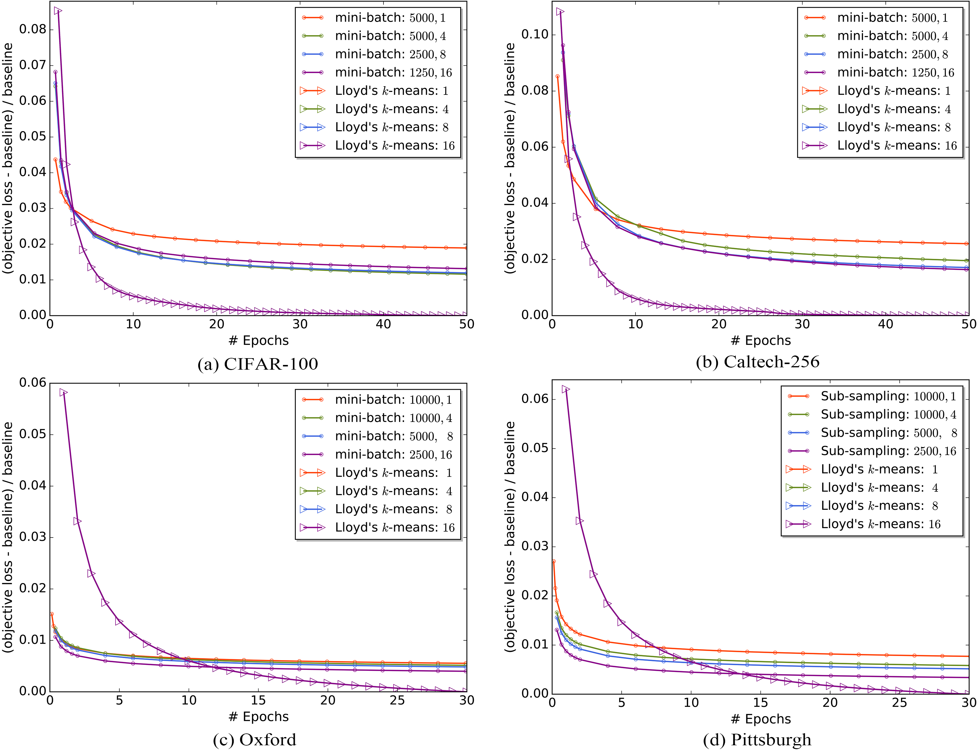
Comparison of convergence performance on four large-scale datasets.

Figure 4.

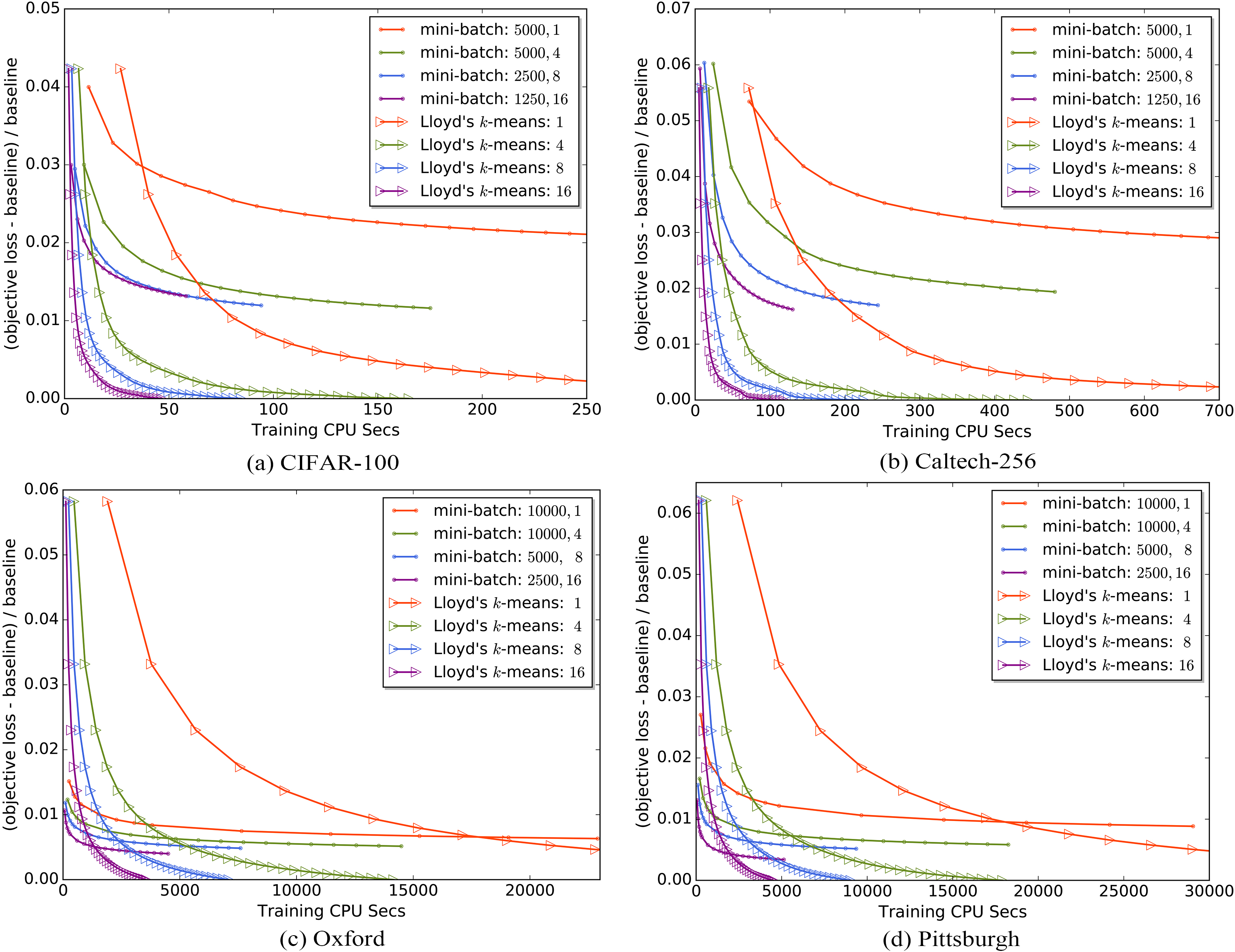
Comparison of speedup on four large-scale datasets.

5.3 Convergence performance

As illustrated in Fig. 3, we conduct the comparison of the objective loss on four datasets. The x-axis represents the number of epochs during the training of the cluster centers. The y-axis represents the decrease of the objective function value against a baseline. We use the last objective function value of Scalable Lloyd’s k-means with one worker as the baseline. All worker number configurations of the two algorithms run 50 epochs on CIFAR-100 and Caltech-256, and 30 epochs on Oxford and Pittsburgh. We vary the iteration number $T$ and the mini-batch size $b$ to ensure different worker number configurations in both algorithms run the same number of epochs on the same dataset. The legend in Fig. 3 shows the mini-batch size $b$ and the worker number $P$ . Note that the four curves with triangular markers overlap completely because Scalable Lloyd’s k-means produces exactly the same result after each epoch, no matter how many workers run the program.

As shown in Fig. 3, Scalable Lloyd’s k-means converges to smaller objective function values than Scalable Mini-Batch k-means, since the latter one induces much stochastic noise. In addition, the final loss value of Scalable Mini-Batch k-means becomes smaller and smaller with the increasing of the worker number $P$ , which benefits from our new aggregation method. As described in Discussion subsection, more workers mean that more different direction update vectors are added to the global parameters in each iteration. Therefore, we can get a more reasonable direction with less stochastic noise. Furthermore, as shown in each subfigure, Scalable Mini-Batch k-means with different worker number configurations consistently converges faster on Oxford and Pittsburgh, but does not show advantage on CIFAR-100 and Caltech-256 compared with Scalable Lloyd’s k-means. The reason may be that when the data size is small, only a few mini batches are used to update cluster centers in each epoch, which is similar to update cluster centers using a full batch in each epoch. In other words, the advantage is more significant on large datasets, which means that Scalable Mini-Batch k-means is efficient to conduct large-scale $k$ -means clustering tasks.

5.4 Speedup

As illustrated in Fig. 4, we conduct the comparison of the clustering speed on four datasets. The experiment setup is the same as that in Fig. 3 except that the x-axis represents CPU seconds. We only show part of the red curve with triangular markers in each subfigure of Fig. 4 due to space constraints.

When we see the curves with the same marker in each subfigure of Fig. 4, we can get very intuitive feeling about the speedup of the two algorithms. The curves with the same marker decrease more steeply and finish earlier with the increase of the workers. To make it more precise, we record the time consumption for the two scalable algorithms with different worker number configurations on four datasets, as illustrated in Table 2. All worker number configurations of the two algorithms run the same epochs as described in the previous subsection. The speedup is the speeding up ratio of different worker number configurations relative to the one worker configuration on the same dataset for each algorithm. First, we can find that the two scalable algorithms both produce almost ideal speedup on every dataset with the increase of the workers. This shows that our algorithms have very good scalability. Especially, Scalable Lloyd’s K-Means even gains super ideal speedup on Oxford and Pittsburgh. The reason is that when the volume of computation in each worker is large enough, more workers may bring more computation benefits than communication overhead incurred by them. Second, generally speaking, the growth rate of the speedup decreases in each algorithm on each dataset when the worker number $P$ increases. This is because more workers incur more communication overhead. Meanwhile, Scalable Mini-Batch k-means always consumes more time on every dataset than Scalable Lloyd’s k-means when the worker number is the same. The reason is that the former one needs two pairs of the push and pull operations every mini-batch, which incurs much more communication overhead than the latter one. However, Scalable Mini-Batch k-means converges faster on large-scale datasets, such as Oxford and Pittsburgh. We do not have to use the same epochs to converge to a reasonable objective loss value and thus we can reduce the time consumption by running less epochs.

Table 2
Comparison of time consumption and speedup on four datasets

Scalable	$P$	CIFAR-100		Caltech-256		Oxford		Pittsburgh
algorithms		Time	Speedup	Time	Speedup	Time	Speedup	Time	Speedup
Scalable	1	672s	1.00 $\times$	1816s	1.00 $\times$	15.83h	1.00 $\times$	20.15h	1.00 $\times$
Lloyd’s	4	168s	4.00 $\times$	454s	4.00 $\times$	3.93h	4.03 $\times$	4.98h	4.05 $\times$
K-means	8	86s	7.81 $\times$	230s	7.90 $\times$	1.97h	8.04 $\times$	2.51h	8.03 $\times$
	16	$\bm{47}$ s	$\bm{14.30}\times$	$\bm{121}$ s	$\bm{15.01}\times$	$\bm{0.99}$ h	$\bm{15.99}\times$	$\bm{1.25}$ h	$\bm{16.12}\times$
Scalable	1	689s	1.00 $\times$	1844s	1.00 $\times$	15.95h	1.00 $\times$	20.17h	1.00 $\times$
Mini-Batch	4	175s	3.94 $\times$	480s	3.84 $\times$	4.03h	3.96 $\times$	5.07h	3.98 $\times$
K-means	8	94s	7.33 $\times$	244s	7.56 $\times$	2.11h	7.56 $\times$	2.60h	7.76 $\times$
	16	$\bm{58}$ s	$\bm{11.88}\times$	$\bm{130}$ s	$\bm{14.18}\times$	$\bm{1.25}$ h	$\bm{12.76}\times$	$\bm{1.42}$ h	$\bm{14.20}\times$

6. Conclusion

We have presented two scalable algorithms for optimizing $k$ -means problem. Both of them can scale beyond computational and memory limits of a single machine based on the data-parallel technique and the parameter server system. The first algorithm can find better quality of solutions, while the second one converges to a modest solution faster. They both have good scalability and totally do in-memory computation. In addition, we propose a new aggregation method for Scalable Mini-Batch k-means. Extensive experiments conducted on four large-scale datasets show that our proposed algorithms have good convergence performance and achieve almost ideal speedup.

Footnotes

Acknowledgments

This work was supported by the National Key R&D Program of China 2018YFB1003203 and the National Natural Science Foundation of China (Grant No. 61672528, 61773392 and 61702539). We thank the National Supercomputing Center in Changsha for providing the Tianhe-1 supercomputer as our experimental platform.

References

Agarwal

P.K.

Har-Peled

and Varadarajan

K.R.

, Geometric approximation via coresets, Combinatorial and Computational Geometry 52 (2005), 1–30.

Bahmani

Moseley

Vattani

Kumar

and Vassilvitskii

, Scalable k-means++, Proc. VLDB Endow 5(7) (Mar. 2012), 622–633.

Bhimani

Leeser

and Mi

, Accelerating k-means clustering with parallel implementations and gpu computing, in: 2015 IEEE High Performance Extreme Computing Conference (HPEC), 2015, pp. 1–6.

Bottesch

Bühler

and Kächele

, Speeding up k-means by approximating euclidean distances via block vectors, in: International Conference on Machine Learning, 2016, pp. 2578–2586.

Bottou

and Bengio

, Convergence properties of the k-means algorithms, in: Advances in Neural Information Processing Systems, 1995, pp. 585–592.

Celebi

M.E.

et al., Partitional clustering algorithms, Springer, 2015.

Chawla

and Gionis

, k-means: A unified approach to clustering and outlier detection, in: Proceedings of the 2013 SIAM International Conference on Data Mining, SIAM, 2013, pp. 189–197.

Dai

Kumar

Wei

Gibson

and Xing

E.P.

, High-performance distributed ml at scale through parameter server consistency models, in: Twenty-Ninth AAAI Conference on Artificial Intelligence, 2015.

Ding

Zhao

Shen

Musuvathi

and Mytkowicz

, Yinyang k-means: A drop-in replacement of the classic k-means with consistent speedup, in: Proceedings of the 32nd International Conference on Machine Learning, 2015, pp. 579–587.

10.

Elkan

, Using the triangle inequality to accelerate k-means, in: Proceedings of the 20th International Conference on Machine Learning, 2003, pp. 147–153.

11.

Griffin

Holub

and Perona

, Caltech-256 object category dataset, 2007.

12.

Hamerly

, Making k-means even faster, in: Proceedings of the 2010 SIAM International Conference on Data Mining, SIAM, 2010, pp. 130–140.

13.

Cipar

Cui

Lee

Kim

J.K.

Gibbons

P.B.

Gibson

G.A.

Ganger

and Xing

E.P.

, More effective distributed ml via a stale synchronous parallel parameter server, in: Advances in Neural Information Processing Systems, 2013, pp. 1223–1231.

14.

Kanungo

Mount

D.M.

Netanyahu

N.S.

Piatko

C.D.

Silverman

and Wu

A.Y.

, An efficient k-means clustering algorithm: Analysis and implementation, IEEE Transactions on Pattern Analysis and Machine Intelligence 24(7) (2002), 881–892.

15.

Krizhevsky

and Hinton

, Learning multiple layers of features from tiny images, 2009.

16.

Wang

and Li

, An efficient k-means clustering algorithm on mapreduce, in: Database Systems for Advanced Applications, Cham, Springer International Publishing, 2014, pp. 357–371.

17.

Newling

and Fleuret

, Fast k-means with accurate bounds, in: International Conference on Machine Learning, 2016, pp. 936–944.

18.

Newling

and Fleuret

, Nested mini-batch k-means, in: Advances in Neural Information Processing Systems, 2016, pp. 1352–1360.

19.

Pelleg

and Moore

, Accelerating exact k-means algorithms with geometric reasoning, in: Proceedings of the Fifth ACM SIGKDD International Conference on Knowledge Discovery and Data Mining, ACM, 1999, pp. 277–281.

20.

Perd’och

Chum

and Matas

, Efficient representation of local geometry for large scale object retrieval, in: IEEE Conference on Computer Vision and Pattern Recognition, IEEE, 2009, pp. 9–16.

21.

Philbin

Chum

Isard

Sivic

and Zisserman

, Object retrieval with large vocabularies and fast spatial matching, in: IEEE Conference on Computer Vision and Pattern Recognition, IEEE, 2007, pp. 1–8.

22.

Sculley

, Web-scale k-means clustering, in: Proceedings of the 19th International Conference on World Wide Web, ACM, 2010, pp. 1177–1178.

23.

Simonyan

and Zisserman

, Very deep convolutional networks for large-scale image recognition, arXiv preprint arXiv:1409.1556, 2014.

24.

Sreedhar

Kasiviswanath

and Reddy

P.C.

. Clustering large datasets using k-means modified inter and intra clustering (km-i2c) in hadoop, Journal of Big Data 4(1) (2017), 1–19.

25.

Steinbach

Karypis

Kumar

et al., A comparison of document clustering techniques, in: KDD Workshop on Text Mining, Boston, Vol. 400, 2000, pp. 525–526.

26.

Torii

Sivic

Okutomi

and Pajdla

, Visual place recognition with repetitive structures, IEEE Transactions on Pattern Analysis and Machine Intelligence 37(11) (2015), 2346–2359.

27.

Xing

E.P.

Dai

Kim

J.K.

Wei

Lee

Zheng

Xie

Kumar

and Yu

, Petuum: A new platform for distributed machine learning on big data, IEEE Transactions on Big Data 1(2) (2015), 49–67.

28.

Zhang

and Hao

, A parallel k-means clustering algorithm with mpi, in: 2011 Fourth International Symposium on Parallel Architectures, Algorithms and Programming, 2011, pp. 60–64.

Scalable k -means for large-scale clustering

Abstract

Keywords

1. Introduction

2. Related work

3. Preliminaries

3.1 K-means clustering

4.1 Scalable Lloyd’s k-means

4.2 Scalable Mini-Batch k-means

4.3 Discussion

5. Experiments

5.1 Datasets and environment

Table 1 Summary of the datasets

5.4 Speedup

Table 2 Comparison of time consumption and speedup on four datasets

Footnotes

Acknowledgments

References

Table 1
Summary of the datasets

Table 2
Comparison of time consumption and speedup on four datasets