Bayesian optimization of support vector machine for regression prediction of short-term traffic flow

Abstract

Short-term traffic flow prediction plays a crucial component in transportation management and deployment. In this paper, a novel regression framework for short-term traffic flow prediction with automatic parameter tuning is proposed, with the SVR being the primary regression model for traffic flow prediction and the Bayesian Optimization being the major method for parameters selection. First, the preprocessing of raw traffic flow is carried out by seasonal difference to eliminate the non-stationary of the data. Then, Support Vector Regression model is trained by the pre-processed data. In order to optimize the model parameters, the generalization performance of SVR is modeled as a sample from a Gaussian process (GP). Bayesian optimization determines the parameters configuration of the regression model by optimizing the acquisition function over the GP. Finally, the optimal short-term traffic flow regression model is constructed through repeated GP update and iteratively multiple training of the model. Experiment results show that the accuracy of proposed method is superior to methods of classical SARIMA, MLP-NN, ERT and Adaboost.

Keywords

Short-term traffic flow prediction bayesian optimization gaussian process support vector regression

1. Introduction

With the economic development and people’s increasing demand for convenient transportation, the vehicles have been experienced fast-growth in recent years, which brings tremendous traffic pressure for limited road resources. Accurate traffic flow prediction could estimate the congestion level of the road, therefore leading the driver to choose the best route to reach the destination and providing more effective guidance to traffic authorities[22]. Among the numerous branches of Intelligent Transportation System (ITS), short-term traffic flow prediction plays a fundamental role and is also a challenging task to be calculated due to a lot of influencing factors. Therefore, short-term traffic flow forecast in recent decades has attracted the attention of many researchers.

Through the mining and learning of the changing trend of traffic flow, and combing the current traffic flow data to predict the future traffic flow, a traffic flow forecast model is constructed. Formally, given a traffic flow time sequence $\left\{X_{1},\ldots,X_{t}\right\}$ and some observed vehicle information (such as speed or lane occupancy) at a major road node, the goal for traffic forecasting is to predict the traffic flow ${X_{t}}+\Delta$ at the moment $t+\Delta$ [9]. There is no clear definition of short-term traffic flow. In general, $\Delta$ is less than fifteen minutes. Through statistical analysis, it can be concluded that fifteen minutes is enough for the management system and drivers to make a response to the current road conditions.

Since traffic flow prediction is a nonlinear regression problem, the value of the predicted target is not a simple linear relationship with the existing data. To resolve this, in this paper, we choose SVR as basic method for predicting traffic flow. Through the kernel function, the low-dimensional traffic flow data can be transformed into high-dimensional space, and then the regression prediction problem is transformed into a convex quadratic programming problem by constructing a linear decision-making function. SVR could reach the global optimal solution by employing structural risk minimization principle, so that it can avoid falling into the local maximum. As the same with the almost all machine learning algorithms, they are rarely parameter-free. The parameters determine the generalization ability of the underlying SVR model. However, parameter tuning is often a “black art” requiring expert experience, rules of thumb, or sometimes bruteforce search[16]. Nearly all machine learning methods that are used to predict traffic flow have not proposed an effective method to solve the problem of parameters adjustment, which makes the model almost impossible to achieve the optimal effect. Thus, this restricts the development of machine learning algorithms in the field of traffic flow forecasting.

Therefore, in this paper, we propose a new framework, called BO-SVR, for short-term traffic flow forecasting. First, The idea of SARIMA is used to process the traffic flow data to ensure the stationary. Then SVR is selected as basic regression method, data related to traffic flow at preceding periods is considered as input, and traffic volumes at current period are considered as output. The RBF kernel function is used in this SVR model. There are three parameters in SVR: the penalty parameter $C$ , non-sensitive loss parameter $\varepsilon$ and the kernel parameter $\sigma$ . The parameters dominate the learning efficiency and the capacity of the underlying model. Different from the previous methods, this paper chooses Bayesian optimization method to select optimal parameters $\left({C,\varepsilon,\sigma}\right)$ by viewing the process of optimizing the model as the maximization of an unknown function.

The remainder of this paper is organized as follows. Section 2 is related work. Section 3 introduces support vector regression, which is preliminaries for later sections. Section 4 describes the details of the Bayesian optimization based SVR model. Then, experimental process and experimental results which compared with other mainstream methods are presented in Section 5. Finally, some conclusions and directions for the future works are given in Section 6.

2. Related work

A wide variety of approaches have been proposed for short-term traffic flow forecasting. From the view of spatio-temporal algorithms, the modeling and prediction of traffic flow are based on the probabilistic graph perspective. There are some methods like Markov chains[23], Markov random fields (MRFs) and Kalman filters[13, 21] which have shown the best experimental results. In contrast with the spatio-temporal methods, single-location prediction model is easy to acquire and it is more practical. Therefore, in this paper, we focus on the study on accurately and efficiently predicting traffic flow at single locations. For single-location traffic flow prediction, classical time-series approaches have played an important role. Box and Jenkins[1] are important contributors to this field. They put forward autoregressive moving average (ARMA) algorithm that has achieved reasonable results in traffic flow prediction. Since then, enhanced versions of ARMA, such as ARIMA, seasonal ARIMA, are widely used in traffic flow forecasting. These models can capture the dynamics of linear system well. However, traffic flow forecasting is a non-linear problem, these models are unable to achieve the best predictive results for traffic flow prediction. Research shows that machine learning methods usually have better ability to capture the uncertainty and complex nonlinearity of traffic flow time series. There are three commonly used methods: support vector regression (SVR)[17], artificial neural networks (ANNs)[11] and Bayesian networks[18]. Recently, deep learning has also drawn a lot of academic and industrial interests[10]. For almost all machine learning algorithms, careful tuning of parameters is inevitable. The failure to choose the optimal parameters has become an important factor hindering the performance improvement of the algorithm.

In order to maximize the rate of learning and the capacity of the underlying model, in recent years, some experts have put forward automated method to optimize parameters of machine learning. Specifically, we could regard the process of parameters adjustment as the maximization of a black-box function[16], regard parameters of the model as independent variables of the function, and regard the generalization ability of the model as dependent variables of the function. Through the optimization method to obtain the maximum value of the function, a set of optimal parameters are obtained. For this reason, the traffic flow forecasting model based on the machine learning method can achieve the best learning performance. There are many function optimization methods, such as gradient optimization methods or Monte Carlo sampling methods. However, there is no specific expression for the function that needs to be optimized in this paper. The particle swarm optimization (PSO) algorithm may fall into the local optimal solution[15]. A good choice is Bayesian optimization[12], which has been shown to outperform other state of the art global optimization algorithms on a number of challenging optimization functions[5]. Jasper et al.[16] also proved the application of Bayesian optimization in machine learning achieved good results by theory and experiment.

3. Support vector regression model

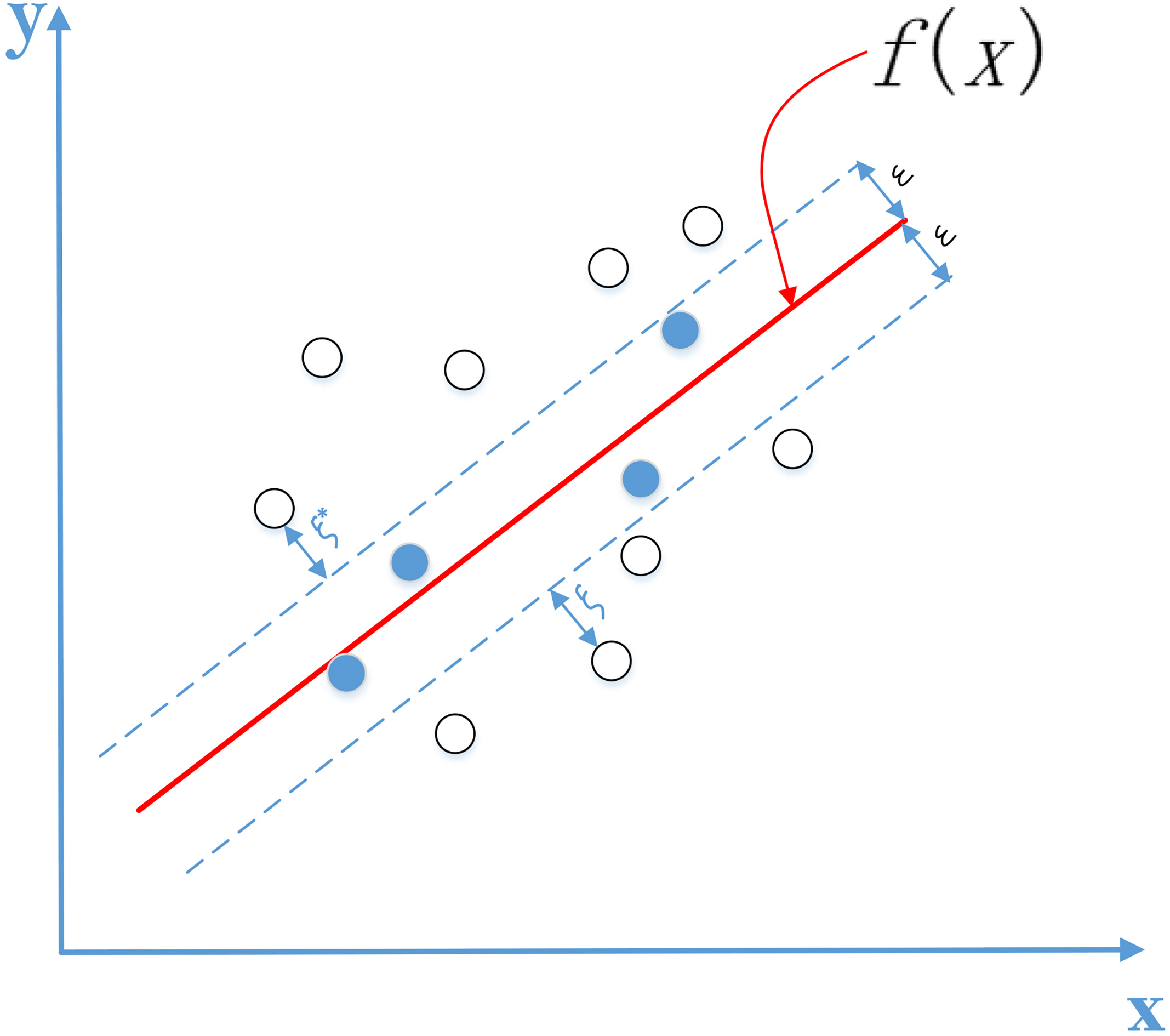
Traffic flow at a fixed point is influenced by many factors and has great variability. The prediction of traffic flow is quite complex, which is a typical nonlinear time series forecasting problem. There are many nonlinear prediction methods which are presented for time series prediction. Support Vector Regression (SVR) based methods are one of the widely applied methods and can achieve satisfactory results in predicting small sample high dimensional data, nonlinear problem and local minima problem, etc.[4]. SVR as a machine learning method was firstly proposed in 1996 by Drucker et al.[3]. It is based on the statistical learning theory and has strict mathematical basis, which enhances the generalization ability by employing structural risk minimization principle and provides better predictions to many practical problems[4].

For a given traffic flow training data $D=\{({x_{1}},{y_{1}}),({x_{2}},{y_{2}}),\ldots,({x_{n}},{y_{n}})\},{x_{i}},{y_% {i}}\in R$ , each $x_{i}$ denotes the feature vector of the sample and has a corresponding target value of traffic flow $y_{i}$ for $i=1,2,\ldots,n$ . The Support Vector Regression (SVR)’s basic idea is to construct a nonlinear map from input space to output space and map the input data to a higher dimensional feature space through kernel function. A regression function model, as shown below, is wished to be learned through training.

$\displaystyle f(x)=\omega\cdot\varphi(x)+b$ (1)

where $\varphi(x)$ denotes a nonlinear function in which the input data $x$ is transformed into a high dimensional feature space. Therefore, the nonlinear problem of low dimension transforms into the linear problem of high dimension. $\omega$ contains the coefficients that have to be estimated by training data, and $b$ is a real constant that should also be learned. The objective of SVR can be formulated by the expression below.

$\displaystyle\mathop{\min}\limits_{\omega,b,{\xi_{i}},\xi_{i}^{*}}\frac{1}{2}{% \left\|\omega\right\|^{2}}+C\sum\limits_{i=1}^{n}{({\xi_{i}}+\xi_{i}^{*})}$ (2)

$\displaystyle s.t\left\{{\begin{array}[]{l}{f{{(x)}_{i}}-{y_{i}}\leqslant% \varepsilon+{\xi_{i}}}\\ {{{{y}}_{i}}-f({x_{i}})\leqslant\varepsilon+\xi_{i}^{*}}\\ {{\xi_{i}}\geqslant 0,\xi_{i}^{*}\geqslant 0,i=1,2,\ldots,n.}\end{array}}\right.$ (3)

where ${\xi_{i}}$ is the lower slack variable ( ${\xi_{i}^{*}}$ is the upper) subjecting to the $\varepsilon$ -insensitive tube $y-f(x)\leqslant\varepsilon$ , the first term $1/2{\left\|\omega\right\|^{2}}$ is called the regularization term which can improve generalization of model. The second item is experiential error. Parameter $C$ is the regularization constant that determines the trade-off between believing risk and experiential error.

In Eq. (3), the non-sensitive loss parameter $\varepsilon$ is usually a positive constant. The constraints of Eq. (2) imply that if the difference between the predictive value $f({x_{i}})$ and the real value ${y_{i}}$ is less than $\varepsilon$ , the loss is ignored. That is to say, as shown in the Fig. 1, the real value ${y_{i}}$ of the data ${x_{i}}$ is placed inside the tube $\varepsilon$ , the error is zero. If ${y_{i}}$ is outside the tube, the error is ${\xi_{i}}$ or $\xi_{i}^{*}$ . To avoid underfitting and overfitting of the training data, the regularization term $1/2{\left\|\omega\right\|^{2}}$ as well as the training error $C\sum_{i=1}^{n}{({\xi_{i}}+\xi_{i}^{*})}$ should be minimized[19].

Figure 1.

$\varepsilon$ -insensitive tube for SVR.

In order to minimize Eq. (2), introducing Lagrange multipliers, and the Lagrange function can be obtained as follows:

$\displaystyle L(\omega,b,\alpha,{\alpha^{*}},\xi,{\xi^{*}},\mu,{\mu^{*}})=% \frac{1}{2}{\left\|\omega\right\|^{2}}+C\sum\limits_{i=1}^{n}{\left({{\xi_{i}}% +\xi_{i}^{*}}\right)-}\sum\limits_{i=1}^{n}{{\mu_{i}}}{\xi_{i}}$ (4) $\displaystyle\quad-\sum\limits_{i=1}^{n}{\mu_{i}^{*}\xi_{i}^{*}}+\sum\limits_{% i=1}^{n}{{\alpha_{i}}\left({f\left({{x_{i}}}\right)-{y_{i}}-\varepsilon-{\xi_{% i}}}\right)}+\sum\limits_{i=1}^{n}{\alpha_{i}^{*}\left({{y_{i}}-f\left({{x_{i}% }}\right)-\varepsilon-\xi_{i}^{*}}\right)}$

then, calculate the partial derivatives of the four independent variables $\left({\omega,b,\xi,{\xi^{*}}}\right)$ and let the partial derivative be zero,and we can get:

$\displaystyle\omega=\sum\limits_{i=1}^{n}{\left({\alpha_{i}^{*}-{\alpha_{i}}}% \right)}$ (5) $\displaystyle{{0}}=\sum\limits_{i=1}^{n}{\left({\alpha_{i}^{*}-{\alpha_{i}}}% \right)}$ (6) $\displaystyle C={\alpha_{i}}+{\mu_{i}}$ (7) $\displaystyle C=\alpha_{i}^{*}+\mu_{i}^{*}$ (8)

substituting the above Eqs (5)–(8) into Eq. (3), the problem of Eq. (2) can be transformed into the following dual problem, which is a convex quadratic problem.

$\displaystyle\mathop{\max}\limits_{\alpha,{\alpha^{*}}}\left\{{\begin{array}[]% {l}{-\frac{1}{2}\sum\limits_{i,j=1}^{n}{\left({\alpha_{i}^{*}-{\alpha_{i}}}% \right)\left({\alpha_{j}^{*}-{\alpha_{j}}}\right)K\left({{x_{i}},{x_{j}}}% \right)}}\\ {-\varepsilon\sum\limits_{i=1}^{n}{\left({\alpha_{i}^{*}+{\alpha_{i}}}\right)+% \sum\limits_{i=1}^{n}{{y_{i}}\left({\alpha_{i}^{*}-{\alpha_{i}}}\right)}}}\end% {array}}\right.$ (9)

$\displaystyle s.t\left\{{\begin{array}[]{l}{\sum\limits_{i=1}^{n}{\left({% \alpha_{i}^{*}-{\alpha_{i}}}\right)=0}}\\ {0\leqslant{\alpha_{i}},\alpha_{i}^{*}\leqslant C}\end{array}}\right.$ (10)

The above process is constrained by KKT optimality conditions:

$\displaystyle\left\{{\begin{array}[]{l}{{\alpha_{i}}\left({f\left({{x_{i}}}% \right)-{y_{i}}-\varepsilon-{\xi_{i}}}\right)={{0}}}\\ {\alpha_{i}^{*}\left({{y_{i}}-f\left({{x_{i}}}\right)-\varepsilon-\xi_{i}^{*}}% \right)={{0}}}\\ {{\alpha_{i}}\alpha_{i}^{*}=0,{\xi_{i}}\xi_{i}^{*}=0,}\\ {\left({C-{\alpha_{i}}}\right){\xi_{i}}=0,\left({C-\alpha_{i}^{*}}\right)\xi_{% i}^{*}=0.}\end{array}}\right.$ (11)

Finally, the regression result can be expressed as:

$\displaystyle\mathop{f}\limits^{\wedge}(x)=\sum\limits_{i=1}^{n}{(\alpha_{i}^{% *}-{\alpha_{i}})}K({x_{i}},x)+b$ (12)

where $K\left({{x_{i}},x}\right)$ is kernel function. Since the traffic flow forecasting is not a linear regression problem, by using the kernel function, we can map data of low-dimensional space to a high-dimensional space so that it can be linear regression. The typical kernel functions are linear, polynomial, and Gaussian, etc. Choosing a suitable kernel function is crucial to SVR algorithm. We use the RBF kernel function in this paper, as shown in Eq. (13).

$\displaystyle K\left({{x_{i}},{x_{j}}}\right)=\exp\left({-\frac{{{{\left\|{{x_% {i}}-{x_{j}}}\right\|}^{2}}}}{{2{\sigma^{2}}}}}\right)$ (13)

here, $\sigma$ is kernel parameter gamma, which influences the performance of SVR models seriously. So, parameter gamma also should be chosen correctly.

4. Proposed method

In training the SVR model, the traffic flow data collected in the past is used as input value, and the traffic flow at the current moment is regarded as the output value. For parameter settings, in traditional support vector regression, it is usually manual tuning that can not achieve best results. To improve this, we propose an efficient Bayesian optimization based method that selects parameters automatically.

4.1 Bayesian optimization

Bayesian optimization is an effective method for finding the extrema of objective function that does not have a closed-form expression, but can obtain observations by sampling. What makes Bayesian optimization different from other approaches is that it constructs a probabilistic model for objective function $f(x)$ , and by sampling the objective function, a prior distribution can be obtained. The prior represents our belief about the objective functions. Through the Bayesian theory, the posterior distribution of the objective function can be calculated, which captures our updated beliefs about the unknown objective function. And then we exploit this model to determine the next point to evaluate in some bounded set $X$ . By making full use of information available from previous evaluations of $f(x)$ but not simply rely on local gradient and Hessian approximations, Bayesian optimization can find the maximum of complex non-convex functions with relatively few evaluations.

There are two major parts that must be discussed when introducing Bayesian optimization. First, prior distribution expresses assumptions about the function being optimized, so it must be discussed in detail. Because of the flexibility and tractability of the Gaussian process prior, here we choose it as prior over functions. The second point is acquisition function, which is used to construct a utility function to determine the next point to evaluate. Next, we will review the Gaussian process prior and acquisition function. For a detailed overview of the Bayesian optimization formalism, see, e.g., Brochu et al.[2].

4.1.1 Gaussian process

Gaussian process (GP) offers a convenient and powerful prior distribution over the space of smooth functions. A Gaussian process is a set of infinite number of random variables, where any finite number of random variables are subject to a joint Gaussian distribution[14]. The sampling points on an unknown function can be treated as random variables of GP, so it can be assumed that the function conforms to the Gaussian process. The formula is expressed as follows:

$\displaystyle f(x)\sim GP(\mu(x),k(x,{x^{*}}))$ (14)

The support and properties of Gaussian process are determined by its mean function $\mu\left(x\right)$ and covariance function $k\left({x,{x^{*}}}\right)$ . By selecting some of the sampling points of the unknown function as priori, we assumed that these points are part of the GP. That is to say, they are subject to multivariate Gaussian distributions. By using the properties of the multivariate Gaussian distribution, the mean and variance can be calculated. Usually in the Gaussian process, the priori mean function can be assumed to be zero and without any loss of generality. This leaves the Gaussian process completely determined by the covariance functions. The power of the Gaussian process to express information on the objective function depends entirely on covariance function. In particular, squared exponential covariance function

$\displaystyle k\left({x,{x^{*}}}\right)=\exp\left({-\frac{1}{2}{{\left\|{x-{x^% {*}}}\right\|}^{2}}}\right)$ (15)

is a popular choice for Gaussian process. MatÃ©rn kernel is another popular choice of the covariance function[6].

Let’s initialize the sample points from the objective function. We would get $\left\{{{x_{1}},{x_{2}},\ldots,{x_{t}}}\right\}$ and the corresponding function values $\left\{{{y_{1}},{y_{2}},\ldots,{y_{t}}}\right\}$ , where ${y_{1:t}}=f\left({{x_{1:t}}}\right)$ . One could view that these data pairs $\left\{{{x_{1:t}},{y_{1:t}}}\right\}$ are sampled from the prior Gaussian process with its mean value being zero and the covariance function $k\left({{x_{i}},{x_{j}}}\right)$ . The function values ${y_{1:t}}$ thus follow a joint Gaussian distribution $N\left({0,K}\right)$ , and the covariance matrix is given by:

$\displaystyle K=\left[{\begin{array}[]{ccc}{k\left({{x_{1}},{x_{1}}}\right)}&% \cdots&{k\left({{x_{1}},{x_{t}}}\right)}\\ \vdots&\ddots&\vdots\\ {k\left({{x_{t}},{x_{1}}}\right)}&\cdots&{k\left({{x_{t}},{x_{t}}}\right)}\end% {array}}\right]$ (16)

where the diagonal values are 1 and this matrix is the positive definite matrix. Note that we are considering in a noise-free environment. Also, recall that we have chosen the zero-mean function for simplicity.

In each iteration of our optimization task, we use the sampled data to fit the GP and obtain a posterior distribution from an external model. For each iteration we use acquisition function combining the posterior distribution to decide what point ${x_{t+1}}$ should be evaluated next. It has been proved that optimal optimization results can be obtained by using as little iteration as possible[8]. For this arbitrary point, let us denote the value of the function as ${y_{t+1}}=f\left({{x_{t+1}}}\right)$ . Likewise, ${y_{1:t}}$ and ${y_{t+1}}$ also subject to a joint Gaussian distribution, by the properties of Gaussian processes we could get:

$\displaystyle\left[{\begin{array}[]{c}{{y_{1:t}}}\\ {{y_{t+1}}}\end{array}}\right]\sim N\left({0,\left[{\begin{array}[]{cc}K&{\rm{% k}}\\ {{{\rm{k}}^{T}}}&{k\left({{x_{p+1}},{x_{p+1}}}\right)}\end{array}}\right]}\right)$ (17)

where ${\rm{k}}=\left[{k\left({{x_{1}},{x_{t+1}}}\right)k\left({{x_{2}},{x_{t+2}}}% \right)\ldots k\left({{x_{t}},{x_{t+1}}}\right)}\right]$ . Using the Sherman-Morrison-Woodbury formula [14], the posterior distribution of the objective function can be written as:

$\displaystyle P\left({{y_{t+1}}|{x_{1:t}},{y_{1:t}}}\right)\sim N\left({{\mu_{% t}}\left({{x_{t+1}}}\right),\sigma_{t}^{2}\left({{x_{t+1}}}\right)}\right)$ (18)

where

$\displaystyle{\mu_{t}}\left({{x_{t+1}}}\right)={{\rm{k}}^{T}}{K^{-1}}{y_{1:t}}$ (19) $\displaystyle\sigma_{t}^{2}\left({{x_{t+1}}}\right)=k\left({{x_{t+1}},{x_{t+1}% }}\right)-{{\rm{k}}^{\rm{T}}}{K^{-1}}{\rm{k}}.$ (20)

So far, we have discussed the Gaussian process priors over the objective function, and how to update these prior knowledges according to the new observation.

4.1.2 Acquisition function

As mentioned earlier, the acquisition function is used to determine the next point to evaluate, thus it guides the search to the optimum. In Bayesian optimization, the acquisition function could be viewed as a surrogate function, which is easy to evaluate, to optimize the expensive functions. Typically, the high value of the acquisition function corresponds to the potential maximum of the objective function. Because the high acquisition represents the prediction of the objective function is high or the uncertainty is great. Maximizing the acquisition function is used to determine the next point at which to evaluate the objective function. That is, we wish to sample $f$ at ${{argma}}{{\rm{x}}_{x}}u\left({x|D}\right)$ , where $u\left(\cdot\right)$ is the generic symbol of acquisition function.

There are several popular choices of acquisition function, which either using improvement based criteria or using confidence based criteria. The following are introduced separately. In the following, $\varphi\left(\cdot\right)$ and $\Phi\left(\cdot\right)$ represent the PDF and CDF of the standard normal distribution respectively. ${x_{\textit{best}}}=\arg{\max_{{x_{i}}\in{x_{1:t}}}}f\left({{x_{i}}}\right)$ denotes the current best observation. $\mu\left(x\right)$ and $\sigma\left(x\right)$ indicate the predictive mean function and predictive variance function of the objective function respectively.

Probability of Improvement(PI)

$\displaystyle{a_{PI}}\left(x\right)=\Phi\left({\gamma\left(x\right)}\right),% \gamma\left(x\right)=\frac{{f\left({{x_{best}}}\right)-\mu\left(x\right)}}{{% \sigma\left(x\right)}}$ (21)

The strategy of PI is to maximize the probability of improving over the best current value[7]. The attendant drawback is that this formulation is pure exploitation without exploration. As a result, an alternative acquisition function is Expected Improvement(EI), which chooses to maximize the expected improvement over the current best.

Expected Improvement(EI)

$\displaystyle a_{\textit{EI}}(x)=\left\{\begin{array}[]{cc}(\mu(x)-f(x_{% \textit{best}}))\Phi(\gamma(x))+\sigma(x)\varphi(x)&\textit{if}\ \sigma\left(x% \right)>0\\ 0&\textit{if}\ \sigma\left(x\right)=0\end{array}\right.$ (22)

Another acquisition function is GP-UCB[19], which uses the upper confidence bound of the GP predictive distribution.

GP Upper Confidence Bound(GP-UCB)

$\displaystyle a_{\textit{UCP}}=\mu\left(x\right)+k\sigma\left(x\right)$ (23)

where $k$ is used to balance exploitation against exploration.

In this paper, we will focus on the EI criterion, as it has been shown to be better-behaved than PI, but unlike GP-UCP, it does not require its own tuning parameter. In each iteration, we use the acquisition function to determine whether to exploit or to explore in next sampling. Eventually, the global maximum of the objective function can be obtained instead of the local maximum.

4.2 Support vector regression prediction based on bayesian optimization

As mentioned above, it is difficult to achieve optimal learning results by manually adjusting the SVR parameters. To improve this, therefore, we propose an effective support vector regression approach based on Bayesian optimization (BO-SVR) for short-term traffic flow prediction.

In the section II, SVR is introduced, which has three tuning parameters $\left({{\rm{C}},\varepsilon,\sigma}\right)$ . The penalty coefficient $C$ reflects the degree of penalty for the sample data beyond the pipe $\varepsilon$ , and its value affects the complexity and stability of the model. The insensitive loss coefficient $\varepsilon$ controls the width of the regression function’s insensitive region of the sample data. $C$ and $\varepsilon$ determine the learning accuracy and generalization of this model. $\sigma$ is kernel parameter gamma. The larger the $\sigma$ value, the smaller the structural risk, the smoother the function curve, but the greater experiential risk. If the value of $\sigma$ becomes smaller, the situation changes to the opposite. Thus, if the appropriate $\left({{\rm{C}},\varepsilon,\sigma}\right)$ combination can be selected, the exact and stable regression model can be obtained.

In order to optimize these parameters automatically, we could view such tuning as the optimization of an unknown black-box function $f\left(x\right)$ . Specifically, we view such parameters $\left({{\rm{C}},\varepsilon,\sigma}\right)$ as independent variables of the function, and view the generalization ability of SVR as dependent variables of the function. Here, the prediction accuracy $\left(m\right)$ of traffic flow is regarded as a representation of generalization. Now, the objective function has been defined and satisfies Bayesian optimization conditions. Combined with Gaussian process and the acquisition function, the optimal combination of parameters can be found after several iterations, thus the short-term traffic flow prediction modeled by SVR can be optimized. The detailed steps of the proposed BO-SVR method are shown in pseudocode as Algorithm 1.

[h] .BO-SVR Algorithm[1] Input: The initial observation ${\rm{D}}=\left\{{{x_{1:p}},{m_{1:p}}}\right\}$ , where $x=\left({C,\varepsilon,\sigma}\right)$ . Initial Settings: Establish training data set $T r$ , testing data set $T e$ . Output: $\left\{{x_{t}^{*},m_{t}^{*}}\right\}_{t=1}^{T}$ . t = 1; 2;…T Find ${x_{t}}$ by optimizing the acquisition function over the GP: $x_{t}^{*}=\arg{\max_{x}}a\left({x|D}\right)$ . Re-training SVR model with parameter $x_{t}^{*}=\left({{C_{t}},{\varepsilon_{t}},{\sigma_{t}}}\right)$ on training set $T r$ . Testing the SVR model on the test set $T e$ , obtain the accuracy $m_{t}^{*}$ . Augment the observation set $D=D\cup\left({x_{t}^{*},m_{t}^{*}}\right)$ and update the GP.

Figure 2.

Traffic flow collection sites selected.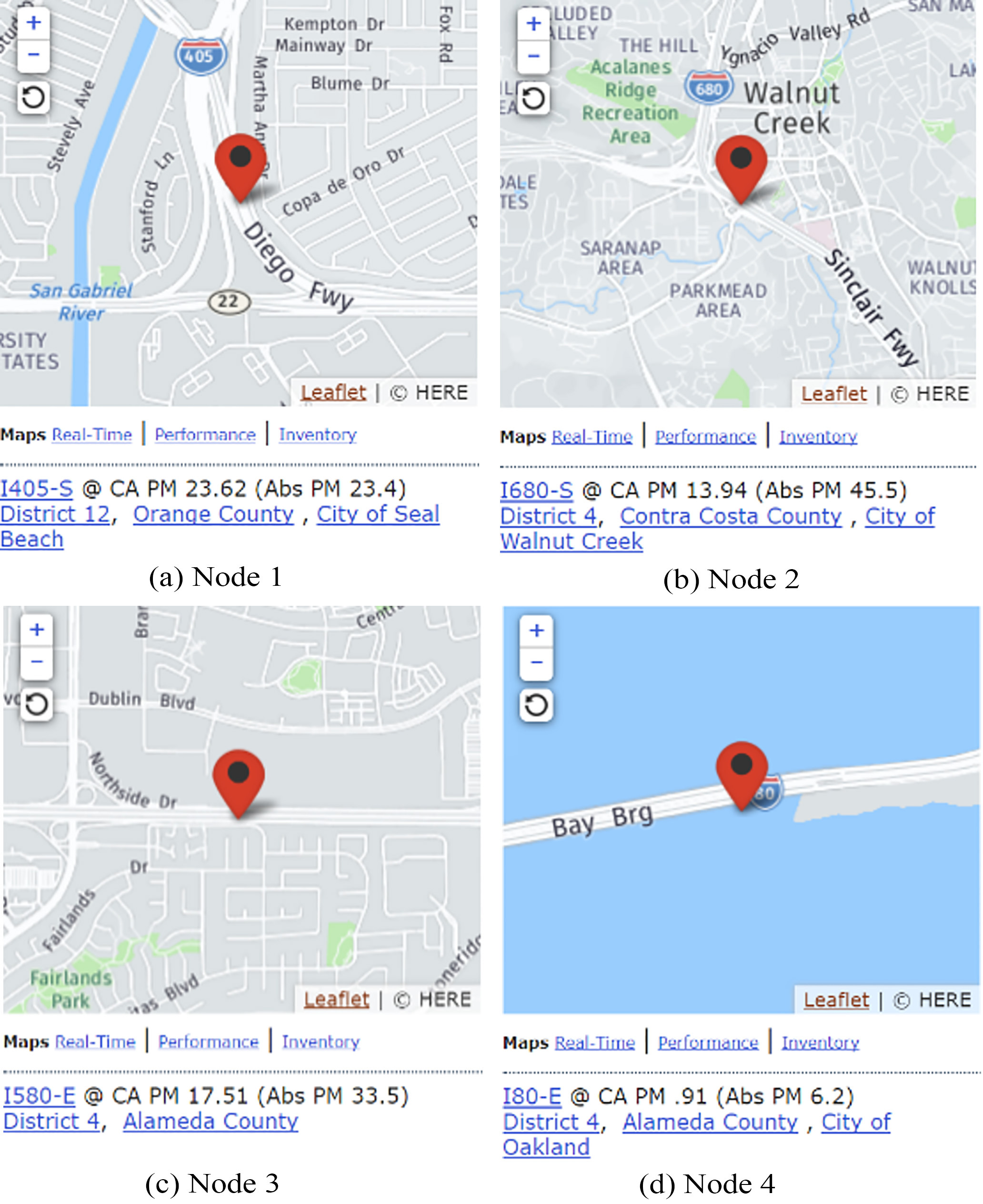

5. Experiment

5.1 Experimental settings

Data Sets:The data we used for traffic flow prediction is downloaded from Caltrans Performance Measurement System (PeMS) public database, which is the most widely used data set in traffic flow prediction. There are over 15000 individual detectors located all over the state in the freeway system of California. The data is collected every 30 seconds from these detectors. Then, the data is aggregated as counts of cars into 5-min periods and is uploaded to the Internet for researcher to use. In our experiment, we further aggregate the data into 15-min periods. Then, we select 4 typical detectors for study since roads in these cases attract more attention for transportation research. As shown in Fig. 2, Node 1 is a busy road section with larger traffic flow. Node 2 is selected, for its location being near cross roads. Node 3 is the main road, and Node 4 is on the bridge.

The time range selected is from 2017-9-25 to 2017-10-9,from 2017-6-25 to 2016-7-9 and from 2017-9-25 to 2017-10-9. We use the data of the first 2 weeks as the training set and the remaining data as the testing set, mainly used for predicting two peak periods flow including 5:00–10:00 AM and 5:00–10:00 PM, the predicted intervals are 5 minutes and 15 minutes. Inspired by the SARIMA model[20], we perform the following pre-processing in order to ensure the stationary (For detailed explanation, please refer to Appendix) of the data. Denoting ${v_{i}}$ as traffic flow at time index $i$ and there are week time indexes in one week, and day time indexes in one day, the data set is constructed as:

$\displaystyle\{\left({X,y}\right)|X=[v_{i-1},v_{i-1}-v_{i-2},v_{i-\textit{week% }},v_{i-\textit{week}}-v_{i-\textit{week}-1},v_{i-\textit{day}},v_{i-\textit{% day}}-v_{i-\textit{day}-1}]^{T},y={v_{i}}\}$ (24)

Evaluation metrics: Performance of time series forecasting is typically using error measures. To evaluate the effectiveness of our proposed model, we use three performance indexes, which are mean absolute percentage error (MAPE), root mean square error (RMSE), mean absolute error (MAE). MAPE is a measure of prediction accuracy of a forecasting method. It usually expresses accuracy as a percentage, and we can get the prediction accuracy(m) by $m=1-\textit{MAPE}$ , which is also the optimization objective of Bayesian Optimization in our model. The concept of MAPE is very intelligible and convincing, but the drawback is that it will cause serious distortion when the observation value is equal to zero or close to zero. Therefore, RMSE and MAE are chosen to measure the performance of the model in this paper. RMSE is the square root of the average of squared errors. The effect of each error on RMSE is proportional to the size of the squared error, thus, larger error has a disproportionately large effect on RMSE. Consequently, RMSE is sensitive to outliers. MAE is relatively simple, which is mainly used to calculate the absolute average error of the prediction model. These indexes are formulated as:

$\displaystyle\textit{MAPE}=\frac{1}{n}\sum\limits_{i=1}^{n}{\frac{{\left|{{f_{% i}}-f_{i}^{*}}\right|}}{{{f_{i}}}}}\times 100$ (25) $\displaystyle\textit{RMSE}=\sqrt{\frac{1}{n}\sum\limits_{i=1}^{n}{{{\left({% \left|{{f_{i}}-f_{i}^{*}}\right|}\right)}^{2}}}}$ (26) $\displaystyle\textit{MAE}=\frac{1}{n}\sum\limits_{i=1}^{n}{\left|{{f_{i}}-f_{i% }^{*}}\right|}$ (27)

where ${f_{i}}$ is the observation value of traffic flow, $f_{i}^{*}$ is the predictive value of traffic flow, and is the total number of observations.

Experimental Design: The performance of the proposed traffic flow forecast method (BO-SVR) is examined with two parts. The first set of experiments is designed to verify the effectiveness of Bayesian Optimization for parameter selection of traffic flow method based on support vector regression. The second group will compare to other classical traffic flow prediction methods, with aim of verifing the overall effectiveness of our proposed method.

Figure 3.

Performance comparison of using default parameters and using parameters selected by Bayesian optimization.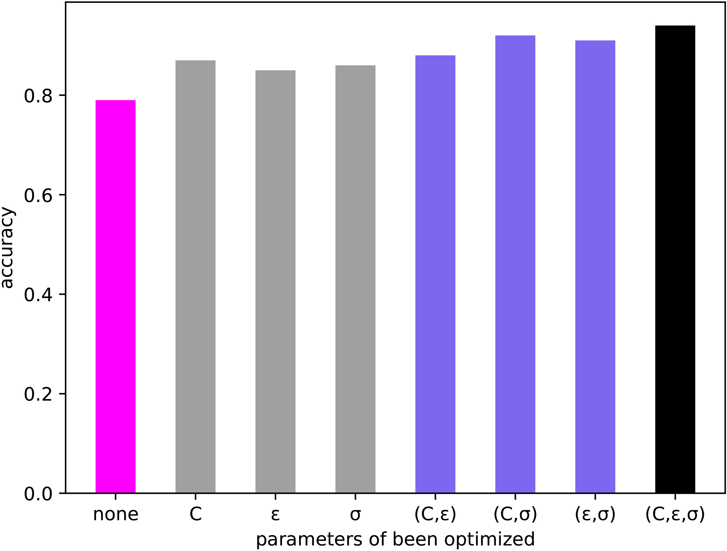

Figure 4.

Prediction of the traffic flow and that of the real traffic flow in one day on node 3.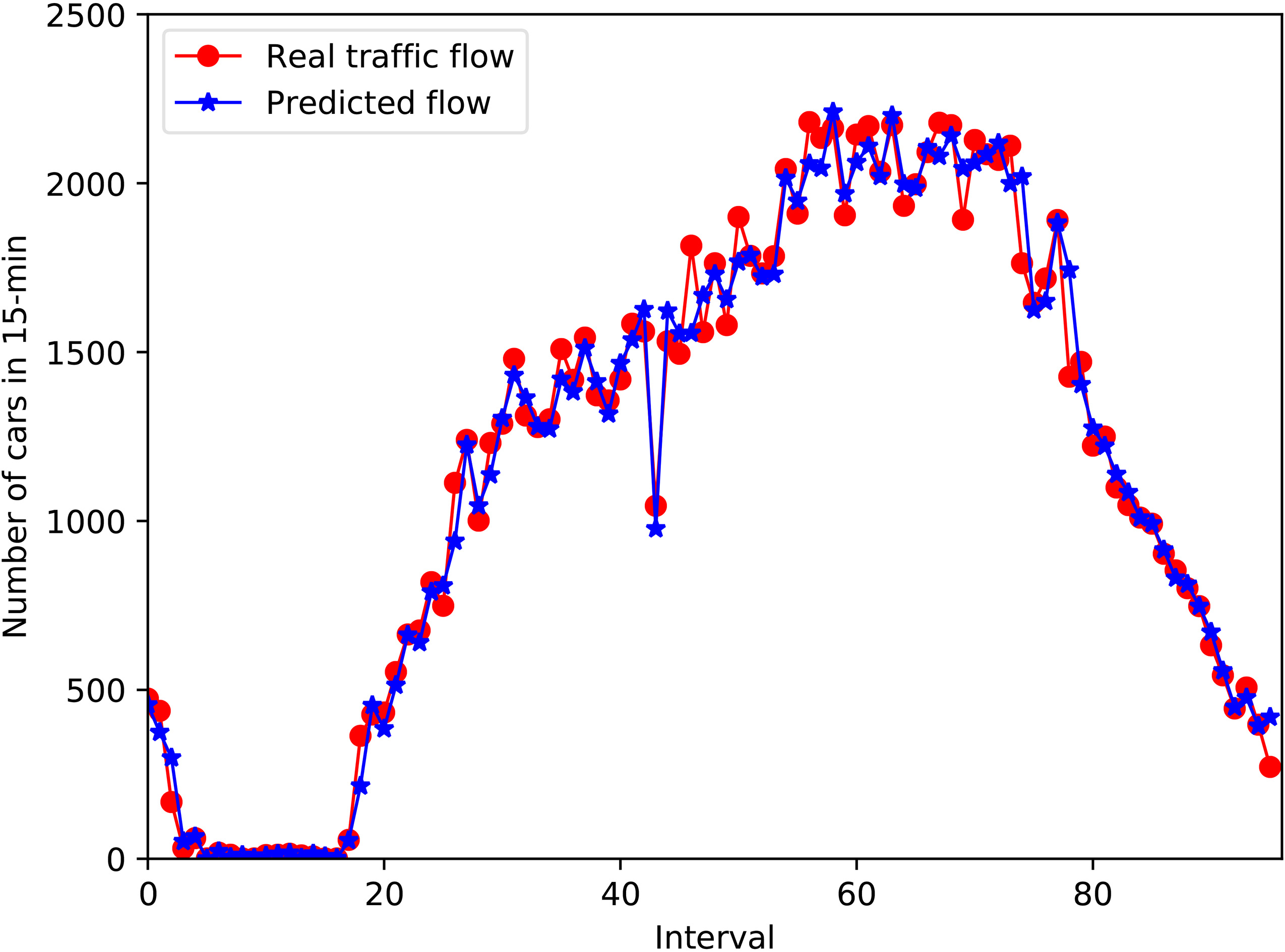

5.2 Validity of bayesian optimization for model parameter selection

Figure 5.

Comparing with SARIMA.

Figure 6.

Comparing with MLP-NN.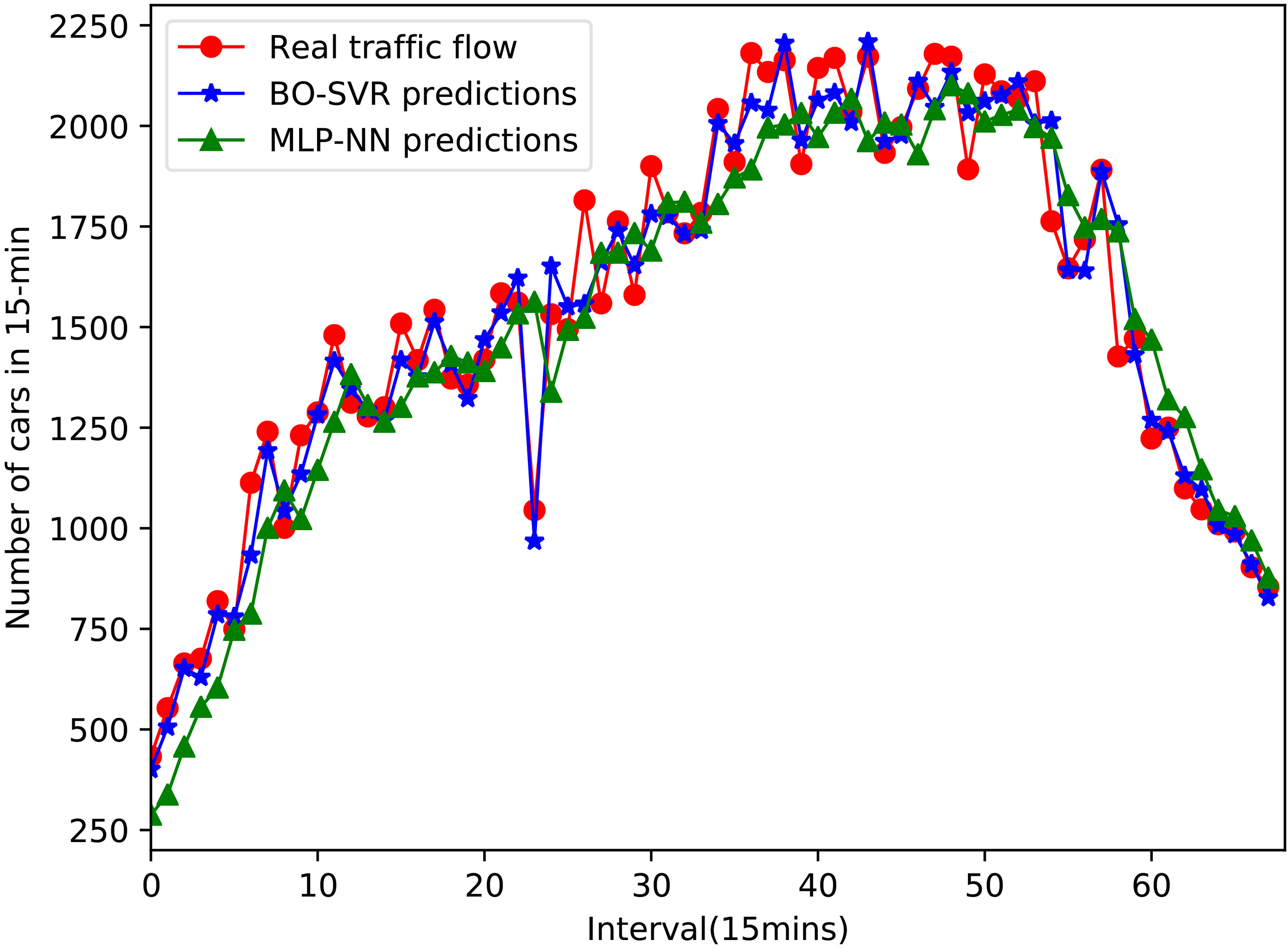

Figure 7.

Comparing with ERT.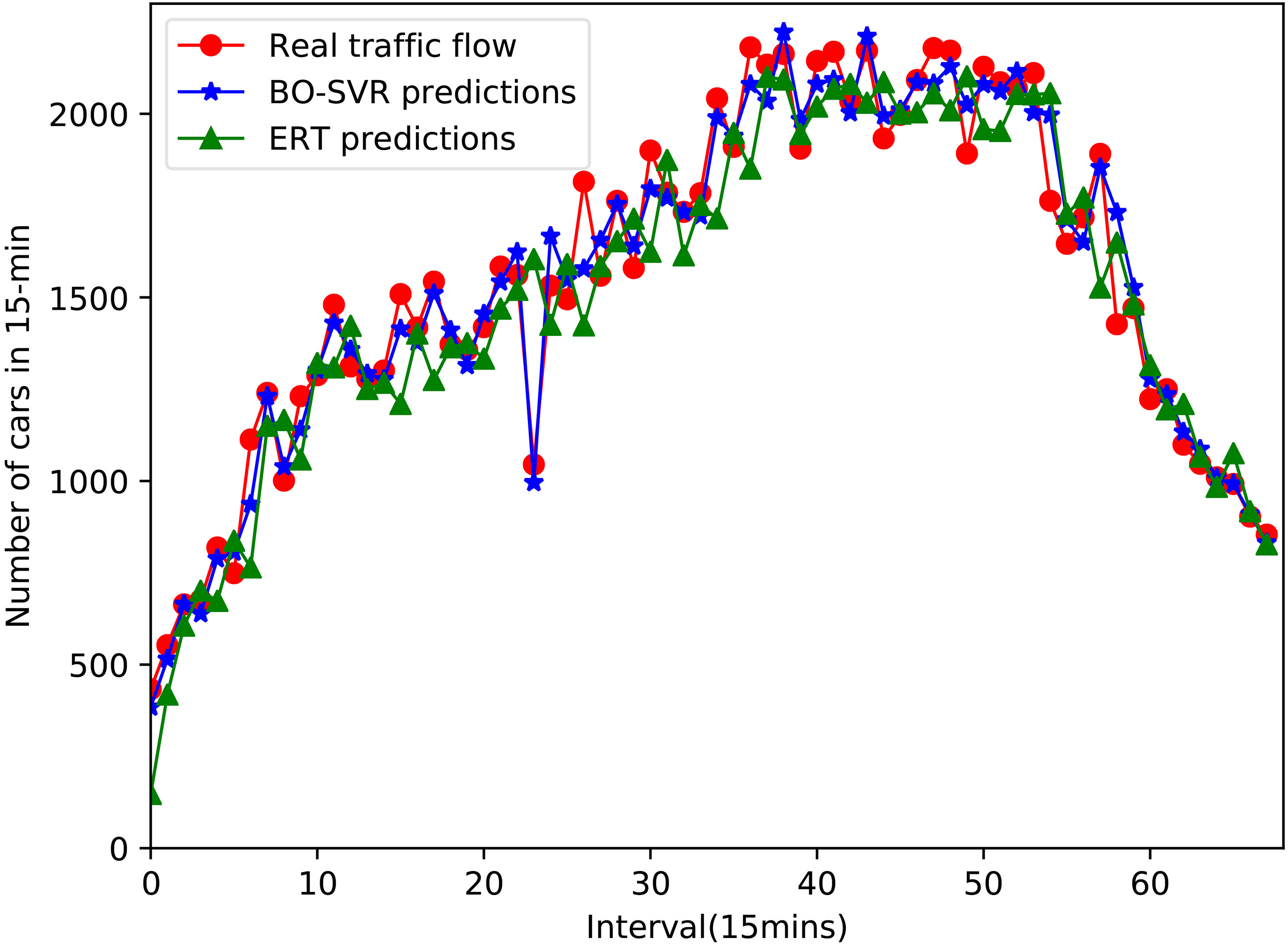

Figure 8.

Comparing with Adaboost.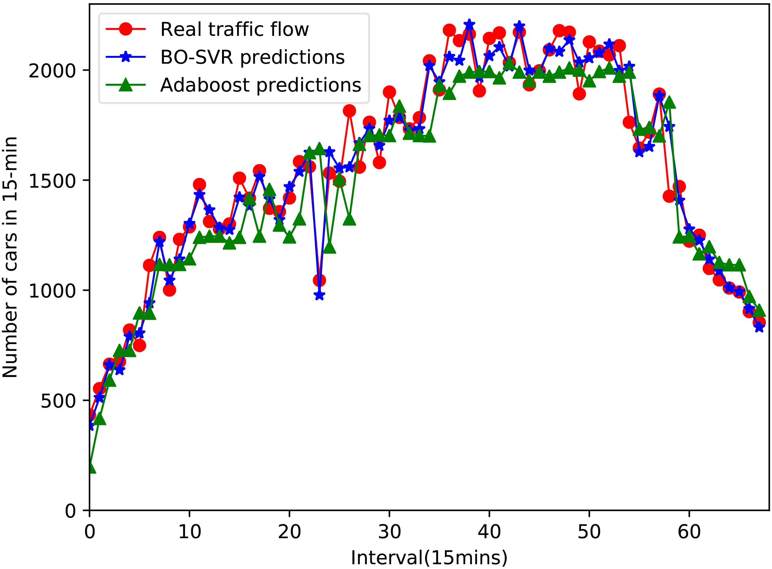

In this section, a contrast experiment is conducted to prove the validity of Bayesian Optimization used in choosing parameters of model. As mentioned above, there are three parameters needed to be optimized in the SVR model we proposed, which are $C$ , $\varepsilon$ and $\sigma$ . The experiment is as follows: There are four pairs of experiments. Using the Bayesian Optimization to choose parameters of SVR and choose zero parameter at first, namely, without Bayesian Optimization, and then increase one parameter each time. As to the parameters which are not optimized, the parameter of $C$ is set as 1 acquiescently. The $\varepsilon$ is set as 0.1 and the $\sigma$ is set as 1/n_features. These models are trained and tested using the same traffic flow data set and the data is collected from the detector in point 4. The time range selected is from 2017-9-25 to 2017-10-9. We use the data of the first 2 weeks as the training set and the remaining day as the testing set, the predicted interval is 15 minutes.

Table 1

Performance comparison of the MAPE for SARIMA, MLP-NN, ERT, Adaboost and our BO-SVR

	MAPE
	Detectors	SARIMA	MLP-NN	ERT	Adaboost	BO-SVR
Peak time 5:00 AM–10:00 PM	Point 1	91.25	89.58	110.42	179.43	83.33
(interval 5 mins)	Point 2	27.38	23.17	25.86	57.85	24.47
	Point 3	401.85	347.85	344.39	988.89	330.54
	Point 4	20.96	21.09	20.70	26.43	20.29
Peak time 5:00 AM–10:00 PM	Point 1	16.84	17.33	16.38	31.04	15.79
(interval 15 mins)	Point 2	19.70	16.33	14.40	46.02	15.52
	Point 3	647.45	117.75	100.39	981.63	59.56
	Point 4	6.89	6.29	5.92	9.87	6.21

Table 2

Performance comparison of the RMSE for SARIMA, MLP-NN, ERT, Adaboost and our BO-SVR

	RMSE
	Detectors	SARIMA	MLP-NN	ERT	Adaboost	BO-SVR
Peak time 5:00 AM–10:00 PM	Point 1	47.56	49.32	51.95	21.10	43.03
(interval 5 mins)	Point 2	71.29	74.53	80.48	108.74	73.67
	Point 3	70.41	68.07	68.06	92.48	66.16
	Point 4	46.32	49.84	46.66	53.52	47.54
Peak time 5:00 AM–10:00 PM	Point 1	72.87	104.78	134.85	163.68	101.23
(interval 15 mins)	Point 2	134.63	135.81	160.42	257.92	132.03
	Point 3	116.46	142.03	139.97	170.64	133.53
	Point 4	75.80	100.73	105.11	129.18	100.05

The prediction accuracy of these experiments is shown in Fig. 3. In Fig. 3, the abscissa represents the traffic flow forecasting model with different optimization parameters. The ordinate represents the prediction accuracy of each model. We can see the last column, which represents that the model of all parameters are optimized, is over 90% and outperforms all other models obviously. At the same time, we can also see that with the increase of optimization parameters, the accuracy of the model increases significantly. Therefore, it can be concluded that Bayesian optimization is effective for parameter selection of SVR-based short-term traffic flow prediction mode.

Table 3

Performance comparison of the MAE for SARIMA, MLP-NN, ERT, Adaboost and our BO-SVR

	MAE
	Detectors	SARIMA	MLP-NN	ERT	Adaboost	BO-SVR
Peak time 5:00 AM–10:00 PM	Point 1	31.59	36.58	37.50	38.37	30.95
(interval 5 mins)	Point 2	62.21	45.54	51.85	87.02	46.19
	Point 3	47.36	44.69	45.26	70.97	43.01
	Point 4	31.05	31.84	31.59	39.98	30.30
Peak time 5:00 AM–10:00 PM	Point 1	53.47	76.98	100.69	128.14	71.47
(interval 15 mins)	Point 2	111.86	103.23	111.17	213.98	100.13
	Point 3	96.94	104.66	97.15	139.85	96.43
	Point 4	60.00	71.81	71.52	102.72	71.63

Table 4

Performance comparison of 15 minutes traffic flow prediction at point 1 using three training sets at different time periods and different forecast methods

SARIMA			MLP-NN			ERT			Adaboost			BO-SVR
MAPE	RMSE	MAE	MAPE	RMSE	MAE	MAPE	RMSE	MAE	MAPE	RMSE	MAE	MAPE	RMSE	MAE
Training data set duration: 2017.9.25–2017.10.9
16.84	72.87	53.47	17.33	104.78	76.98	16.38	134.85	100.69	31.04	163.68	128.14	15.79	101.23	71.47
Training data set duration: 2017.6.25–2017.7.9
89.22	65.41	62.04	46.85	67.71	52.63	60.99	62.64	49.68	121.45	92.27	73.34	33.70	61.46	46.67
Training data set duration: 2016.9.25–2016.10.9
20.36	88.01	69.26	14.25	81.44	68.57	12.68	87.87	72.87	21.97	112.12	100.18	13.63	81.91	67.71

5.3 Comparison results

In this section, we mainly discuss the overall performance of the proposed BO-SVR method. We use the data collected from the four detectors to experiment separately. The time range is from 2017-9-25 to 2017-10-9. The training set and the data set are set as before. We first give an illustration of the 15 minutes prediction of traffic flow and that of real traffic flow in one day on node 3, it is shown in Fig. 4. We can see that there is peak time in one day’s traffic flow, which is from 5:00 AM to 10:00 PM. As the purpose of traffic flow prediction is to relieve traffic pressure during peak time. Thus, we mainly analyze the effects of the proposed forecast model at peak time.

For the purpose of evaluating the performances of the proposed method, we compare the proposed method with other methods. The comparing methods include the classical time series forecasting method SARIMA, the ensemble learning method ERT and Adaboost, and Multi-Layer Perceptron(MLP-NN). As for MLP-NN, hidden layer is set to five. The network training method is gradient descent with momentum adaptive learning back propagation algorithm, the learning rate is set to 0.3. For all experiments, same training set and test set are used. Figures 5–8 show the 15-minute flow forecast results of proposed algorithm compared with other algorithms at peak hours 5:00 AM to 10:00 PM on node 1.

From the line chart, we could see that the real traffic flow value has a lowest point at time index 24. There may be a traffic jam at this point. It is obviously that only the proposed BO-SVR and SARIMA have predicted this sudden drop. Other methods including MLP-NN, ERT and Adaboost are affected by this incident, so they deviate from the actual flow. SARIMA offsets a lot of real values at adjacent moments. Only the proposed method BO-AVR is capable of eliminating this influence best.

In terms of prediction accuracy, SARIMA forecasts are very unstable during peak periods. This is because that the SARIMA model parameters are fixed. The predicted value of MLP-NN has a significant backward relative to the true value. This may be the reason that inappropriate parameters have been chosen so that the model is not well informed of trends in the traffic flow time series. ERT apparently has a trend below the true value at the peak stage. Adaboost is also the case, and the effect is more unstable. The predictions of BO-SVR are the best, and it can see that the model has learned the inherent tendency of traffic flow time series changes.

The Table 1 to Table 3 show the MAPE, RMSE value and MAE value calculated by different prediction methods at four detectors after running 5 times. The forecast range is the peak time of October 9, 2017. The forecast period is divided into 5 minutes and 15 minutes. From the previous introduction of the evaluation metrics, we know that MAPE is the representative of the relative error of the predicted values, RMSE and MAE represent the absolute error. Since the test data set contained midnight time period, the number of vehicles at this time is almost zero. Therefore, the overall relative error MAPE becomes large, especially at points 1 and 3. Similarly, compared to the 15-minute traffic flow time series, the 5-minute traffic flow is smaller. So, the relative error in 5-minute prediction is greater, while the absolute error is smaller for the RMSE and MAE. Therefore, it can be concluded from the longitudinal comparison of the tables that our experimental results are logical and representative.

By comparing MAPEs horizontally, we find that our BO-SVR predictions are better than the other methods except for individual rows. Especially at point 3, the effect of improvement is obvious. This shows that BO-SVR is more suitable for prediction of non-stationary sequence. In Tables 2 and 3, BO-SVR is also significantly better than other algorithms, and the actual error can be reduced by about 3% to 5% than other optimal algorithms. By analyzing the predicted results from different perspectives, it could be concluded that the proposed BO-SVR method is effective for short-term traffic flow prediction.

In order to better verify the effectiveness of the algorithm and explore the traffic flow characteristics in different years and different seasons. We select three different phases of data sets for repeated experiments from 2016-9-25 to 2016-10-9, from 2017-6-25 to 2016-7-9 and from 2017-9-25 to 2017-10-9 respectively. The Table 4 shows the comparison results of 15 minutes of traffic flow prediction at the point 1 using three training sets at different time periods and different forecast methods. The experimental results show that the proposed BO-SVR method can still achieve good results and has good generalization ability in different data sets. At the same time, we can also draw conclusions from the experimental data. Comparing with the quarter, traffic flow data among different years is more relevant, because of the fluctuations between different seasons. Therefore, when conducting long-term traffic flow forecasting research under big data in the future, we can consider using the previous years’ data to increase the accuracy of the forecast.

6. Conclusion

In this paper, we propose a regression method based on Support Vector Machine and Bayesian Optimization, called BO-SVR, to predict short-term traffic flow. Using the idea of SARIMA to eliminate the non-stationary of traffic flow data and using Bayesian optimization to select parameters of support vector regression. By compared with classical SARIMA, MLP-NN, ERT and Adaboost methods in typical sections of real road. The results show the superior advantage and generalization of BO-SVR in different conditions. For future work, we may consider to use larger traffic flow data to construct a deep architecture of traffic flow forecasting and to acquire more accurate prediction results. Furthermore, we will focus on some problems in reality, such as missing data and data noise, which have influence on prediction performance, so that we can build a robust prediction system.

Footnotes

Acknowledgments

This work was partially supported by the National Natural Science Foundation of China (grants nos. 61301148, 61272061, 61502162 and 61702175), the Fundamental Research Funds for the Central Universities of China, Fund of State Key Laboratory of Geoinformation Engineering (no. SKLGIE2016-M-4-2), Hunan Natural Science Foundation of China (no. 2018JJ2059), and Open Fund of State Key Laboratory of Integrated Services Networks (no. ISN17-14).

Appendix

Due to the characteristics of the traffic flow data, there is seasonality in weekly data and daily data. Seasonality usually causes the series to be non-stationary, therefore, we perform seasonal differential processing on the data to eliminate seasonality and non-stationarity. Then, By combining the data from the previous moment, the previous day, and the previous week, the following data set are constructed:

$\{{\left({X,y}\right)|X\!={{\left[{{v_{i-1,}}{v_{i-1}}-{v_{i-2}},{v_{i-\textit% {week}}},{v_{i-\textit{week}}}-{v_{i-week-1}},{v_{i-\textit{day}}},{v_{i-% \textit{day}}}-{v_{i-\textit{day}-1}}}\right]}^{T}},y={v_{i}}}\}$

Then, due to the different dimensions between the different attributes, this will affect the results of the experiment. In order to eliminate the dimensional impact between the attributes, the previously constructed data set is normalized such that the individual indicators are at the same order of magnitude.

References

Box

G.E.P.

and Jenkins

G.M.

, Time Series Analysis Forecating and Control, HOlden-Day, 1970.

Brochu

Cora

V.M.

and Freitas

N.D.

, A tutorial on bayesian optimization of expensive cost functions, with application to active user modeling and hierarchical reinforcement learning, Computer Science, 2010.

Drucker

Burges

C.J.C.

Kaufman

Smola

A.J.

and Vapnik

, Support vector regression machines, Advances in Neural Information Processing Systems 28(7) (1996), 779–784.

Guo

Bai

and Ma

, Time series prediction method based on ls-svr with modified gaussian rbf, In International Conference on Neural Information Processing, 2012, pages 9–17.

Jones

D.R.

, A taxonomy of global optimization methods based on response surfaces, Journal of Global Optimization 21(4) (2001), 345–383.

Joy

T.T.

Rana

Gupta

and Venkatesh

, Hyperparameter tuning for big data using bayesian optimisation, In International Conference on Pattern Recognition, 2017, pages 2574–2579.

Kushner

H.J.

, A new method of locating the maximum point of an arbitrary multipeak curve in the presence of noise, Journal of Fluids Engineering 86(1) (1964).

Lin

Zhang

Qiao

Liu

and Yu

, A parameter choosing method of svr for time series prediction, In Young Computer Scientists, 2008. Icycs 2008. the International Conference for, 2008, pages 130–135.

Lippi

Bertini

and Frasconi

, Short-term traffic flow forecasting: An experimental comparison of time-series analysis and supervised learning, IEEE Transactions on Intelligent Transportation Systems 14(2) (2013), 871–882.

10.

Duan

Kang

and Wang

F.Y.

, Traffic flow prediction with big data: A deep learning approach, IEEE Transactions on Intelligent Transportation Systems 16(2) (2015), 865–873.

11.

and Ying

, Research of traffic flow forecasting based on neural network, In International Symposium on Intelligent Information Technology Application, 2009, pages 104–108.

12.

Mockus

Tiesis

and Zilinskas

, The application of Bayesian methods for seeking the extremum, 1978.

13.

Okutani

and Stephanedes

Y.J.

, Dynamic prediction of traffic volume through kalman filtering theory, Transportation Research Part B 18(1) (1984), 1–11.

14.

Rasmussen

C.K.W.C.E.

, Gaussian Processes for Machine Learning, MIT Press, 2006.

15.

Shi

and Eberhart

R.C.

, Empirical study of particle swarm optimization, 2002.

16.

Snoek

Larochelle

and Adams

R.P.

, Practical bayesian optimization of machine learning algorithms, In International Conference on Neural Information Processing Systems, 2012, pages 2951–2959.

17.

Zhang

and Yu

, Short-term traffic flow prediction based on incremental support, vector regression. In International Conference on Natural Computation, 2007, pages 640–645.

18.

Sun

Zhang

and Yu

, A bayesian network approach to traffic flow forecasting, IEEE Transactions on Intelligent Transportation Systems 7(1) (2006), 124–132.

19.

Teh

Y.W.

Seeger

and Jordan

, Semiparametric latent factor models, Artificial Intelligence and Statistics, 2005, pages 565–568.

20.

Voort

M.V.D.

Dougherty

and Watson

, Combining kohonen maps with arima time series models to forecast traffic flow, Transportation Research Part C Emerging Technologies 4(5) (1996), 307–318.

21.

Xie

Zhang

and Ye

, Short-term traffic volume forecasting using kalman filter with discrete wavelet decomposition, Computer-aided Civil and Infrastructure Engineering 22(5) (2007), 326–334.

22.

Kong

Q.J.

and Liu

, Short-term traffic volume prediction using classification and regression trees, IEEE Intelligent Vehicles Symposium (IV) 36(1) (2013), 493–498.

23.

Zhang

and Zhuang

, Short-term traffic flow forecasting based on markov chain model, In Intelligent Vehicles Symposium, 2003. Proceedings. IEEE, 2003, pages 208–212.