Hybrid data stream clustering by controlling decision error

Abstract

Data stream clustering is an unsupervised learning method for sequential data. Data stream clustering has some challenging issues, such as handling limited memory, dealing with evolving clusters, and detecting noise data. We propose a hybrid data stream clustering method that combines model-based clustering and density-based clustering. The proposed method finds evolving clusters quickly and obtains cluster information easily. We use multiple hypothesis testing to handle noise data by controlling a decision error. In this testing method, we employ the positive false discovery rate as the decision error. We use a density-based algorithm to discover cluster evolution from newly arrived data. Then, we estimate a Gaussian mixture model and update the clustering results by combining past cluster information and the cluster information for newly arrived data. We applied the proposed method to several synthetic and real datasets. The experimental results demonstrate that the proposed method works effectively for a data stream that includes noise data. In addition, the proposed method yields robust results relative to input parameters compared to an existing density-based data stream clustering method.

Keywords

False discovery rate Gaussian mixture multiple testing noise data

1. Introduction

As technology advances, a huge amount of data is generated in many fields. Interest in data stream mining, which extracts meaningful information from data streams, also has increased. For example, data stream mining can be applied to monitoring network traffic, where data can change relative to user status, location, or connection purpose. The volume and speed of data streams, i.e., sequences of continuous data generated from networked devices and sensors, are increasing rapidly [19].

Data stream mining differs from conventional data mining, which uses a finite data set and can recall data as required. In contrast, data stream mining uses an infinite sequential data stream that cannot be recalled. Moreover, typically data streams are large and used data should be discarded due to limited storage and memory capacity. Data clustering finds meaningful information by grouping similar multi-dimensional data points. Data stream clustering is an unsupervised learning method for sequential data streams. According to Amini et al. [2], data stream clustering methods can be classified into five categories: partitioning, hierarchical, grid-based, density-based, and model-based methods. Each of them will be described and related algorithms will be surveyed in Section 2.1.

Responding quickly to cluster evolution is a significant issue in data stream clustering. Many density-based clustering algorithms have been developed to address this issue. However, it is typically difficult for density-based clustering to summarize cluster information and find optimal parameters for the best results. Therefore, we develop a hybrid algorithm for data stream clustering that combines model-based and density-based clustering methods to handle cluster evolution quickly and find optimal parameters efficiently. Further, existing data stream clustering algorithms have not dealt with clustering errors particularly when they are associated with noise data. In this paper, noise data indicates an insignificant data point (object) which does not belong to any cluster. The proposed algorithm can control the clustering decision error using multiple tests when handling noise data. A decision error occurs if a true cluster member is declared as noise and vice versa. The positive false discovery rate (pFDR) is adopted to control the error rate. The pFDR is defined as the expected proportion of false positives among all rejected hypotheses given that the number of rejected hypotheses is greater than zero [25].

The remainder of this paper is organized as follows. Section 2 reviews data stream clustering methods and introduces Density-Based Spatial Clustering of Applications with Noise (DBSCAN) [11], a well-known density-based clustering method, and DenStream [5], a popular data stream clustering method based on DBSCAN. Section 3 presents the proposed clustering method. We describe experiments with synthetic and real datasets to evaluate the proposed method in Section 4. Finally, Section 5 concludes the paper by summarizing the results.

2. Related works

2.1 Existing data stream clustering methods

Data stream clustering methods can be classified into five categories: partitioning, hierarchical, grid-based, density-based, and model-based methods [2]. In this section, we briefly explain about each category and introduce some related algorithms.

A partitioning clustering algorithm divides all data points (or objects) into $K$ groups ( $K$ is usually pre-defined), and clusters are constructed by optimizing clustering criterion. Generally, partitioning clustering algorithm makes $K$ -initial clusters randomly or by some heuristics and then iteratively reassign objects according to updated information of clusters. For example, CluStream [1] is a data stream clustering method based on k-means clustering. It follows the online-offline learning procedure, where online phase handles new data and offline phase updates clusters.

A hierarchical clustering algorithm is composed of agglomerative (bottom-up) and divisive (top-down) methods. The agglomerative method sets each data as a cluster and merges them sequentially and the divisive method assigns all data into one cluster and divides the cluster into smaller ones. These algorithms repeatedly updates until pre-defined stopping criteria are satisfied. ClusTree [17] generates micro-clusters and merges them based on a hierarchical index.

Grid- and density-based clustering methods assume that the density of a cluster area is high and the density of a noise area is low [26]. A grid-based clustering algorithm divides data space into grid structure. In each grid, the number and information of data points are stored to determine if it is dense area or sparse area, which corresponds to clustered data points and noise data points, respectively. MR-Stream makes use of STING [28], which is grid-based method, and constructs a tree of grid cells. MR-Stream merges child nodes of the same parent node if all of them are dense or sparse to save memory and cluster fast. More recently, Hua et al. [14] developed an algorithm combining the advantages of grid- and density-based methods by using the local density of each object and the distance from the objects.

A density-based clustering method finds a dense area and increases its size continuously by adding dense neighborhoods. DenStream [5] is a density-based clustering algorithm for data streams. Representative density-based clustering algorithms, DBSCAN and DenStream, will be discussed in more detail in Section 2.2. Recently, Chen and He [6] proposed a new density-based algorithm so as to cluster mixed data stream accurately. Ding et al. [10] presented an adaptive density-based algorithm for mixed type data.

Model-based clustering assumes that data points are generated by an underlying distribution, which is usually estimated by the expectation-maximization (EM) method [9] and clustering is performed based on the estimated distribution. Model-based methods can handle noise data by estimating the responsibility of each data point, where a data point with lower responsibility is declared as noise. In a model-based method, the data stream is typically assumed to follow a Gaussian mixture distribution. Dang et al. [7] proposed a data stream clustering method using a time-based sliding window model with a set of micro-clusters following a multivariate normal distribution. Song and Wang [24] estimated a Gaussian mixture distribution for new data at each time window. Then, they tested for mean and covariance equivalence for new and existing components. Two components are merged if they pass this test; otherwise, a new component will be a separate cluster.

Until recently, many data stream clustering algorithms have been proposed. However, each algorithm has its own advantage and limitation. A recent review article by Nguyen et al. [20] on data stream mining summarizes pros and cons of each data stream clustering category. Partitioning-based clustering is simple and relatively efficient. However, a user needs to pre-define the number of clusters, which has an impact on clustering results. It is limited to only spherical clusters. Hierarchical clustering can find meaningful structure of clusters, but searching the structure is too complex and sensitive to the order of the data. Grid- and density-based clustering can find arbitrary-shape clusters and is robust to noise points. Grid-based clustering is generally fast, but may not be proper in high-dimensional data because the result is dependent on the grid granularity. Density-based clustering requires many parameters such as density or noise thresholds to find arbitrary-shape clusters. In addition, it is difficult to detect clusters with different densities. Finally, model-based clustering is simple and can make use of domain knowledge but it highly depends on model assumptions.

More recent data stream clustering algorithms combine two or more approaches to overcome their limitations. For example, ADStream [10] takes advantages of density-based clustering and affinity propagation clustering to handle irregular data streams such as noise or outliers. The affinity propagation is similar with partitioning methods, which do not require pre-defined number of clusters. DEGDS [14] combines the advantages of grid- and density-based clustering algorithm. DEGDS uses a local density and distance matrix to get clustering centers in the grid and then extends the result or merges grid boundaries by using density concepts. This removes unsuitable selection of initial centroid and saves the memory. Besides, Str-FSFDP [6] develops a density-based clustering algorithm, which uses a novel distance metric in order to handle mixed type data.

2.2 DBSCAN and DenStream

In this paper, the performance of the proposed method is compared to that of DenStream [5]. Thus, here, we describe DenStream in detail. First, we explain DBSCAN, a well-known density-based clustering method, because DenStream is based on DBSCAN.

Density-based clustering assumes that a cluster area is dense and other areas are spare. The most popular density-based clustering algorithm is DBSCAN [11]. The input DBSCAN parameters are the minimum number of points (MinPts) and $\epsilon$ . They define the neighborhood of a point to be points that are distributed within $\epsilon$ . If the number of the neighbors of a point is greater than MinPts, the point will be a core point. If $q$ is a core point and $p$ is included in the neighborhood of $q$ , then $p$ is directly density-reachable from $q$ . To extend this concept, $p$ is density-reachable from $q$ if there is a chain of points $p_{{1}}=q,p_{{2}},\dots p_{n}=p$ such that $p_{i+1}$ is directly density-reachable from $p_{i}$ . Point $p$ is density-connected from $q$ if there is a point $o$ such that both $p$ and $q$ are density-reachable from $o$ . A cluster is defined as a set of density-connected data points. Noise points are not included in any clusters. DBSCAN finds clusters and noise simultaneously, and there is no limitation relative to cluster shape or size. A clustering result is highly sensitive to the MinPts and $\epsilon$ values; however, some authors have suggested optimal values [8, 11].

DenStream assumes a damped window model, in which the weight of each data point decreases exponentially over time with a fading function. The micro-cluster (MC) corresponds to $\epsilon$ -neighborhood in DBSCAN. Cao et al. [5] defined a core MC similarly to the core point of DBSCAN, i.e., a potential core MC (p-MC) and an outlier MC (o-MC). The p-MCs and o-MCs can be maintained incrementally. If no points are merged into a MC in a given time interval, then the weight will decrease. DenStream can be divided into two parts: an online part for MC maintenance and an offline part to generate the final clusters. The online part proceeds each time new data arrives. When a new data point arrives and finds the nearest MC, we create a new o-MC. The offline part proceeds at a given time interval or at the user’s request.

The DenStream algorithm involves several parameters, including $\epsilon$ , $\mu$ , $\beta$ , and $\lambda$ . In this study, we fix parameters $\beta$ and $\lambda$ to 0.2 and 0.001, respectively, while we consider several values for $\epsilon$ and $\mu$ .

3. Proposed hybrid data stream clustering method

We propose a data stream clustering method that combines model-based and density-based clustering. It is assumed that a new dataset arrives at each time window and that a new dataset consists of clustered data plus noise. We assume that the clustered data follow a Gaussian mixture with an unknown number of components and noise data are spread randomly. The characteristics of a new dataset may change over consecutive time windows.

Assume that a d-dimensional data point $\bm{x}$ follows a Gaussian mixture with K unknown components whose probability density function is given as follows:

$\displaystyle f(\bm{x}|\Theta_{K})=\sum_{k=1}^{K}\alpha_{k}n_{k}(\bm{x}|\bm{% \mu}_{k},\bm{\Sigma}_{k})$ (1)

where ${\alpha}_{k}$ is the mixing weight of the $k$ -th component and $n_{k}(\bm{x}|\bm{\mu}_{k},\bm{\Sigma}_{k})$ is the d-dimensional multivariate normal density having mean vector $\bm{\mu}_{k}$ and covariance matrix $\bm{\Sigma}_{k}$ . Here $\Theta_{K}=\{{\alpha}_{k},\bm{\mu}_{k},\bm{\Sigma}_{k},k=1,\dots,K\}$ represents unknown model parameters.

3.1 Outline of the proposed algorithm

The proposed algorithm consists of two phases, i.e., initial and incremental phases. The initial phase is used only at the first time window and the incremental phase applies to subsequent time windows. We estimate the Gaussian mixture distribution and perform multiple hypothesis testing in the initial phase. Whenever a new dataset arrives, we check cluster evolution and update the cluster result in the incremental phase. The required steps in our two-phase procedure are as follows.

Initial phase

(1)
Eliminate noise points using DBSCAN. This step helps estimate the Gaussian mixture distribution more accurately.
(2)
Estimate the Gaussian mixture distribution using incremental EM. We must find an optimal number of components in the Gaussian mixture.
(3)
Apply multiple hypothesis testing and classify data as cluster members or noise points.

Incremental phase

(1)
Assign data points from a new dataset to existing clusters based on the previous information.
(2)
Find new clusters.
(3)
Make a merge or split decision for the clusters.
(4)
Find clusters to remove.
(5)
Update the cluster result.

3.2 Estimating Gaussian mixture using Incremental EM

An EM method may be sensitive to noise points or outliers. Thus, we separate these noise points from the data using DBSCAN before estimating a Gaussian mixture using an EM algorithm. Essentially, data points that are not grouped minimally will be declared noise points. Other points will be declared non-noise points. As a result, we obtain a Noise_data set and a Non_noise_data set. These two sets are divided to estimate a more accurate Gaussian mixture distribution. These two sets are updated after clustering.

We use the Non_noise_data set to estimate Gaussian mixture distribution with an unknown number of cluster components. Ueda et al. [27] and Blekas and Lagaris [4] proposed Incremental EM methods to estimate a mixture model with an unknown number of components. We use the method proposed by Blekas and Lagaris [4], which starts with two components and applies the split step and the merge step until the best mixture model is obtained. Here, we use the Bayesian information criterion (BIC) [23] for the model selection, while Blekas and Lagaris [4] originally used the log-likelihood. The BIC is given as follows:

$\displaystyle\text{BIC}=-2\times\ln L+p\times\ln(N)$ (2)

where ln $L$ is the log-likelihood of the given model, $p$ is the number of free parameters to be estimated, and $N$ is the number of data points. $p=(K-1)+K*d+K*(d+1)*d/2$ for the Gaussian mixture when all covariance matrices differ and has a full model. A model with a smaller BIC value is considered a better model.

3.3 Multiple hypothesis testing for the proposed method

We divide data into noise points and cluster members using a multiple hypothesis testing. Lee and Jun [18] and Park et al. [21] proposed clustering methods using multiple hypothesis testing. The key idea in those papers is that a clustering problem is viewed as multiple hypothesis testing to control decision error. Here, we apply a similar idea to a data stream. However, we only use $N$ hypotheses simultaneously, while those previous studies dealt with $N$ hypotheses $K$ times, where $N$ is the number of data points and $K$ is the number of mixture components.

Let ${\bm{x}}_{i}$ , where $i=1,\ldots,N$ , be the $i$ -th data point. We consider the multiple hypothesis testing of $H_{1},H_{2},\dots,H_{N}$ , where the null and alternative hypotheses in $H_{i}$ are as follows.

Null hypothesis: ${\bm{x}}_{i}$ comes from the Gaussian mixture.

Alternative hypothesis: ${\bm{x}}_{i}$ does not comes from the Gaussian mixture.

If the null hypothesis is true, then the $p$ -value of ${\bm{x}}_{i}$ is calculated as follows.

$\displaystyle p_{i}=\int_{\{\bm{y}|\bm{f}(\bm{y})<f({\bm{x}}_{i})\}}f(\bm{y}|% \Theta_{K})d\bm{y}$ (3)

If $K$ is greater than 1, we cannot obtain the closed form solution of the $p$ -value. Thus, we propose the following approximation method to calculate the $p$ -value:

$\displaystyle p_{i}=\int_{\{\bm{y}|\bm{f}(\bm{y})<f({\bm{x}}_{i})\}}\sum^{K}_{% k=1}{\alpha}_{k}n_{k}(\bm{y}|\bm{\mu}_{k},\bm{\Sigma}_{k})d\bm{y}\approx\sum^{% K}_{k=1}{\alpha}_{k}\int_{\{\bm{y}|n_{\bm{k}}(\bm{y}|{\bm{\mu}}_{k},{\bm{% \Sigma}}_{k})<{\nu}_{ik}\}}n_{k}(\bm{y}|\bm{\mu}_{k},\bm{\Sigma}_{k})d\bm{y}$ (4)

where

$\displaystyle{\nu}_{ik}=\min\left\{\frac{n_{k}(\bm{x}_{i}|\mu_{k},\bm{\Sigma}_% {k})}{\alpha_{k}},n_{k}(\bm{\mu}_{k}|\bm{\mu}_{k},\bm{\Sigma}_{k})\right\}.$

Although the result was not reported here, the above approximation provides quite accurate $p$ -values for a smaller number of components.

Using the set of calculated $p$ -values $\{p_{1},\dots,p_{N}\}$ , we obtain the pFDR as follows [25]:

$\displaystyle\text{pFDR}(\bm{x}_{i},\lambda)=\frac{\#\{p_{j}>\lambda\}p_{i}}{(% 1-\lambda)\max[1,\#\left\{p_{j}<p_{i}\right\}]}$ (5)

where $\#\{\textit{argument}\}$ is the number of data points satisfying the “argument”. Here, $\lambda$ can be chosen arbitrarily between 0 and 1, but a small value, such as 0.15, is recommended by Park et al. [21].

Then, we classify each data point as noise or a cluster member based on the pFDR. Let $q^{*}$ be the target pFDR level. If $\text{pFDR}({\bm{x}}_{i},\lambda)<q^{*}$ , data point ${\bm{x}}_{i}$ is declared as noise. Otherwise, the data point ${\bm{x}}_{i}$ is declared a cluster member. Furthermore, we can assign ${\bm{x}}_{i}$ to a cluster by computing the membership weight from the EM algorithm. The membership weight of ${\bm{x}}_{i}$ to the $k$ -th cluster is obtained as follows.

$\displaystyle w_{ik}=\frac{n_{k}(\bm{x}_{i}|\bm{\mu}_{k},\bm{\Sigma}_{k})% \alpha_{k}}{\sum^{K}_{m=1}{n_{m}(\bm{x}_{i}|\bm{\mu}_{m},\bm{\Sigma}_{m})% \alpha_{m}}}$ (6)

Here, let $c=\text{arg}\text{max}_{k}w_{ik}$ . Then, we assign $\bm{x}_{i}$ to the $c$ -th cluster if $\text{pFDR}(\bm{x}_{i},\lambda)\geqslant q^{*}$ .

3.4 Incremental phase

The incremental phase is applied from the second time window and thereafter. We define the following notations.

$N^{t}$ : number of data points to arrive at the $t$ -th time window $K^{t}$ : number of clusters at the $t$ -th time window $N^{t}_{k}$ : number of points among $N^{t}$ assigned to the $k$ -th cluster ${\bm{m}}^{t}_{k}$ : sample mean vector of the $k$ -th cluster from $N^{t}_{k}$ data points ${\bm{S}}^{t}_{k}$ : sample covariance matrix of the $k$ -th cluster from $N^{t}_{k}$ data points $\rho$ : fade rate $n^{t}_{k}$ : updated number of points of the $k$ -th cluster at the $t$ -th time window $\bm{\hat{\mu}}^{t}_{k}$ : updated mean vector estimate of the $k$ -th cluster at the $t$ -th time window $\bm{\hat{\Sigma}}^{t}_{k}$ : updated covariance matrix estimate of the $k$ -th cluster at the $t$ -th time window

3.4.1 Assigning new data points to a cluster using previous cluster information

Initially, we assign new data points at the $t$ -th time window to one of the clusters using the cluster information at the ( $t-1$ )-th time window. We first need to calculate the $p$ -values for each component of the Gaussian mixture. Here, let $p_{ik}$ ( $i=1,\ldots,N^{t}$ ) be the p-values of the $k$ -th component ( $k=1,\ldots,K^{t-1}$ ). Then, we obtain the proportion of cluster members belonging to the $k$ -th component as follows.

$\displaystyle\omega_{k}(\lambda)=\min\left\{1,\frac{\#\{p_{ik}>\lambda)}{\left% (1-\lambda\right)N^{t}}\right\},k=1,\ldots,K^{t-1}$ (7)

We consider that the $k$ -th cluster has $\omega_{k}(\lambda)*N^{t}$ members. We sort the $p$ -values in descending order and select the first $\omega_{k}(\lambda)*N^{t}$ (or a rounded value if needed) data points as the $k$ -th cluster members. If there exist data points that have been assigned to more than two clusters, we select one cluster randomly. The unassigned data points are temporarily classified as noise points.

3.4.2 Finding new clusters

We find new clusters, if any exist, as follows.

1.
Apply DBSCAN to temporary noise points to form clusters. Here, let $D^{\textit{new}}_{i},i=1,\dots,K^{\textit{new}}$ be the DBSCAN cluster result.
2.
If $\left|D^{\textit{new}}_{i}\right|>$ min_cluster_num, then $D^{\textit{new}}_{i}$ can potentially be a new cluster. However, this may be a part of the existing clusters. Find the closest existing cluster, e.g., C ${}_{\text{c}}$ to $D^{\textit{new}}_{i}$ , where $\left|D^{\textit{new}}_{i}\right|>$ min_cluster_num in terms of Mahalanobis distance. Then, after combining the members in C ${}_{\text{c}}$ and $D^{\textit{new}}_{i}$ , we estimate two Gaussian mixture models having one and two components, respectively. If the BIC of the Gaussian mixture model with two components is smaller than the model with one component, then $D^{\textit{new}}_{i}$ will be declared a new cluster. Otherwise, members in $D^{\textit{new}}_{i}$ are assigned to an existing cluster according to the responsibilities based on the previous cluster information. If $\left|D^{\textit{new}}_{i}\leqslant\right|\text{min\_cluster\_num}$ , those data points are considered as noise points.

3.4.3 Merge/split decision

Existing clusters with newly added members may be merged or split. We make this decision using the SMILE algorithm [4]. First, we repeat the SMILE algorithm merge operation on the set of existing clusters with newly added members until the BIC does not decrease further. Then, we repeat the SMILE algorithm split operation until the BIC does not decrease.

3.4.4 Finding clusters to remove

We remove clusters whose number of members is less than a specified number. The members in the removed cluster, if any, will be allocated to the closest cluster.

3.4.5 Updating the cluster result

Through the above steps, we identify all clusters for the t-th time window. We update the number of points, as well as the mean and covariance matrix of each cluster as follows.

$\displaystyle n^{t}_{k}=\rho n^{t-1}_{k}+N^{t}_{k}$ (8) $\displaystyle\bm{\hat{\mu}}^{t}_{k}=\frac{\rho n^{t-1}_{k}\bm{\hat{\mu}}^{t-1}% _{k}+N^{t}_{k}\bm{m}^{t}_{k}}{n^{t}_{k}}$ (9) $\displaystyle\bm{\hat{\Sigma}}^{t}_{k}=\frac{\rho n^{t-1}_{k}\bm{\hat{\Sigma}}% ^{t-1}_{k}+N^{t}_{k}{\bm{S}}^{t}_{k}}{n^{t}_{k}}+\frac{\rho n^{t-1}_{k}\bm{% \hat{\mu}}^{t-1}_{k}(\bm{\hat{\mu}}^{t-1}_{k})^{T}+N^{t}_{k}{\bm{m}}^{t}_{k}(% \bm{m}^{t}_{k})^{T}}{n^{t}_{k}}-\bm{\hat{\mu}}^{t}_{k}(\bm{\hat{\mu}}_{k}^{t})% ^{T}$ (10)

We then perform multiple hypothesis testing (Section 3.3) to divide noise points (or not) and assign a non-noise point to a cluster index.

4. Experiments

We conducted experiments to evaluate the proposed method with synthetic and real datasets.

4.1 Validation measures

There are two types of validation measures for a cluster result, i.e., external criteria and internal criteria [13]. Internal criteria are validation measures that evaluate a cluster result using only inherent features in the dataset. The sum of square error and Silhouette [16] are typical internal criteria. External criteria use extrinsic information to evaluate cluster results. Popular external measures are purity, the Rand index [22] and the adjusted Rand index [15]. For a synthetic dataset to be generated from known clusters, external measures may be more objective.

In this study, we use the adjusted Rand index and mean purity for validation measures. We propose a method that can control the decision error by pFDR. If we know the true groups, then the actual pFDR can be obtained by the proportion of false decisions among all rejected hypotheses. Therefore, we report the actual pFDR for synthetic datasets to observe how well the proposed method controls the decision error.

4.2 Synthetic datasets

4.2.1 Two-dimensional synthetic data with evolving scenario

This synthetic dataset is generated from bivariate normal distributions over eight time windows with an evolving scenario. Figure 1 shows the dataset over time windows when noise points comprise 5% of the dataset. There are three clusters (blue, green, and cyan points) at the first and second time windows. A new cluster (magenta points) appears at the third time window. Two clusters (blue and magenta points) are merged at the fourth time window. A new cluster (yellow points) again appears at the fifth time window. The cluster with blue points at the fifth cluster is split into two clusters (blue and magenta points) at the sixth time window. The cluster with green points at the sixth time window disappears at the seventh time window. Finally, the cluster with cyan points at the seventh time window is self-evolved to the eighth time window with a different covariance matrix. The cluster distribution parameters are shown in Table 1, where each tuple contains [mean, covariance matrix, number of points]. We prepare three synthetic datasets according to three different proportions of noise points (marked with red dots), i.e., 5%, 10%, and 15%, randomly generated in the area of ( $-$ 6, 6) $\times$ ( $-$ 6, 6).

Table 1
Distributions of true clusters in two-dimensional synthetic data

1 ${}^{\text{st}}$ time window	2 ${}^{\text{nd}}$ time window	3 ${}^{\text{rd}}$ time window	4 ${}^{\text{th}}$ time window
$[$ $\mu$ 1, $\Sigma$ 1, 800 $]$ $[$ $\mu$ 2, ${\Sigma}$ 2, 600 $]$ $[$ $\mu$ 3, $\Sigma$ 3, 800 $]$	$[$ $\mu$ 1, ${\Sigma}$ 1, 400 $]$ $[$ $\mu$ 2, ${\Sigma}$ 2, 1000 $]$ $[$ $\mu$ 3, $\Sigma$ 3, 400 $]$	$[$ $\mu$ 1, ${\Sigma}$ 1, 600 $]$ $[$ $\mu$ 2, ${\Sigma}$ 2, 600 $]$ $[$ $\mu$ 3, $\Sigma$ 3, 600 $]$ $[$ $\mu$ 4, $\Sigma$ 4, 600 $]$	$[$ $\mu$ 2, ${\Sigma}$ 2, 600 $]$ $[$ $\mu$ 3, ${\Sigma}$ 3, 800 $]$ $[$ $\mu$ 6, $\Sigma$ 5, 1000 $]$
5 ${}^{\text{th}}$ time window	6 ${}^{\text{th}}$ time window	7 ${}^{\text{th}}$ time window	8 ${}^{\text{th}}$ time window
$[$ $\mu$ 2, $\Sigma$ 2, 600 $]$ $[$ $\mu$ 3, $\Sigma$ 3, 400 $]$ $[$ $\mu$ 5, $\Sigma$ 1, 600 $]$ $[$ $\mu$ 6, $\Sigma$ 5, 800 $]$	$[$ $\mu$ 1, ${\Sigma}$ 1, 600 $]$ $[$ $\mu$ 2, ${\Sigma}$ 2, 400 $]$ $[$ $\mu$ 3, $\Sigma$ 3, 600 $]$ $[$ $\mu$ 4, $\Sigma$ 4, 400 $]$ $[$ $\mu$ 5, $\Sigma$ 1, 600 $]$	$[$ $\mu$ 1, $\Sigma$ 1, 400 $]$ $[$ $\mu$ 3, $\Sigma$ 3, 600 $]$ $[$ $\mu$ 4, ${\Sigma}$ 4, 400 $]$ $[$ $\mu$ 5, $\Sigma$ 1, 600 $]$	$[$ $\mu$ 1, $\Sigma$ 1, 800 $]$ $[$ $\mu$ 3, $\Sigma$ 6, 800 $]$ $[$ $\mu$ 4, ${\Sigma}$ 4, 600 $]$ $[$ $\mu$ 5, $\Sigma$ 1, 800 $]$
$\mu$ 1 $=$ [2 0], $\mu$ 2 $=$ [ $-$ 0.5 2], $\mu$ 3 $=$ [ $-$ 1.5 $-$ 1.5], $\mu$ 4 $=$ [3 3], $\mu$ 5 $=$ [1 $-$ 3], $\mu$ 6 $=$ [3 1],
${\Sigma}$ 1 $=\left[\begin{array}[]{cc}0.3&0\\ 0&0.3\end{array}\right]$ , ${\Sigma}$ 2 $=\left[\begin{array}[]{cc}0.5&0.1\\ 0.1&0.5\end{array}\right]$ , ${\Sigma}$ 3 $=\left[\begin{array}[]{cc}0.1&0\\ 0&0.1\end{array}\right]$
${\Sigma}$ 4 $=\left[\begin{array}[]{cc}0.3&0.1\\ 0.1&0.3\end{array}\right]$ , $\Sigma$ 5 $=\left[\begin{array}[]{cc}0.5&0.3\\ 0.3&1\end{array}\right]$ , ${\Sigma}$ 6 $=\left[\begin{array}[]{cc}0.2&0.05\\ 0.05&0.2\end{array}\right]$ ,
(note) [ $\mu$ , $\mathrm{\Sigma}$ , N] represents the mean vector, covariance matrix and the number of data
points in each cluster.

Figure 1.

A two-dimensional synthetic data set with 5% noise.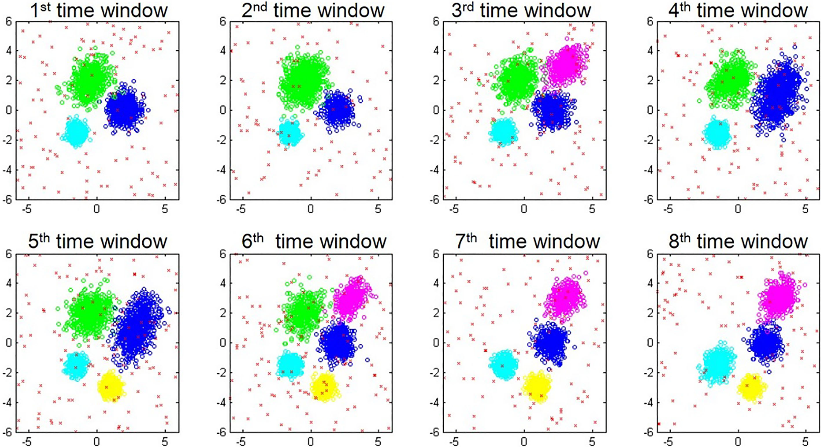

We set the pFDR level to 0.01, 0.05, 0.1, and 0.15 for the proposed method. For comparison, we also apply DenStream, which is a popular density-based data stream clustering method. We repeat the process 10 times to calculate the validation measures.

Although the results are not reported here, the estimated mean vector and covariance matrix for each cluster are very close to the true values even when the proportion of noise is high. Figure 2 shows the results obtained by the proposed method (when pFDR level is 0.1 and the fade rate is 0.9) when applied to a synthetic dataset with 5% noise points, and Fig. 3 shows the cluster results obtained by DenStream with $\epsilon=$ 3.0 and $\mu=$ 0.2.

Figure 2.

Clustering result by the proposed method when pFDR level is 0.1 for two-dimensional synthetic data with 5% noise.

Figure 3.

Clustering result by DenStream for two-dimensional synthetic data with 5% noise.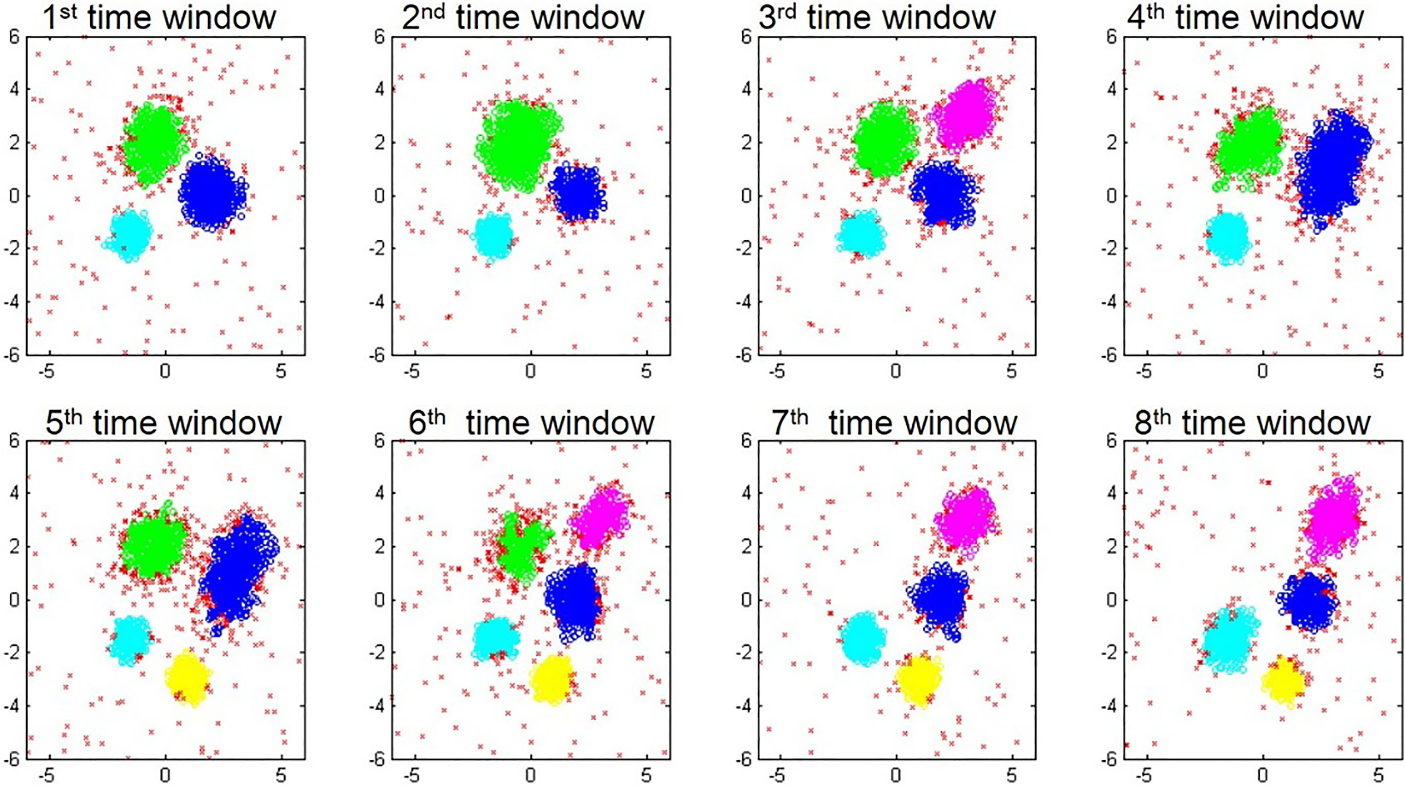

The number of clusters at the third, fifth, and seventh time windows is four; however, each distribution is quite different, as shown in Fig. 1. As can be seen in Fig. 2, the proposed method identifies clusters better than DenStream (Fig. 3) when comparing with the generated data sets.

Tables 2 and 3 show the adjusted Rand index and the mean purity, respectively, of the cluster results obtained by the proposed method and DenStream. Here, the pFDR level and fade rate used for the proposed method are 0.1 and 0.9, respectively.

Table 2

Adjusted Rand index of cluster result for two-dimensional synthetic data with 15% noise

	TW1	TW2	TW3	TW4	TW5	TW6	TW7	TW8
Proposed	0.908	0.932	0.922	0.941	0.929	0.872	0.910	0.940
DenStream	0.749	0.612	0.579	0.902	0.878	0.698	0.895	0.851

Table 3

Mean purity of cluster result for two-dimensional synthetic data with 15% noise

	TW1	TW2	TW3	TW4	TW5	TW6	TW7	TW8
Proposed	0.952	0.969	0.961	0.969	0.964	0.926	0.936	0.970
DenStream	0.837	0.800	0.693	0.948	0.939	0.791	0.935	0.915

It is clear that the proposed method provides better cluster results than DenStream in terms of adjusted Rand index and mean purity. Although the results are not reported here, these performance measures for the proposed method do not vary significantly as the pFDR level changes. However, for the proposed method, the adjusted Rand index appears to decrease and mean purity increases as the pFDR level increases because the actual cluster members tend to be declared as noise as the pFDR level increases.

Table 4 shows the actual pFDR from the proposed method according to the pFDR level (fade rate is fixed at 0.9). The results indicate that the actual pFDR values are generally less than the specified pFDR levels; however, it appears that the proposed method controls the pFDR fairly well.

Table 4

Actual FDR of the proposed method for two-dimensional synthetic data with 15% noise

pFDR level	TW1	TW2	TW3	TW4	TW5	TW6	TW7	TW8
0.01	0.010	0.010	0.005	0.006	0.006	0.003	0.003	0.003
0.05	0.038	0.042	0.029	0.034	0.028	0.014	0.015	0.023
0.1	0.071	0.088	0.065	0.071	0.066	0.034	0.041	0.053
0.15	0.106	0.135	0.097	0.104	0.092	0.060	0.070	0.089

4.2.2 Higher dimensional synthetic datasets

To observe the performance of the proposed method with higher dimensional data, we generated two more synthetic datasets with five and ten dimensions. Here, each dataset has 20 time windows. Two to five clusters are randomly selected at the first time window. Then, the number of clusters at the following time window decreases by one with a probability of 0.2, remains the same with a probability of 0.4, increases by one with a probability of 0.2, or increases by two with a probability of 0.2. The members of each cluster are generated from a multivariate normal distribution with the identity matrix for the covariance matrix. The mean of each dimensional variable is selected randomly from the set {U ( $-$ 18, $-$ 16), U ( $-$ 16, $-$ 14), …, U (16, 18), U (18, 20)}, where U (a ${}_{1}$ , a ${}_{2}$ ) is a uniform distribution with boundaries a ${}_{1}$ and a ${}_{2}$ . The number of points in each cluster is selected randomly from the set {400, 500, 600, 700}. The three cases for the proportion of noise points are 5%, 10%, and 15%.

Table 5 shows the clustering performance of the proposed method for the five-dimensional datasets with three noise cases (N5%, N10%, and N15%) according to various pFDR levels (fade rate is fixed at 0.9), as well as various fade rates (pFDR level is fixed at 0.1). Table 6 shows the results for the ten-dimensional datasets with three noise cases. They clearly show that the proposed method works well for a higher dimensional data sets regardless of the proportion of noise data points.

Table 5
Clustering performance of the proposed method for five-dimensional data sets

		Adjusted rand index			Mean purity
		N5%	N10%	N15%	N5%	N10%	N15%
pFDR	0.01	0.989	0.791	0.713	0.973	0.803	0.749
	0.05	0.988	0.704	0.591	0.990	0.725	0.665
	0.1	0.988	0.690	0.680	0.989	0.702	0.743
	0.15	0.999	0.725	0.584	0.988	0.734	0.661
Fade rate	0.7	0.987	0.637	0.535	0.987	0.638	0.601
	0.8	0.986	0.876	0.851	0.991	0.884	0.874
	0.9	0.988	0.837	0.917	0.990	0.863	0.937
	0.99	0.987	0.837	0.686	0.989	0.863	0.723

Table 6

Clustering performance of the proposed method for ten-dimensional data sets

		Adjusted rand index			Mean purity
		N5%	N10%	N15%	N 5%	N 10%	N 15%
pFDR	0.01	0.935	0.697	0.716	0.940	0.727	0.756
	0.05	0.914	0.736	0.887	0.938	0.752	0.902
	0.1	0.908	0.686	0.964	0.933	0.701	0.968
	0.15	0.936	0.838	0.883	0.950	0.874	0.899
Fade rate	0.7	0.913	0.777	0.997	0.926	0.787	0.998
	0.8	0.901	0.564	0.611	0.910	0.580	0.689
	0.9	0.858	0.825	0.854	0.892	0.858	0.866
	0.99	0.918	0.777	0.918	0.940	0.788	0.942

4.3 Real data

To demonstrate the proposed method, we use two real datasets from the UCI repository.

4.3.1 Forest cover type data

This dataset is about forest cover types, including wilderness areas located in the Roosevelt National Forest of northern Colorado, which was analyzed by Blackard and Dean [3]. The total number of data points is 581,012 in seven cover types, where type 1 comprises 36.5% of the dataset, type 2 comprises 48.8%, and other types comprise 14.7%. Each data point has 54 attributes, among which 10 are continuous attributes and 44 are binary attributes. Note that we only use the 10 continuous attributes in this study. We transform this dataset to a data stream with time windows. We divide the dataset into 117 time windows in the order of observations, each of which has 5,000 data points (the last window contains 1,012 data points). Figure 4 shows the proportions of cover types over the time windows. Types 1 and 2 primarily appear at earlier time windows and other types appear after the middle time windows.

Figure 4.

Proportions of cover types over time windows in forest cover type data.

Figure 5.

Mean purity of cluster results for forest cover type data.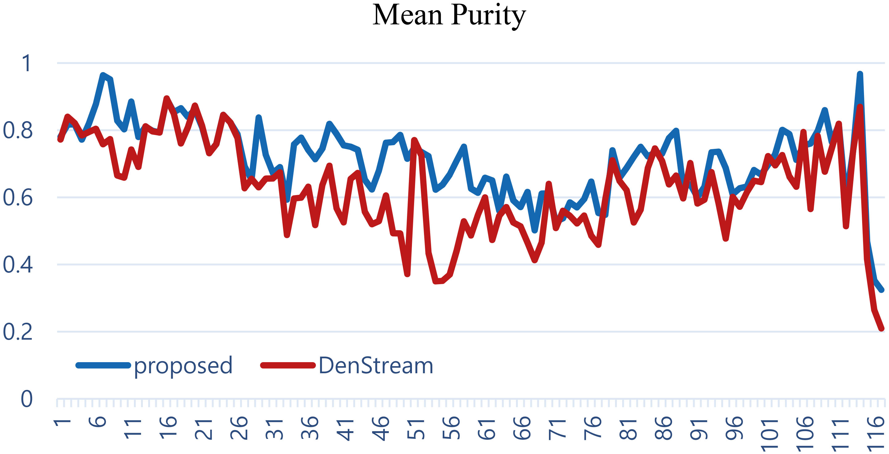

Figure 6.

Adjusted rand index of cluster results for forest cover type data.

When applying the proposed method, we set the pFDR level to 0.01 and fade rate to 0.9. For DenStream, we use $\epsilon=$ 1.4 and $\mu=$ 1. Figure 5 shows the mean purity of each time window obtained by the proposed method and DenStream. Figure 6 shows the adjusted Rand index of each time window. As can be seen, the proposed method outperforms DenStream.

4.3.2 Gas sensor array under dynamic gas mixtures data

This dataset is time series data from 16 chemical sensors exposed to gas mixtures under various mixing ratios, which was analyzed by Fonollosa et al. [12]. There are two gas mixtures, i.e., ethylene and methane in air, and ethylene and CO in air. Note that we selected a set of ethylene and CO in air. The total number of data points is 4,208,261. There are 73 different types of mixing ratios. Among them, we use 1,000,000 data points in 41 different mixing ratios. The number of type 1 data points is 24%, and the ratios of other types are less than 7%. There are 16 attributes from the sensors for each data point. We transform the dataset to a data stream with 5,000 data points at each time window such that there are 200 time windows. Table 7 shows the number of types and the major types at selected time windows. As can be seen, most time windows contain only one type; however, the major type changes over the time windows.

Table 7
The numbers of types and the major types at selected time windows in gas sensor array data

Time window	TW ${}_{1}$	TW ${}_{2}$	TW ${}_{3}$	TW ${}_{4}$	TW ${}_{5}$	TW ${}_{6}$	TW ${}_{7}$	TW ${}_{8}$	TW ${}_{9}$	TW ${}_{10}$
# types	1	2	1	2	1	2	1	1	1	2
Major type	1	1	2	2	3	3	1	1	1	1
Time window	TW ${}_{111}$	TW ${}_{112}$	TW ${}_{113}$	TW ${}_{114}$	TW ${}_{115}$	TW ${}_{116}$	TW ${}_{117}$	TW ${}_{118}$	TW ${}_{119}$	TW ${}_{120}$
# types	1	1	1	3	1	2	1	1	1	2
Major type	17	17	17	17	5	5	1	1	1	1
Time window	TW ${}_{191}$	TW ${}_{192}$	TW ${}_{193}$	TW ${}_{194}$	TW ${}_{195}$	TW ${}_{196}$	TW ${}_{197}$	TW ${}_{198}$	TW ${}_{199}$	TW ${}_{200}$
# types	1	2	1	2	2	1	2	1	2	1
Major type	22	27	27	40	40	22	22	27	41	41

For this dataset, we set the pFDR level to 0.01 and fade rate to 0.9 for the proposed method. Figure 7 shows the mean purity of the cluster results at 43 selected time windows. We selected time windows that contains at least two types of gas mixtures and whose major type is at most 80%. The maximum proportion represents the estimated proportion of the major type. Note that the clustering results have the same or higher purity than the maximum proportion. Figure 8 shows the adjusted Rand index of the cluster results for the selected time windows. The bar chart indicates the number of clusters found at each time window. The Rand index tends to be lower if the number of clusters is larger due to the imbalanced distribution of mixture types. Generally, the proposed method shows good performance in terms of these measures.

Figure 7.

Mean purities over selected time windows by the proposed method for gas sensor array data.

Figure 8.

Adjusted Rand indices over selected time windows by the proposed method for gas sensor array data.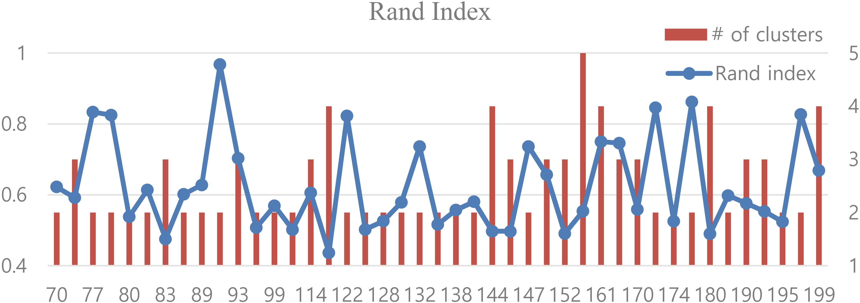

We also attempted to apply DenStream to this dataset; however, it turned out that all data points were determined as a single cluster or noise at each time window.

5. Conclusion

In this study, a hybrid data steam clustering method that combines model-based and density-based clustering is proposed. The performance of the proposed method is evaluated in terms of mean purity and the adjusted rand index. Experiments with synthetic datasets and two real datasets show that the proposed method responds quickly to cluster evolution and detects noise quite well by controlling the decision error of the pFDR near a predefined level. Compared to DenStream, the proposed method shows better and more robust performance.

As observed from the experimental results obtained with higher dimensional datasets, the performance of the proposed method may degrade as dimension increases. Therefore, suitable dimension reduction is recommended for this clustering procedure. Note that the two real datasets are not originally data streams; however, these datasets were transformed to data streams. This shows the possibility of handling and analyzing big data by transforming it into a data stream with time windows.

The analysis of big data with the aid of data stream clustering may be an interesting problem, which should be further studied in a future research. Also, missing values in some variables are present frequently in a real data set, so the handling missing values in a data stream algorithm can be included in a future study.

Footnotes

Acknowledgments

This work was supported by the National Research Foundation of Korea (NRF) grant funded by the Korea Government MEST (No 2017R1A2B4005450).

Appendix Pseudo code of the proposed algorithm

Proposed algorithm
Input: Dataset $X$ , radius $\epsilon$ , Minimum number of points MinPts-1, 2, min_cluster_num, desired number of clusters $K$ ,
p-threshold $\lambda$ , cluster-threshold $q^{*}$
Initial Phase
1. Separate Non_noise_data and Noise_data by using DBSCAN (X, $\epsilon$ , MinPts-1)
2. Update cluster information $(\mu_{k}),(\Sigma_{k}),K$ by using incremental EM based on BIC
3. Compute $p$ -value $p_{i}$ of each data points in Eq. (3)
4. If $\text{pFDR}(x_{i},\lambda)=\frac{\#\{p_{j}>\lambda\}\cdot p_{i}}{(1-\lambda)% \text{max}[1,\#(p_{j}<p_{i})]}<q^{*}$ , then $x_{i}$ is a noise data
5. Else, $x_{i}$ is a cluster member of $c_{i}={\text{argmax}}_{\text{k}}w_{ik}$ where $w_{ik}=\frac{n_{k}(x_{i}\|{\mu}_{k},\Sigma_{k})\cdot\alpha_{k}}{\sum^{K}_{m=1}n% _{m}(x_{i}\|{\mu}_{m},{{\Sigma}}_{m})\cdot\alpha_{m}}$
Incremental Phase
6. For new data points at $t$ -th time window, (use notations in Section 3.4)
7. Compute $p$ -values for each component of the GMM $p_{ik}(i=1,\dots,N^{t},k=1,\dots K^{t-1})$
8. Calculate proportion of cluster members $w_{k}(\lambda)=\min\left\{1,\frac{\#\left\{p_{ik}>\lambda\right\}}{\left(1-% \lambda\right)N^{t}}\right\}$ for $k=1,\dots,K^{t-1}$
9. For each cluster, assign top- $w_{k}(\lambda)\times N^{t}$ data points in terms of $p$ -values
10. Data points assigned to two or more clusters, randomly select one cluster and unassigned data points are classified as
temporarily noise points
11. $D^{\textit{new}}_{i}$ for $i=1,\ldots,K^{\textit{new}}$ is new clustering result from DBSCAN on temporarily noise data
12. If $\left\|D^{\textit{new}}_{i}\right\|>$ min_cluster_num, then
13. Find the closest existing cluster $C_{c}$ to $D^{\textit{new}}_{i}$
14. Estimate BIC-1 of the Gaussian mixture model with 1 component on $x\in(C_{c}\cup D^{\textit{new}}_{i})$
15. Estimate BIC-2 of the Gaussian mixture model with 2 component on $x\in(C_{c}\cup D^{\textit{new}}_{i})$
16. If BIC-2 $<$ BIC-1, then $D^{\textit{new}}_{i}$ is declared as a new cluster, else is assigned into existing clusters
17. update cluster information $(\mu_{k})$ , $(\Sigma_{k})$ , $K$ by using incremental EM based on BIC
18. If number of members $<$ MinPts-2 for some clusters, then remove the cluster and re-allocate members in it
19. Update the cluster result using Eqs (8)–(10)
20. Separate noise data by multiple hypothesis testing (3. $\mathrm{\sim}$ 5.)

References

Aggarwal

C.C.

Han

Wang

and Yu

P.S.

, A framework for clustering evolving data streams, in: Proceedings of the 29th International Conference on Very Large Data Bases (VLDB 2003), Vol. 29, 2003, pp. 81–92.

Amini

Wah

T.Y.

and Saboohi

, On density-based data streams clustering algorithms: A survey, Journal of Computer Science and Technology 29(1) (2014), 116–141.

Blackard

J.A.

and Dean

D.J.

, Comparative accuracies of artificial neural networks and discriminant analysis in predicting forest cover types from cartographic variables, Computers and Electronics in Agriculture 24(3) (1999), 131–151.

Blekas

and Lagaris

I.E.

, Split-merge incremental learning (SMILE) of mixture models, Artificial Neural Networks – ICANN 2007, Springer Berlin Heidelberg, 2007, 291–300.

Cao

Ester

Qian

and Zhou

, Density-based clustering over an evolving data stream with noise, in: Proc. SIAM Conf. Data Mining, 2006, pp. 326–337.

Chen

J.-Y.

and He

H.-H.

, A fast density-based data stream clustering algorithm with cluster centers self-determined for mixed data, Information Sciences 345 (2016), 271–293.

Dang

X.H.

Lee

W.K.

Ciptadi

and Ong

K.L.

, An EM-based algorithm for clustering data streams in sliding windows, in: Zhou

et al. (eds), Database Systems for Advanced Applications. DASFAA 2009, Lecture Notes in Computer Science, Vol. 5463, 2009, Springer Berlin Heidelberg.

Daszykowski

Walczak

and Massart

D.L.

, Looking for natural patterns in data: Part 1. density-based approach, Chemometrics and Intelligent Laboratory Systems 56(2) (2001), 83–92.

Dempster

A.P.

Laird

N.M.

and Rubin

D.B.

, Maximum likelihood from incomplete data via the EM algorithm, Journal of the Royal Statistical Society. Series B 39(1) (1977), 1–38.

10.

Ding

Zhang

Jia

and Qian

, An adaptive density data stream clustering, Cognitive Computation 8(1) (2016), 30–38.

11.

Ester

Kriegel

H.-P.

Sander

and Xu

, A density-based algorithm for discovering clusters in large spatial databases with noise, in: Proceedings of the Second International Conference on Knowledge Discovery and Data Mining (KDD 1996), AAAI, 1996, pp. 226–231.

12.

Fonollosa

Sheik

Huerta

and Marco

, Reservoir computing compensates slow response of chemosensor arrays exposed to fast varying gas concentrations in continuous monitoring, Sensors and Actuators B: Chemical 215 (2015), 618–629.

13.

Handl

Knowles

and Kell

, Computational cluster validation in post-genomic data analysis, Bioinformatics 21 (2005), 3201–3212.

14.

Hua

and Mou

, A data stream clustering algorithm based on density and extended grid, in: Huang

D.S.

K.H.

and Figueroa-García

(eds), Intelligent Computing Theories and Application. ICIC 2017. Lecture Notes in Computer Science, Vol. 10362, 2017, Springer, pp. 689–699.

15.

Hubert

and Arabie

, Comparing partitions, Journal of Classification 2(1) (1985), 193–218.

16.

Kaufman

and Rousseeuw

P.J.

, Finding groups in data: An introduction to cluster analysis, Wiley, New York, 1990.

17.

Kranen

Assent

Baldauf

and Seidl

, The ClusTree: indexing micro-clusters for anytime stream mining, Knowledge and Information Systems 29(2) (2011), 249–272.

18.

Lee

and Jun

C.-H.

, PCA-based high-dimensional noisy data clustering via control of decision errors, Knowledge-Based Systems 37 (2013), 338–345.

19.

Mattern

and Flörkemeier

, From the internet of computers to the internet of things, in: Sachs

Petrov

and Guerrero

(Eds), From Active Data Management to Event-Based Systems and More, Lecture Notes in Computer Science, Vol. 6462, 2010, Springer, Berlin, pp. 242–259.

20.

Nguyen

Woon

Y.-K.

and Ng

W.-K.

, A survey on data stream clustering and classification, Knowledge and Information Systems 45(3) (2015), 535–569.

21.

Park

H.-S.

Lee

and Jun

C.-H.

, Clustering noise-included data by controlling decision errors, Annals of Operations Research 216(1) (2014), 129–144.

22.

Rand

W.M.

, Objective criteria for the evaluation of clustering methods, Journal of the American Statistical Association 66(336) (1971), 846–850.

23.

Schwarz

, Estimating the dimension of a model, The Annals of Statistics 6(2) (1978), 461–464.

24.

Song

and Wang

, Highly efficient incremental estimation of Gaussian mixture models for online data stream clustering, in: Proceedings of SPIE Conference on Intelligent Computing: Theory and Applications III, 2005.

25.

Storey

J.D.

, The positive false discovery rate: a Bayesian interpretation and the q-value, The Annals of Statistics 31 (2003), 2013–2035.

26.

and Chen

, Stream data clustering based on grid density and attraction, ACM Transactions on Knowledge Discovery from Data (TKDD) 3(3) (2009), 1–26.

27.

Ueda

Nakano

Ghahramani

and Hinton

G.E.

, SMEM algorithm for mixture models, Neural Computation 12(9) (2000), 2109–2128.

28.