Multi-view deep unsupervised transfer leaning via joint auto-encoder coupled with dictionary learning

Abstract

Transfer learning empowers machine learning algorithms the ability to train a model on a given task, capture the existing relationship in the data and reuse it for another task in the same or similar domain. In this paper, we present a Multi-view deep unsupervised transfer leaning via joint auto-encoder coupled with dictionary learning (MVT-DAE). In the proposed approach knowledge transfer is done in two stages. First, we perform multi-view dictionary learning based on low-rank tensor regularization in the source domain to learn the common intrinsic relationship among views. Then we transfer the learned dictionaries to the target domain, and we construct a new representation of both domain via sparse coding. In the second stage, we use two deep auto-encoders (DAE) from both sources to perform parameters transfer. Each DAE consist of an embedding layer and a label layer. The embedding layer reconstructs the input while the label layer is used to encode the label information. To relax the distribution distance of the embedding and label layer between the source and the target domain a joint maximum mean discrepancy (JMMD) is employed. Learning can be done via Stochastic gradient descent by sharing the embedding and label layer weights with the target domain. We conduct extensive experiments in two real-world datasets which demonstrated the effectiveness of our approach compared with the different state of the art baseline.

Keywords

Transfer learning multi-view deep auto-encoder dictionary learning

1. Introduction

Deep learning has lifted the state of the art of machine learning significantly to an entirely different level. However, to build a model with high performance using deep neural network a tremendous amount of label data is required. In many real-world applications it is very difficult almost entirely impossible to get enough and labeled dataset, and manually label data from diverse applications is often prohibited. For instance, in urban computing, we might need to predict the Air quality index in some cities. In well-developed cities, the data needed to conduct such a task might be straightforward to get, but if we move to less developed cities in which infrastructures and services are less advanced, the task becomes more challenging due to the insufficiency of available data. Another example is classifying medical image scan to detect potential disease. Some images might be tough to get due to the rarity of the underlying disease. Transfer learning comes to rescue by capturing the relationship existing in a particular data type from one task and reuse it to another task in a same or similar domain [18]. However, this learning paradigm suffers from a significant issue which is the distribution shift between domains thus causes considerable challenge when we use the predictive model to the target task.

Transfer learning becomes more challenge in a multi-view or multi-source setting. Many machine learning applications required data from diverse source to reach a satisfactory performance. Although there are many transfer learning approaches, dealing with multiple sources or views [8, 25, 26], there are only a few attempts that tackle the challenging problem when both source and target are represented by multi-view data. Going back to the urban computing example, predicting the air quality index required data from a diverse source, e.g., air quality data, meteorological data, point of interest (POI), weather forecast, etc $\ldots$ A naïve approach would be to concatenate those different views and apply existing transfer learning approach. This will, of course, compromises the predictive model as some views have a different representation, e.g., POI is represented as Boolean values whereas meteorological is represented as real values. Performing transfer learning on image dataset may involve in some application multi-view features for better performance .e.g. we can extract deep features using standard Convolution neural network (CNN). However, some features are not always transferrable for some application. Taking the AlexNet [2] as an example, the literature said the higher fully connected layers (fc6, fc7, fc8) are not always transferable for domain adaption [10]. Thus employing multi-view source features from multiple CNN to perform knowledge transfer to a multi-view target can indeed improve the performance of the underlining task.

In this paper, we proposed a multi-view deep unsupervised transfer leaning via joint auto-encoder coupled with dictionary learning (MVT-DAE). MVT-DAE extends the ability of deep auto-encoders to reason about the multi-view transfer learning challenges as mentioned above. The proposed approach performs in two stages. At the first stage, a multi-view dictionary learning based on low-rank tensor is performed at the source domain only. Indeed views might be very different, but they can share some intrinsic cooperation. Thus it becomes crucial to learn a new enriched representation of each view so that the universal relation is present in each view. We learn this new representation by performing sparse coding using the resulting dictionaries. We transfer the dictionaries to the target domain, and we also learn a new enriched representation for the target domain views. In this way, we ensure each view in both source and target is well representative of the underlying context. At the second stage of MVT-DAE, we conduct parameters transfer via deep auto-encoder (DAE). We construct a DAE for both source and target, each consisting of an embedding and label layer. The embedding layer reconstructs the input views whereas the label layer encodes the label information. To enforce the distribution gap between the source and target, we minimize the join maximum mean discrepancy primarily introduced in [14].

One major challenge when dealing with multi-view transfer learning is how to handle missing observation in the target domain when some observations in some views are missing, and in some particular cases, the whole view might be absent. In previous transfer learning approach, missing value is treated as a latent factor and recovered by introducing a low-rank constraint [18, 22, 24, 26]. This approach is only applicable on one view to one view transfer setting. In our approach, we use a Max-pooling to deal with missing observation. Max-pooling commonly used in many computer vision applications aggregates each target instance of all existing view into one so that the target instance can be treated equally regardless of the missing views.

In summary, the main contributions of the proposed method are three-fold: 1) A multi-view dictionary learning approach is proposed to lean an enriched representation of the source domain and target domain. 2) Joint deep auto-encoder which incorporates a label layer to encode the label information and constrained with join maximum mean discrepancy to combat the distribution shift between the two domains. 3) We evaluate our method using on two real-world datasets, an urban dataset to predict air quality index and an image dataset for images classification.

2. Related work

In this section, we review the recent related work in two transfer learning research: Transfer learning from multi-source and transfer learning via deep auto-encoder

2.1 Transfer learning from multi-source

There have been many attempts in performing transfer learning from multi-source data. Most of them are only applicable when the target domain can be represented in the single view. Ding et al.[25, 26] propose a multi-source transfer learning through bi-directional low rank [9, 23] transfer. In this approach, a cross-source regularization is added to couple the same label from a different source to compensate missing observations.

Zhuang et al. [8] come up with a new multi-source transfer learning method with consensus regularization. Individually multiple classifiers from multiple sources jointly perform an entropy-based consensus regularization on the target domain prediction [6, 17]. All of those approaches suppose the target domain can be represented by a single view.

Recently a Flexible multi-model transfer learning method (FLORAL) [18] was proposed to transfer knowledge from source city to a target city where each city is represented by multi-modal datasets, e.g., POI, taxi trajectories, AQI dataset, etc. FLORAL learns some semantically related dictionary from the source and simultaneously transfer dictionary and instance to the target domain. However, FLORAL performs in a semi-supervised fashion as it requires some label data from the target domain to perform knowledge transfer. The DISMUTE method proposed in [27] can efficiently perform a transfer from a multi-view source domain to multi-view target domain by conducting a sparse features selection and at the same time minimize the distribution gap between the domains via maximum mean discrepancy (MMD) [1] regularization. However, this approach does not treat missing view for some observation thus make it less efficient in a real world where data insufficiency is a real issue.

2.2 Transfer learning via deep auto-encoder

Because of its ability to learn high-level features, deep learning has recently been applied to transfer learning [4, 7, 15, 19, 20, 23]. The most common technique is called fine-tuning, where we extract features from a pre-trained model and a fully connected deep neural network is used to conduct training. Such a technique is only applicable in a situation where we dispose of fully labeled but limited target data. Recent research has demonstrated the ability to use deep auto-encoder to perform knowledge transfer to the unlabeled target domain. In [10] the authors propose a transfer learning based on deep auto-encoder in three step: 1) all the encoding and decoding weights are shared by the source and the target, 2) enforce the closeness of the distribution between the embedding layers of the source and target via KL-Divergence. 3) encodes the label information with softmax regression. However, this approach naively transfer all the weights to the target which make it less efficient in a more complicated target domain. To leverage this issues Moon and Carbonell propose CHTL in [14] a more efficient approach with attention to what and what not to transfer. CHTL construct a denoising auto-encoder [16] to select a subset of source sample to transfer from, and build a join embedded subspace and ensure only the weight on that subspace are shared. To best of our knowledge, there is no attempt of using DAE for transfer learning in which the source and the target domain are all represented by multi-view data.

In this paper, we come up with a novel unsupervised multi-view transfer learning based on deep auto-encoder empowered with a Joint Maximum Mean Discrepancy that can leverage the wealth of information from multi-view source domain to perform knowledge transfer to an insufficient and unlabeled multi-view target domain.

3. Proposed approach

3.1 Problem definition

Suppose we dispose of multiple labeled data in a source domains from K independent views, $X_{v}^{s}=\{{x_{v,1}^{s},x_{v,2}^{s},\ldots,x_{v,N_{s}}^{s}}\}\in R^{d_{v}\ast N% _{s}}v=1\ldots$ K. $d_{v}$ is the dimensionality of the $v^{th}$ view in the source domain $D^{s}$ and $N_{s}$ represent the number of instance of the view $X_{v}^{s}$ . We define $Y^{s}=\{{y_{1}^{s},y_{2}^{s},\ldots,y_{N_{s}}^{s}}\}$ where $y_{i}^{s}\in\{{0,1}\}^{c\times 1}$ the corresponding label for the data instance $\{{X_{v,i}^{s}}\}_{v=1}^{K}$ and c is the number of label classes. Besides the source domain data, we also dispose of unlabeled target domain data instances from K views $X_{v}^{t}=\{{x_{v,1}^{t},x_{v,2}^{t},\ldots,x_{v,N_{t}}^{t}}\}\in R^{d_{v}\ast N% _{t}}v=1\ldots$ K., $d_{v}$ is the dimensionality of $v^{th}$ views in the target domain $D^{t}$ and $N_{t}$ represent the total number of data instance in the view $X_{v}^{t}$ . Similar to the source domain we also define $Y^{t}=\{{y_{1}^{t},y_{2}^{t},\ldots,y_{N_{t}}^{t}}\}$ where $y_{i}^{t}$ represents the unknown label class for the data instance $\{{x_{v,i}^{t}}\}_{v=1}^{K}$ . With the notation given above our goal is to learn a new representation of each view in each domain and also be able to predict the class label matrix $Y^{t}$ for the target domain by taking into consideration the distribution shift between domains and the misses existing in the target domain.

3.2 Join Maximum mean discrepancy

The Maximum mean discrepancy [1] has been widely used in many transfer learning approach to measuring the marginal distribution shift between two domains $D_{X^{s}}$ and $D_{X^{t}}$ from distribution $P({X^{s}})$ and $Q({X^{t}})$ . However when applying transfer learning through deep learning it is essential to point out the join distribution between $P({X^{s},Y^{s}})$ and $Q({X^{t},Y^{t}})$ linger not only at first layer but also in the hidden layers. In our case we have an embedding and label layer in each deep auto-encoder, the features distribution shift mainly occurs at the embedding layer while the label distribution shift lingers at the label layer. So we need to find a way to surrogate the original joint distribution $P({X^{s},Y^{s}})$ and $Q({X^{t},Y^{t}})$ . To do that we employ the Join Maximum Mean discrepancy introduced by Long et al. [23]. The JMMD uses the Hilbert space embedding [13] of joint distributions to measure the discrepancy between $P({Z_{1}^{s}\ldots,Z_{L}^{s}})$ and $Q({Z_{1}^{t},\ldots,Z_{L}^{t}})$ where $Z_{L}^{s/t},\ldots,Z_{L}^{s/t}$ represent the activation of the highest layer $L$ generated by the deep network. $\textit{JMMD}_{L}({X^{s},X^{t}})$ can be computed as the square distance between all empirical Hilbert kernel mean embedding of hidden layers of the source and target domain follow as:

$\displaystyle\textit{JMMD}_{L}(X^{s},X^{t})=\frac{1}{N_{s}^{2}}\sum^{N_{s}}_{i% =1}\sum^{N_{s}}_{j=1}\prod_{l\in L}k^{l}(z^{sl}_{i},z^{sl}_{j})+\frac{1}{N^{2}% _{t}}\sum^{N_{t}}_{i=1}\sum^{N_{t}}_{j=1}\prod_{l\in L}k^{l}(z^{tl}_{i},z^{tl}% _{j})+\frac{1}{N_{s}N_{t}}\sum^{N_{s}}_{i=1}\sum^{N_{t}}_{j=1}\prod_{l\in L}k^% {l}(z^{sl}_{i},z^{tl}_{j})$

3.3 MVT-DAE overview

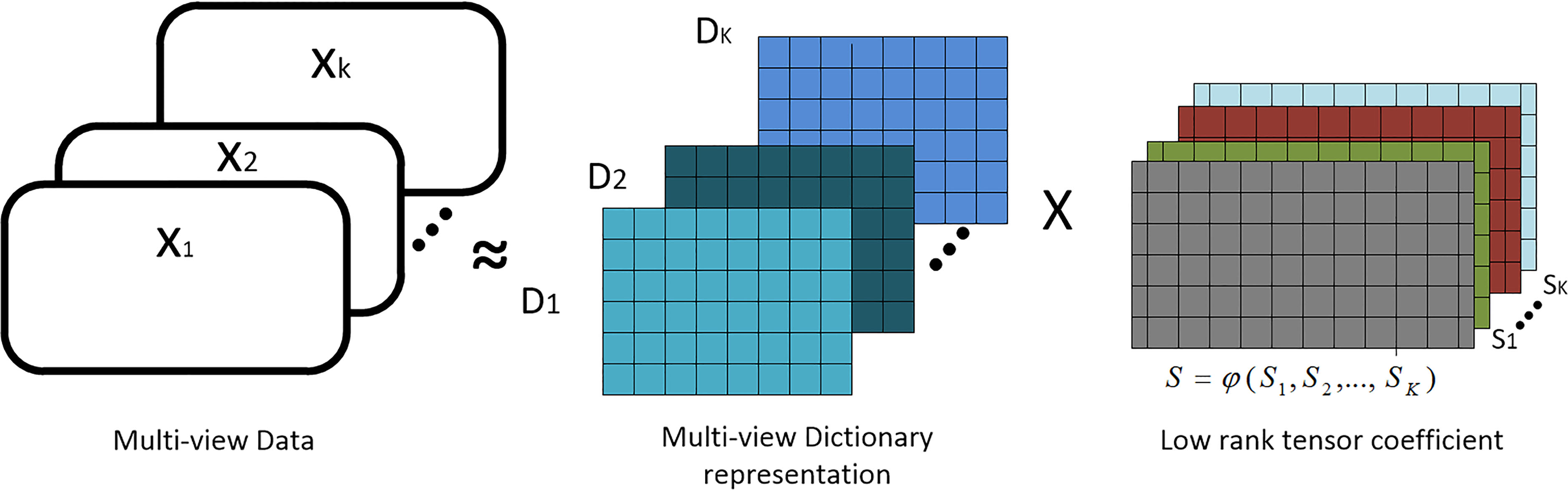
In this section, we briefly describe our multi-view deep unsupervised transfer leaning via joint auto-encoder coupled with dictionary learning approach. The general framework is introduced in Fig. 1. At first, from the source domain views $\{{X_{v}^{s}}\}_{v=1}^{K}$ we learn K dictionaries $\{{D_{v}}\}_{v=1}^{K}$ via a multi-view dictionary learning based on low-rank tensor minimization. Once the dictionaries are obtained we construct a new enriched presentation of each source domain’s views $\{\hat{X}^{s}_{v,i}\}^{K}_{v=1}$ . The dictionaries $\{{D_{v}}\}_{v=1}^{K}$ are also used to perform the first stage of the transfer. Concretely using $\{{D_{v}}\}_{v=1}^{K}$ we learn an enriched representation of each view in the target domain and then we applied max pooling to combat missing values. At the second stage of the transfer, we jointly learn two DAEs with an embedding $\sigma_{i}^{s/t}$ and label layer $z_{i}^{s/t}$ in both domains. The embedding layer reconstructs the input data and the label layer encodes the label information from the source domain. To handle the distribution shift between the domain we minimize the JDMM between the embedding and label layer of the source and target domain.

Figure 1.

Unsupervised multi-view transfer learning based on deep auto-encode.

In this way, we ensure that our transfer learning model takes great advantage from all information spread out from different views at the source but also ensure the feature and label distribution shift are minimized during the training.

3.4 Learning related dictionaries from the source domain

When dealing with multi-view data it is important to point out they are highly related to each other as they share some common intrinsic cooperation but at the same time, they can very different as well. So knowledge transfer cannot efficiently be done without deeply mining and merging the relationship existing between them. There exist three types of data fusion method: stage-based data fusion, feature level-based data fusion and semantic meaning based data fusion, multi-view learning falls into the former one. Knowledge transfer can easily be improved via multi-view representation as it can capture a rich and complementary information hidden among different views. In our framework, to explore the complementary information between views, we formulate a multi-view dictionary learning task in the source domain only by introducing a regularized dictionary learning via a low-rank tensor. The low-rank tensor can indeed learn the cross information existing among views by capturing the high order correlations among them as follows:

$\displaystyle\textit{min}_{D_{v},S_{v}}\mathop{\sum}\limits_{i=1}^{K}||X_{v}^{% s}-D_{v}S_{v}||_{F}^{2}+||S||_{\ast}$ $\displaystyle\quad\textit{with}\ ||S||_{\ast}=\mathop{\sum}\limits_{m=1}^{M}% \varepsilon_{m}||S^{(m)}||_{\ast}$ (1) $\displaystyle\quad\textit{St.S}=\varphi\left({S_{1},S_{2},\ldots,S_{K}}\right)$

Figure 2.

Multi-view dictionary learning based on low rank tensor.

The Fig. 2 describes the multi-view dictionary learning in more details. Note the difference between $S_{v}$ and $S^{(m)}$ . $S_{v}\in R^{Q\ast N_{s}}$ represents the coding coefficient associated to the vth view, while $S^{\left(m\right)}$ represents the m-mode unfolding matrix of the tensor $S$ . The function $\varphi\left(\ast\right)$ will construct the tensor $S$ by merging the $S_{v}$ to a 3-order tensor with dimensionality $Q\times N_{s}\times K$ , with $Q$ the common dimensionality of the dictionary $D_{v}$ . The problem Eq. (3.4) can be solved by introducing an auxiliary variable $T_{m}$ as in [3].

$\displaystyle\textit{min}_{D_{v},S_{v},T_{m}}\mathop{\sum}\limits_{i=1}^{K}||X% _{v}^{s}-D_{v}S_{v}||_{F}^{2}+\mathop{\sum}\limits_{m=1}^{M}\varepsilon_{m}||T% _{m}||_{\ast}$ $\displaystyle\quad\textit{St.S}=\varphi\left({S_{1},S_{2},\ldots,S_{M}}\right)$ (2) $\displaystyle\quad R_{m}s=t_{m}\ \text{and}\ m=1,2,\ldots,M$

Where $s$ and $t_{m}$ represent respectively the vectorization of S and $T_{m}$ . $R_{m}$ matrix is used to align the corresponding elements between $S^{(m)}$ . and $T_{m}$ . Using the Alternating Lagrange Multiplier (ALM) optimization algorithm Eq. (3.4) can be solved by minimizing the following augmented Lagrangian function.

$\displaystyle\text{H}=\mathop{\sum}\limits_{v=1}^{K}||X_{v}^{s}-D_{v}S_{v}||_{% F}^{2}+\mathop{\sum}\limits_{m=1}^{M}\left({\varepsilon_{m}||T_{m}||_{\ast}+% \frac{\mu}{2}\left({\left|\left|R_{m}s-t_{m}+\frac{\alpha_{m}}{\mu}\right|% \right|_{F}^{2}}\right)}\right)$

3.4.1 Update

S_{v}

To update the coding coefficient of $S_{v}$ for the v-th view we fix the other variables and solve the following optimization problem:

$\displaystyle\text{min}_{S_{v}}\text{{H}}\left({S_{v}}\right)=||X_{v}^{s}-D_{v% }S_{v}||_{F}^{2}+\mathop{\sum}\limits_{m=1}^{M}\frac{\mu}{2}\left({\left|\left% |R_{m}s-t_{m}+\frac{\alpha_{m}}{\mu}\right|\right|_{F}^{2}}\right)$

Knowing that s represent the vectorization of the tensor $S$ , when updating $S_{v}$ we only need to select its corresponding value within the vector $s$ . To do so, we define the function $\Omega^{v}(a)$ which select only the $Q\times N_{s}$ elements corresponding to $S_{v}$ and turn it into $Q\times N_{s}$ matrix. Thus $S_{v}$ can be updated as follows:

$\displaystyle\text{min}_{S_{v}}{H}\left(S_{v}\right)=||X_{v}^{s}-D_{v}S_{v}||_% {F}^{2}+\mathop{\sum}\limits_{m=1}^{M}\frac{\mu}{2}\left(\left|\left|\Omega^{v% }\left(R_{m}s+\frac{\alpha_{m}}{\mu}\right)-\Omega^{v}(t_{m})\right|\right|_{F% }^{2}\right)$

The closed form of $S_{v}$ can then be computed as follows:

$\displaystyle S_{v}=\left({D_{v}D_{v}^{T}+\textit{MI}}\right)^{-1}\times\left(% {\mathop{\sum}\limits_{m=1}^{M}{\Omega}^{v}\left({t_{m}}\right)-\mathop{\sum}% \limits_{m=1}^{M}{\Omega}^{v}\left({\frac{\alpha_{m}}{\mu}}\right)+D_{v}^{T}X_% {v}^{s}}\right)$

3.4.2 Update $D_{v}$

$D_{v}$ can easily be updated by solving the following optimization problem: $\text{min}_{D_{v}}{{\rm H}}\left({D_{v}}\right)=||X_{v}^{s}-D_{v}S_{v}||_{F}^{2}$ .

The closed form of $D_{v}$ can then be computed as follows: $D_{v}=X_{v}^{s}S_{v}^{T}({S_{v}S_{v}^{T}})^{-1}$ .

3.4.3 Update $T_{m}$

We can update $T_{m}$ by solving the following optimization problem:

$\displaystyle\text{min}_{T_{m}}{{\rm H}}\left({T_{m}}\right)=\varepsilon_{m}||% T_{m}||_{\ast}+\frac{\mu}{2}\left({\left|\left|R_{m}s-t_{m}+\frac{\alpha_{m}}{% \mu}\right|\right|_{F}^{2}}\right)$

To solve this problem, we need to introduce a function $\Omega^{m}(a)$ that reshape the vector a to a matrix corresponding to an m-mode unfolding; thus previous equation then became :

$\displaystyle\text{min}_{T_{m}}\text{H}(T_{m})=\varepsilon_{m}||T_{m}||_{\ast}% +\frac{\mu}{2}\left(\left|\left|\Omega^{m}\left(R_{m}s+\frac{\alpha_{m}}{\mu}% \right)-{\Omega}^{m}\left({t_{m}}\right)\right|\right|_{F}^{2}\right)$

This equation can be solved via using the Single value threshold (SVT) method, and $T_{m}$ can be computed as follows:

$\displaystyle T_{m}=\textit{Proxy}_{\frac{\varepsilon_{m}}{\mu}}^{tr}\left({{% \Omega}^{m}\left({R_{m}s+\alpha_{m}}\right)}\right)$

Where $\frac{\varepsilon_{m}}{\mu}$ denote the threshold of the spectral soft-threshold operation $\textit{Proxy}_{\frac{\varepsilon_{m}}{\mu}}^{tr}\left(L\right)=U.\max$ $({S-\frac{\varepsilon_{m}}{\mu},0}).V^{t}$ with $L=\textit{USV}^{t}$ being the single value decomposition (SVD) of the matrix L.

The Algorithm 1 is a description of the overall optimization procedure of H function.

Algorithm 1: Learning an enriched representation of the source domain
Input: $\left\{{X_{v}^{s}}\right\}_{v=1}^{K}$
$\Omega^{m}\left(a\right)$ : Function that reshapes the vector a to matrix corresponding to m-mode unfolding
$\Omega^{v}\left(a\right)$ : Function that only selects $Q\times N_{s}$ elements of the vector a and turns it into a $Q\times N_{s}$ matrix
Output: $S_{v}$ , $D_{v}$
1. While not converge iter $<=$ maxIter do
2. for $v$ : 1 to K
3. $S_{v}=\left({D_{v}D_{v}^{T}+\textit{MI}}\right)^{-1}\times\left({\mathop{\sum}% \limits_{m=1}^{M}{\Omega}^{v}\left({t_{m}}\right)-\mathop{\sum}\limits_{m=1}^{% M}{\Omega}^{v}\left({\frac{\alpha_{m}}{\mu}}\right)+D_{v}^{T}X_{v}^{s}}\right)$
4. $s=S_{v}$ // we replace the corresponding elements
5. $D_{v}=X_{v}^{s}S_{v}^{T}\left({S_{v}S_{v}^{T}}\right)^{-1}$
6. end
7. for $m=$ 1 to M
8. $T_{m}=\textit{Proxy}_{\frac{\varepsilon_{m}}{\mu}}^{tr}\left({{\Omega}^{m}% \left({R_{m}s+\alpha_{m}}\right)}\right)$
9. $t_{m}=T_{m}$ // we replace the corresponding elements
10. $\alpha_{m}=\alpha_{m}+\left({R_{m}s-t_{m}}\right)$
11. end
12. check the convergence:
13. $\|\|X_{v}^{s}-D_{v}S_{v}\|\|_{\textit{inf}}<\textit{eps}$
14. $\|\|R_{m}s-t_{m}\|\|_{\textit{inf}}<\textit{eps}$
15. Return $S_{v}$ , $D_{v}$

The Algorithm 1 learns K related dictionary by homogenizing different views, $\{{D_{v}}\}_{v=1}^{K}$ , and the coding coefficients matrix $\{{S_{v}}\}_{v=1}^{K}$ . The new enriched representation of each view in the source domain data can be constructed via sparse coding as follows:

$\displaystyle\textit{min}_{\widehat{X_{v,i}^{s}}}||X_{v,i}^{s}-D_{v}\hat{X}^{S% }_{v,i}||^{2}_{F}+\alpha||\hat{X}^{S}_{v,i}||_{1}$

This new representation $\hat{X}^{S}_{v}$ will then be used to conduct knowledge transfer from the source to the target domain. The dictionary $\{{D_{v}}\}_{v=1}^{K}$ are also transferred to the target domain to lean an enriched representation for each view in the target domain to tackle the data insufficiency issues. Concretely from the v-th view of the i-th unlabeled instance in the target domain $X_{i}^{t}$ we transfer the dictionary $D_{v}$ learned from the source domain and apply the sparse coding to construct the new enriched representation for the target data as follows:

$\displaystyle\textit{min}_{\widehat{X_{v,i}^{t}}}||X_{v,i}^{t}-D_{v}\hat{X}^{t% }_{v,i}||^{2}_{F}+\alpha||\hat{X}^{t}_{v,i}||_{1}$

Where $\hat{X}^{t}_{v,i}$ is the new representation of $X_{v,i}^{t}$ and $\alpha$ is the parameter which controls the sparsity of the new enriched representation.

Applying sparse coding to an existing target instance of one view give us a new representation of the instance in that particular view. However, as mentioned earlier the target domain may have some missing instance in some view. Therefore it becomes necessary to find a way to deal with those missing data. In order to do so, we decide the aggregate of all existing views $\{\hat{X}^{t}_{v,i}\}^{K}_{v=1}$ (where $\hat{X}^{t}_{v,i}$ maybe be missing in the v-view) via Max-pooling. Concretely we compute $X_{i-\textit{max}}^{t}$ as follows: $X_{i}^{t-\textit{max}}=\text{max\_pooling}_{v=1\ldots K}({\widehat{X_{v,i}^{t}% }})$ ; where $\hat{X}^{t}_{v,i}$ may be missing.

3.5 Parameters transfer via deep auto-encoder

After learning the new representation of the target and source domain. We can now perform knowledge transfer via deep auto-encoder. The proposed approach train two DAEs jointly in the source and the target domain. At the source side, the new representation $\hat{X}^{s}_{v}$ are all projected into a shared hidden layer $\sigma_{i}^{s}$ called the embedding layer. The second hidden layer takes $\sigma_{i}^{s}$ as input and encodes the label information and output $z^{s}$ ; $z^{s}$ is called label layer. To incorporate the label information we use the famous softmax regression as a regularization term. The third hidden layer takes the label layers to output $\bar{\sigma}^{s}_{i}$ which is the reconstruction of the embedding layer $\sigma_{i}^{s}$ . We then take $\bar{\sigma}^{s}_{i}$ at the fourth hidden layer to reconstruct separately $\hat{X}^{s}_{v}$ . The target auto-encoder take only one input $X_{i-\textit{max}}^{t}$ , which is encoded to $\sigma_{i}^{t}$ at the first hidden layer. Knowledge transfer is performed by taking the weights of at the second hidden layer of the source to construct $z_{i}^{t}$ the label layer at target domain and by taking the weights of the third layer to reconstruct $\sigma_{i}^{t}$ into $\bar{\sigma}^{t}_{i}$ . The objective function of our proposed algorithm can be described as follows:

$\displaystyle J=\sum\limits_{V=1}^{K}L_{\textit{reg}}^{s,v}+L_{cls}^{s}+L_{% \textit{reg}}^{t}+\alpha\emptyset(\hat{X}^{s},X^{t-\textit{max}})+\beta\Omega(% w,b)$

The first term describes the cumulative reconstruction loss of the source domain which can be defined as follows

$\displaystyle L_{\textit{reg}}^{s,v}=\sum\limits_{i=1}^{N_{s}}||\hat{X}^{s}_{v% ,i}-r(\hat{X}^{s}_{v,i})||^{2}$

Where

$\displaystyle\sigma_{i}^{s}=f\left(\sum_{v=1}^{K}(w_{1,v}^{s})^{T}.\hat{X}^{s}% _{v,i}+b_{1}^{s}\right);z_{i}^{s}=f((w^{s}_{2,v})^{T}.\sigma^{s}_{i}+b^{s}_{2})$ $\displaystyle\bar{\sigma}^{s}_{i}=f((w^{s}_{3,v})^{T}.z_{i}^{s}+b_{3}^{s});r(% \hat{X}^{s}_{v,i})=f((w^{s}_{4,v})^{T}.\bar{\sigma}^{s}_{i}+b^{s}_{4,v})$

$f$ is the rectified linear unit activation functions. The second term stands for the softmax cross entropy classification loss of the source domain which we formulate as follows:

$\displaystyle L_{cls}^{s}=-\frac{1}{n}\sum_{i=1}^{N_{s}}\sum\limits_{j=1}^{c}1% \{y_{i}^{s}=j\}\log\frac{e^{(w_{2}^{s})_{j}^{T}.\sigma_{i}+b_{2,j}^{s}}}{\sum_% {l=1}^{c}e^{(w_{2}^{s})_{l}^{T}.\sigma_{i}+b_{2,l}^{s}}}$

The third term is the reconstruction loss of the target domain which can be described as follows

$\displaystyle L_{\textit{reg}}^{t}=\sum\limits_{i=1}^{N_{s,v}}||X_{i}^{t-% \textit{max}}-\mbox{r}\left({X_{i}^{t-\textit{max}}}\right)||^{2}$

Where

$\displaystyle\sigma_{i}^{t}=f({({w_{1}^{t}})^{T}.X_{i}^{t-\textit{max}}+b_{1}^% {t}});z_{i}^{t}=f({({w_{2}^{s}})^{T}.\sigma_{i}^{t}+b_{v,2}^{s}});$ $\displaystyle\bar{\sigma}^{s}_{i}=f((w^{s}_{2})^{T}.\sigma^{t}_{i}+b^{s}_{v,s}% )\text{r}(X^{t-\textit{max}}_{i})=f((w^{t}_{4})^{T}.\bar{\sigma}^{s}_{i}+b^{t}% _{4})$

The fourth term is the Joint Maximum Mean discrepancy regularization of the embedding layer $\sigma_{i}^{s/t}$ , label layer $z^{s/t}$ and the embedding reconstruction layer $\bar{\sigma}_{i}^{s/t}$ . We formulate the JMMD as follows

$\displaystyle\emptyset({X^{s},X^{t}})=\textit{JMMD}_{L=[{\sigma_{i}^{s/t},z^{s% /t},\bar{\sigma}^{s/t}_{t}}]}(X^{s},X^{t})$

The last term of the objective function is the L2 regularization term of all weights and biases at the source and target domain. The optimization objective is unconstrained and has $2k+2$ weights and $k+3$ biases. We can easily optimize the objective function via a gradient descent based method. Once all the parameters have been optimized the label of the target domain can be computed using the output of the label layer in the target, and the weight $w_{2}^{s}$ learned from the source domain. Concretely for any $X_{i-\textit{max}}^{t}$ we can compute its corresponding label as follows.

$\displaystyle y_{i}^{t}=f({({w_{2}^{s}})^{T}.f({({w_{1}^{t}})^{T}.X_{i}^{t-% \textit{max}}+b_{1}^{t}})+b_{2}^{s}})$

4. Empirical experiment

4.1 Dataset

4.1.1 Urban dataset

The Microsoft Urban computing team collects the dataset1

¹
https://www.microsoft.com/en-us/research/people/yuzheng/#datasets.

in four different Chinese cities namely Beijing, Shenzhen, Tianjin, and Guangzhou. It was mainly used to infer air quality index in those four Chinese cities. The dataset contains separate local air quality features, meteorological features and weather forecast features with their respective Air quality index (AQI). The AQI values range from one to six corresponding to six different states: “Good”, “Moderate”, “Unhealthy for sensitive groups”, “Unhealthy”, “Very Unhealthy” and “Hazardous”. Note that some dataset has missing observations while others can be completely missing in some cities. A naïve approach would be to concatenate all the source dataset by matching them with the correct timestamp, remove missing values and conduct training on the resulting dataset and finally perform prediction in the target. Although the datasets share a common intrinsic relationship, they have different representation so a simple concatenation will compromise the performance of the predictive model. To evaluate our transfer learning approach, we take once city as a source and the rest as target cities, each source and target city then dispose of 3 different features set or views. In total, we construct 27 transfer learning tasks, and in each task, we predict the future AQI it the target city for the next 48 hours.

4.1.2 Image dataset

We also conduct an extensive experiment on image data. The data was collected from the Corel image database.2

²
http://archive.ics.uci.edu/ml/datasets/Corel+Image+Features.

The dataset contains three main categories. Human, Animals, and Transport. Each category contains multiple subcategories. The Human category includes swimmer, model, tennis-man, and horse-rider The Animals category can be divided into Cat, dog, mouth, The Transport category, in turn, can further be classified into car, bus, train, and ship. Using this dataset, we construct three domains as shown in the following Table 1. To construct the multi-view features, we use three well known CNN to learn transferable deep representations namely AlexNet [2], RestNet [12] and VGG16 [11]. For AlexNet and ResNet 2048 features were extracted while VGG16 we extract 1024 features. In total, six transfer learning classifications tasks was conducted with nine datasets from 3 different domains.

Table 1

Domains from Corel dataset

Domains	D1	D2	D3
Categories	Tennis-man, horse-rider cat, bus, ship	Model, dog, car	Swimmer, mouth, train
Number of observation	600	400	400

4.2 Baseline

To verify the effectiveness of our novel transfer learning approach we compare it with the following baselines:

•
Original: Used only on the urban dataset, this method train one SVM classifier for each view from source domain and ensembles all the classifiers to predict the target domain using a consensus regularization.
•
Fine tuning: In this approach, we train a fully connected layer at the source domain by concatenating all the deep features extracted from AlexNet, ResNet and VGG16 and we then perform prediction at the target domain.
•
FLORAL [21]: A Multi-modal semi-supervised approach which transfers knowledge from city to city by leveraging the data insufficiency issue in both domain.
•
DISMUE [27]: Discriminative multi-view transfer learning, which simultaneously conducts sparse feature selection and at the same time minimize the gap between the source and the target domains
•
IMT [24]: Incomplete multi-view transfer learning based on low-rank minimization. This approach performs knowledge transfer into two directions: cross-domain transfer from each source to target, and cross-source transfer.
•
CAR [8]: Multi-source transfer via consensus regularization via auto-encoder. CAR constructs a feature mapping from an original instance, and train multiple classifiers from the source domain data jointly by performing an entropy-based consensus regularizer on the predictions on the target domain

4.3 Experimentation settings

To evaluate our approach on Corel image dataset, we extract separate deep features sets from AlexNet, ResNet and VGG16 all pre-trained on imageNet dataset. For AlexNet we use the activation layer fc8 as image representation, for ResNet the pool5 is used as image representation and VGG16, fc3 is used as image representation. We use those same features for DISMUTE, IMT, and CAR. To compare our approach with the fine-tuning approach, we concatenate all the features into one and build a fully connected DNN with five(5) layers. Regarding the Air quality task, we use ensemble based SVM classifier for Original with consensus regularizer. Because FLORAL perform in a semi-supervised manner, we randomly label 10% of target instances.

We implement MVT-DAE using the Tensorflow framework, and we use ADAM optimizer to train the model by setting the initial learning rate $\alpha=$ 0.001, the exponential decay for the first and second moment to $\beta_{1}=$ 0.90 and $\beta_{2}=$ 0.98 respectively and $\varepsilon=10^{-5}$ . To compute the JMMD, we adopt Gaussian kernel with median pair-wise squared distances during training data. The model selection for hyper-parameter tuning was made using the same approach with transfer cross-validation [5].

For both datasets, we compute the average classification accuracy for each baseline on five random experiments and report the standard error by different experiments of the same transfer learning task. Even though there exist better classification metric (e.g., precision, recall, F1-score) we consider using the accuracy as metric seems to be an acceptable choice because all datasets are entirely balanced along classes.

4.4 Results

4.4.1 Prediction accuracy

The Table 2 shows the result of our experiments for the air quality prediction task. It reveals some several interesting observations. First of all, we can notice that out of all methods, MVT-DAE performs the best. Floral performs far better than Original, this because Original doesn’t perform any knowledge transfer and it cannot learn the intrinsic relationship between the views. MVT-DAE and FLORAL can do both. FLORAL can perform knowledge transfer in a multi-view setting with missing instances. However, its performance drops drastically when the distribution gap between the city become severe. For example, when transferring from Shenzhen to Beijing, the highest accuracy is 68.1% whereas transferring from Shenzhen to Guangzhou accuracy can reach up 72.1%. Probably caused by the geographical distance between Shenzhen and Beijing. MVT-DAE can overcome this issue via JMMD as it can reduce the joint distribution shift for both input features and output labels between the source and the target domain. From Table 2 we can see MVT-DAE can reach up 79.7% of accuracy at Guangzhou, 76.1% in Beijing and 75.4% in Tianjin. We made the same observation when transferring from Beijing, the highest accuracy of FLORAL drops from 76.1% at Tianjin to 72.8% at a far located city like Guangzhou;

Table 2
Classification accuracy of urban dataset for AQI prediction

	Hrs	MVT-DAE			Floral			Original
		Beijing	Guangzhou	Tianjin	Beijing	Guangzhou	Tianjin	Beijing	Guangzhou	Tianjin
Shenzhen	1 h	76.1 $\pm$ 0.1	79.7 $\pm$ 0.3	75.4 $\pm$ 0.0	68.1 $\pm$ 0.0	69.0 $\pm$ 0.5	52.7 $\pm$ 0.1	48.4 $\pm$ 0.2	59.5 $\pm$ 0.0	57.0 $\pm$ 0.5
as source	4 h	73.6 $\pm$ 0.0	75.1 $\pm$ 0.1	69.9 $\pm$ 0.0	67.2 $\pm$ 0.1	72.1 $\pm$ 0.2	64.8 $\pm$ 0.3	43.4 $\pm$ 0.0	62.8 $\pm$ 0.7	52.3 $\pm$ 0.0
	8 h	69.9 $\pm$ 0.0	74.8 $\pm$ 0.1	65.1 $\pm$ 0.3	62.4 $\pm$ 0.3	70.1 $\pm$ 0.1	65.3 $\pm$ 0.2	48.5 $\pm$ 0.5	58.9 $\pm$ 0.1	59.8 $\pm$ 0.1
	12 h	62.1 $\pm$ 0.2	72.0 $\pm$ 0.2	72.8 $\pm$ 0.1	64.1 $\pm$ 0.4	61.0 $\pm$ 0.0	66.3 $\pm$ 0.2	43.1 $\pm$ 0.5	53.3 $\pm$ 0.4	42.9 $\pm$ 0.2
	16 h	72.6 $\pm$ 0.3	78.4 $\pm$ 0.3	73.4 $\pm$ 0.2	62.1 $\pm$ 0.1	66.7 $\pm$ 0.0	65.7 $\pm$ 0.1	46.3 $\pm$ 0.4	67.4 $\pm$ 0.3	41.1 $\pm$ 0.3
	20 h	64.8 $\pm$ 0.0	66.6 $\pm$ 0.0	69.4 $\pm$ 0.5	58.7 $\pm$ 0.2	55.3 $\pm$ 0.3	65.8 $\pm$ 0.6	42.3 $\pm$ 0.1	62.7 $\pm$ 0.2	55.7 $\pm$ 0.2
	24 h	64.3 $\pm$ 0.5	71.9 $\pm$ 0.0	68.5 $\pm$ 0.1	61.5 $\pm$ 0.1	60.3 $\pm$ 0.4	62.6 $\pm$ 0.5	41.7 $\pm$ 0.3	54.0 $\pm$ 0.0	53.5 $\pm$ 0.4
	48 h	62.9 $\pm$ 0.2	65.4 $\pm$ 0.1	66.1 $\pm$ 0.2	63.2 $\pm$ 0.0	56.7 $\pm$ 0.3	64.3 $\pm$ 0.4	57.7 $\pm$ 0.0	54.7 $\pm$ 0.1	56.5 $\pm$ 0.5
	Hrs	MVT-DAE			Floral			Original
		Shenzhen	Guangzhou	Tianjin	Shenzhen	Guangzhou	Tianjin	Shenzhen	Guangzhou	Tianjin
Beijing as	1 h	74.3 $\pm$ 0.2	76.2. $\pm$ 0.0	79.1 $\pm$ 0.1	72.3 $\pm$ 0.1	70.1 $\pm$ 0.3	72.4 $\pm$ 0.1	37.2 $\pm$ 0.1	45.6 $\pm$ 0.2	60.3 $\pm$ 0.1
source	4 h	72.2 $\pm$ 0.1	74.0 $\pm$ 0.1	79.4 $\pm$ 0.2	69.7 $\pm$ 0.2	73.3 $\pm$ 0.2	73.5 $\pm$ 0.2	39.1 $\pm$ 0.2	47.3 $\pm$ 0.1	55.6 $\pm$ 0.2
	8 h	70.7 $\pm$ 0.1	75.2 $\pm$ 0.2	76.3 $\pm$ 0.1	71.5 $\pm$ 0.2	72.8 $\pm$ 0.3	73.2 $\pm$ 0.1	38.9 $\pm$ 0.3	47.6 $\pm$ 0.1	53.1 $\pm$ 0.0
	12 h	68.3 $\pm$ 0.3	74.7 $\pm$ 0.3	75.9 $\pm$ 0.2	73.2 $\pm$ 0.1	70.4 $\pm$ 0.3	76.1 $\pm$ 0.0	40.3 $\pm$ 0.4	46.9 $\pm$ 0.2	52.3 $\pm$ 0.3
	16 h	67.9 $\pm$ 0.1	69.5 $\pm$ 0.2	74.5 $\pm$ 0.3	65.4 $\pm$ 0.2	69.2 $\pm$ 0.4	73.3 $\pm$ 0.2	41.7 $\pm$ 0.2	44.8 $\pm$ 0.2	54.7 $\pm$ 0.2
	20 h	67.4 $\pm$ 0.2	67.9 $\pm$ 0.2	72.6 $\pm$ 0.4	65.2 $\pm$ 0.3	66.3 $\pm$ 0.2	68.7 $\pm$ 0.3	39.3 $\pm$ 0.1	51.4 $\pm$ 0.1	54.9 $\pm$ 0.4
	24 h	66.8 $\pm$ 0.3	68.4 $\pm$ 0.1	69.5 $\pm$ 0.6	70.1 $\pm$ 0.2	65.1 $\pm$ 0.1	66.0 $\pm$ 0.3	40.3 $\pm$ 0.2	50.1 $\pm$ 0.2	57.3 $\pm$ 0.1
	48 h	69.3 $\pm$ 0.1	66.4 $\pm$ 0.1	71.8 $\pm$ 0.1	66.2 $\pm$ 0.1	63.2 $\pm$ 0.2	65.7 $\pm$ 0.2	38.9 $\pm$ 0.1	50.3 $\pm$ 0.2	53.2 $\pm$ 0.2
	Hrs	MVT-DAE			Floral			Original
		Beijing	Guangzhou	Shenzhen	Beijing	Guangzhou	Shenzhen	Beijing	Guangzhou	Shenzhen
Tianjin as	1 h	78.3. $\pm$ 0.3	75.3 $\pm$ 0.0	73.4 $\pm$ 0.2	70.2 $\pm$ 0.2	63.1 $\pm$ 0.5	58.3 $\pm$ 0.1	58.2 $\pm$ 0.3	44.2 $\pm$ 0.3	48.3 $\pm$ 0.2
source	4 h	77.2 $\pm$ 0.2	76.3 $\pm$ 0.0	76.9 $\pm$ 0.5	71.7 $\pm$ 0.1	61.3 $\pm$ 0.5	57.9 $\pm$ 0.2	56.1 $\pm$ 0.1	39.9 $\pm$ 0.1	47.8 $\pm$ 0.3
	8 h	76.3 $\pm$ 0.1	72.1 $\pm$ 0.1	74.2 $\pm$ 0.4	74.8 $\pm$ 0.0	68.2 $\pm$ 0.3	62.6 $\pm$ 0.4	53.2 $\pm$ 0.0	50.1 $\pm$ 0.2	45.7 $\pm$ 0.5
	12 h	75.5 $\pm$ 0.2	73.3 $\pm$ 0.3	73.6 $\pm$ 0.2	72.7 $\pm$ 0.2	60.7 $\pm$ 0.1	59.4 $\pm$ 0.5	54.2 $\pm$ 0.4	46.4 $\pm$ 0.3	44.1 $\pm$ 0.3
	16 h	75.2 $\pm$ 0.2	71.5 $\pm$ 0.4	73.8 $\pm$ 0.1	67.8 $\pm$ 0.5	56.3 $\pm$ 0.2	60.2 $\pm$ 0.5	55.7 $\pm$ 0.3	47.8 $\pm$ 0.4	47.5 $\pm$ 0.4
	20 h	71.2 $\pm$ 0.1	73.2 $\pm$ 0.1	77.2 $\pm$ 0.2	70.9 $\pm$ 0.0	57.8 $\pm$ 0.2	59.5 $\pm$ 0.4	56.9 $\pm$ 0.4	50.3 $\pm$ 0.5	44.9 $\pm$ 0.1
	24 h	69.6. $\pm$ 0.0	70.3 $\pm$ 0.2	65.6 $\pm$ 0.3	71.7 $\pm$ 0.1	62.2 $\pm$ 0.1	59.2 $\pm$ 0.2	52.8 $\pm$ 0.2	48.3 $\pm$ 0.6	45.6 $\pm$ 0.2
	48 h	68.9 $\pm$ 0.2	66.2 $\pm$ 0.2	63.6 $\pm$ 0.1	65.2 $\pm$ 0.1	60.1 $\pm$ 0.2	58.5 $\pm$ 0.0	49.2 $\pm$ 0.3	49.4 $\pm$ 0.3	44.2 $\pm$ 0.3

however, MVT-DAE shows 79.4% at Tianjin and 76.2% at Guangzhou. Out of all three approaches, Original has the lowest prediction accuracy in all cities, because original doesn’t perform any knowledge transfer thus suffer from the distribution shift between cities. This demonstrates the importance of applying transfer learning in urban computing and leveraging the multi-view data and overcome the distribution divergence.

Table 3

Classification accuracy on Corel dataset

Method	D1 to D2	D1 to D3	D2 to D3	D2 to D1	D3 to D1	D3 to D2
Fine tune	68.3 $\pm$ 0.2	64.3 $\pm$ 0.1	62.0 $\pm$ 0.0	62.5 $\pm$ 0.3	53.2 $\pm$ 0.0	62.9 $\pm$ 0.1
DISMUTE	60.1 $\pm$ 0.3	61.2 $\pm$ 0.2	52.1 $\pm$ 0.1	58.1 $\pm$ 0.4	51.5 $\pm$ 0.1	61.8 $\pm$ 0.1
IMT	65.7 $\pm$ 0.5	62.1 $\pm$ 0.3	60.1 $\pm$ 0.2	62.1 $\pm$ 0.3	56.6 $\pm$ 0.1	59.2 $\pm$ 0.2
CAR	67.3 $\pm$ 0.3	63.5 $\pm$ 0.2	68.3 $\pm$ 0.0	65.1 $\pm$ 0.1	52.7 $\pm$ 0.2	61.7 $\pm$ 0.0
MVT-DAE	78.5 $\pm$ 0.1	77.3 $\pm$ 0.1	72.1 $\pm$ 0.0	73.8 $\pm$ 0.3	68.3 $\pm$ 0.2	67.1 $\pm$ 0.3

Figure 3.

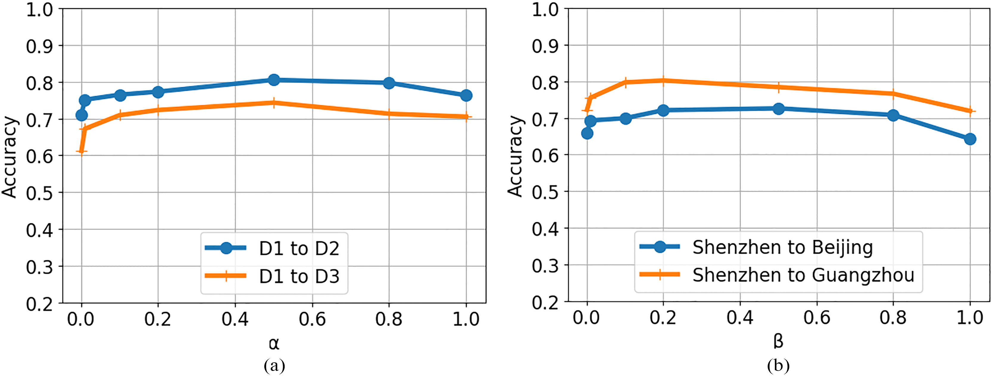
a: Sensibility with regard to $\alpha$ ; b: Sensibility with regard to $\beta$ .

The performance of MVT-DAE over another baseline can be strengthened via image classification task. According to the Table 3, the proposed approach still outperforms the others methods. The first and most interesting observations we can come up from the Table 3 is deep learning based method (Fine tuning, CAR, MVT-DAE) outperform standard transfer learning approach (IMT, DISMUTE). Such an approach confirms the effectiveness of using deep learning for knowledge transfer as it can effectively leverage the between domains discrepancy. However deep learning based approach can only reduce but cannot wholly remove the distribution shift between domains. Taking CAR as an example, the prediction accuracy drops from 67.3% to 63.5% when transfer from D1 to D2 and D1 to D3, because the categories in D2 are more closed to D1 compared to those in D3. We can see the same phenomena when performing knowledge transfer via fine tuning (from 68.3% to 64.3%). MVT-DAE is more powerful when dealing with domain discrepancy, from D1 to D2 we have 78.5% of accuracy, and from D1 to D3 we have 77.3% of accuracy. This testifies to the effectiveness of the MVT-DAE over the other baseline.

Figure 4.

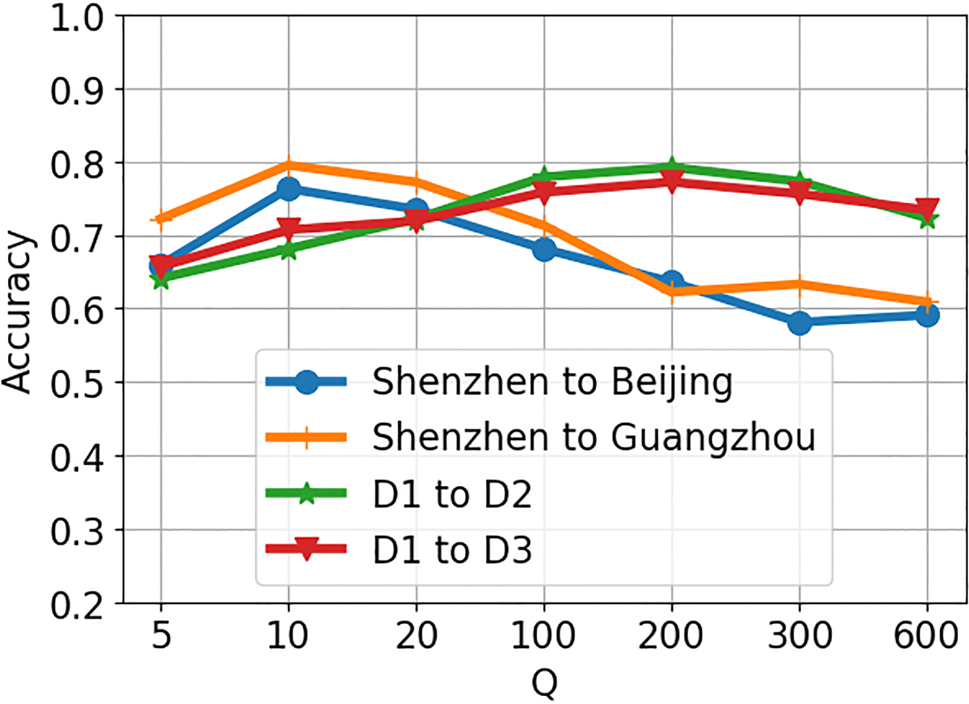
Sensibility with regard to the size of the dictionary.

Figure 5.

Accuracy over the number of iterations.

4.4.2 Parameters sensibility

The proposed approach involves two hyper-parameters $\alpha$ and $\beta$ , $\alpha$ maximizes the values of the relative weight of the JMMD whereas $\beta$ controls the weight of the selected features. We have also studied the sensibility of those two parameters. The Fig. 3 shows the transfer accuracy of MVT-DAE by varying both $\alpha$ and $\beta$ in the range {0.001 0.01 0.1 0.2 0.5 0.8 1 2}. We perform transfer task on Corel dataset from D1 to D2 and D1 to D3. From the Fig. 3 we can see the bell-shaped curve. This, confirms the effectiveness of using multi-view dictionary learning and deep auto auto-encoder empowered with JMMD to perform transfer learning in a multi-view setting.

4.4.3 The sensibility of the learned dictionaries

We have also investigated the sensibility of learned dictionaries in the source domain. We perform four transfer learning tasks namely D1 to D2, D1 to D3, Shenzhen to Beijing and Shenzhen to Guangzhou and by varying the common dimensionality of the dictionaries Q in the range {5 10 20 50 100 200 300 600}. The result of the experiment is shown in the Fig. 4. for image classifications tasks we got the best accuracy with Q $=$ 200 whereas for air quality prediction the best accuracy is given by Q $=$ 10.

4.4.4 Convergence propriety

Due to the complexity of the proposed approach, it becomes essential to verify its convergence property. We evaluate the converge on the air quality prediction data from Shenzhen to Guangzhou for the next one hour. The Fig. 5 shows the evolution of the prediction error of the target city over the number of iterations. Compared with FLORAL, the proposal approach converges faster with a more significant improvement of the accuracy during the whole procedure of the convergence.

Table 4
% and count of randomly selected observation

% of randomly

selected data

Number of

observation

From

AlexNet

From

ResNet

From

VGG16

Stripe

max pooling

Filters

max pooling

\times

\times

120

\times

160

\times

200

\times

240

\times

280

\times

320

100

120

\times

360

120

\times

Figure 6.

Accuracy over the percentage of missing values.

4.4.5 Dealing with missing observations

We study the behavior of MVT-DAE when facing missing observations in some views. To do that we randomly pick some instances from all views in the target domain and suppress them from the training data. We perform transfer task from D1 to D2 under the new setting. We vary the percentage of the missing data through the range {10%, 20%, 30%, 40%, 50%, 60%, 70%, 80% ,90%}. When applying max -pooling, we set the stripe to 1 and depending on the level of sparsity we use different filter matrix. The Table 4 shows the number of randomly selected of observation for each percentage in each view and their corresponding filter size; we report the accuracies in our experiment in the Fig. 6. According to the Fig. 6 the proposed approach is very robust to missing data. The curve stays almost steady until 60%. This shows that Max-pooling operation can effectively combat the missing instance without causing severe damage during prediction.

5. Conclusion

In this paper, we propose a novel transfer learning approach to conduct knowledge transfer from a multi-view source domain to an unlabeled and insufficient multi-view target domain. Our approach performs knowledge transfer in two stages, at the first stage we learn a new enriched representation of all views at the source domain via dictionary learning and transfer the dictionaries to the target domain. Those dictionaries will then be used to learn an enriched presentation of the target domain. We have also incorporated a max-pooling operation to combat missing values at the target domain. At the second stage, knowledge transfer is conducted via a deep auto-encoder. Two DAE are jointly trained via Joint maximum mean discrepancy; each DAE incorporates an embedding layer to reconstruct the input and a label layer to encodes the label information from the source domain. Also, we ensure only the weight of the embedding and label layer are transferred to the target domain. Extensive experiments were conducted on two different real-world datasets testifying the effectiveness of the proposed approach over multiple baselines.

References

Gretton

Borgwardt

K.M.

Rasch

M.J.

Schölkopf

and Smola

, A kernel two-sample test, Journal of Machine Learning Research (JMLR) 13 (2012), 723–773.

Krizhevsky

Sutskever

and Geoffrey

, Hinton, Imagenet classification with deep convolutional neural networks, in: Advances in Neural Information Processing Systems (NIPS), 2012.

Zhang

Liu

and Cao

, in: Low-Rank Tensor Constrained Multiview Subspace Clustering, In ICCV, 2015.

Tzeng

Hoffman

Darrell

Zhang

and Saenko

, Simultaneous deep transfer across domains and tasks, in: IEEE International Conference on Computer Vision (ICCV), 2015.

Zhong

Fan

Yang

Verscheure

and Ren

, Cross validation framework to choose amongst models and datasets for transfer learning, In: Joint European Conference on Machine Learning and Knowledge Discovery in Databases (ECML-PKDD), Springer, 2010, pp. 547–562.

Zhuang

F.Z.

Luo

Xiong

Y.H.

and Shi

Z.Z.

, Cross-domain learning from multiple sources: A consensus regularization perspective, IEEE TKDE, 2010.

Zhuang

F.Z.

Luo

Xiong

Y.H.

and Shi

Z.Z.

, in: Supervised Representation Learning: Transfer Learning with Deep Autoencoders, in: Proceedings of the Twenty-Fourth International Joint Conference on Artificial Intelligence (IJCAI 2015).

Zhuang

Cheng

Pan

and Shi

, in: Multiple source transfer learning via consensus regularization, ECML PKDD 2014, Part III, LNCS 8726, 2014, pp. 417–431.

Liu

Lin

Yan

Sun

and Ma

, Robust recovery of subspace structures by low-rank representation, in: IEEE Transactions on Pattern Analysis and Machine Intelligence 35(1) (2013), 171–184.

10.

Yosinski

Clune

Bengio

and Lipson

, How transferable are features in deep neural networks? in: Advances in Neural Information Processing Systems (NIPS), 2014.

11.

Simonyan

and Zisserman

, Very deep convolutional networks for large-scale image recognition, arXiv preprint arXiv: 1409.1556, 2014.

12.

Zhang

Ren

and Sun

, Deep residual learning for image recognition, in: IEEE Conference on Computer Vision and Pattern Recognition (CVPR), 2016.

13.

Song

Huang

Smola

Fukumizu

, Hilbert space embeddings of conditional distributions with applications to dynamical systems, in: International Conference on Machine Learning (ICML), 2009.

14.

Long

Zhu

Wang

and Jordan

M.I.

, Deep Transfer Learning with Joint Adaptation Networks, in: Proceedings of the 34th International Conference on Machine Learning, Sydney, Australia, PMLR 70, 2017.

15.

Long

Zhu

Wang

and Jordan

M.I.

, Unsupervised domain adaptation with residual transfer networks, in: Advances in Neural Information Processing Systems (NIPS), 2016, pp. 136–144.

16.

Chen

M.M.

Z.X.

Weinberger

and Sha

, Marginalized denoising autoencoders for domain adaptation, in: Proceedings of the 29th ICML (2012).

17.

Chattopadhyay

J.P.

Panchanathan

Fan

and Davidson

, Multi-source domain adaptation and its application to early detection of fatigue, in: Proceedings of the 17th ACM SIGKDD, ACM 2011, pp. 717–725.

18.

Pan

S.J.

and Yang

, A survey on transfer learning. Knowledge and Data Engineering, IEEE Transactions on 22(10) (2010), 1345–1359.

19.

Mon

and Caronell

, Completely Heterogeneous Transfer Learning with Attention-What And What Not To Transfer, in: Proceedings of twenty-Sixth International Joint Conference on Artificial Intelligence (IJCAI-17).

20.

Ganin

and Lempitsky

, Unsupervised domain adaptation by back propagation, in: International Conference onMachine Learning (ICML), 2015.

21.

Wei

Zheng

and Yang

, Transfer Knowledge between Cities, KDD ’16, August 13–17, 2016, San Francisco, CA, USA.

22.

Ding

Shao

and Fu

, Latent low-rank transfer subspace learning for missing modality recognition, in: Proceedings of the 28th AAAI Conference on Artificial Intelligence, 2014.

23.

Ding

and Fu

, Low-rank common subspace for multi-view learning, in: IEEE International Conference on Data Mining, 2014, pp. 110–119.

24.

Ding

Shao

and Fu

, Missing modality transfer learning via latent low-rank constraint, IEEE Transactions on Image Processing 24(11) (Nov 2015), 4322–4334.

25.

Ding

Shao

and Fu

, Incomplete multisource transfer learning, IEEE Transactions On Neural Networks And Learning Systems, 2016.

26.

Ding

Shao

and Fu

, Transfer learning for image classification with incomplete multiple sources, in: International Joint Conference on Neural Networks, 2016.

27.

Fang

and Zhang

Z.M.

, Discriminative feature selection for multi-view cross-domain learning, in CIKM, 2013, pp. 1321–1330.

Multi-view deep unsupervised transfer leaning via joint auto-encoder coupled with dictionary learning

Abstract

Keywords

1. Introduction

2. Related work

2.1 Transfer learning from multi-source

2.2 Transfer learning via deep auto-encoder

3. Proposed approach

3.1 Problem definition

3.2 Join Maximum mean discrepancy

3.3 MVT-DAE overview

3.4.2 Update D v

3.4.3 Update T m

3.5 Parameters transfer via deep auto-encoder

4. Empirical experiment

4.1 Dataset

4.1.1 Urban dataset

1 https://www.microsoft.com/en-us/research/people/yuzheng/#datasets.

2 http://archive.ics.uci.edu/ml/datasets/Corel+Image+Features.

4.4 Results

4.4.1 Prediction accuracy

Table 2 Classification accuracy of urban dataset for AQI prediction

4.4.3 The sensibility of the learned dictionaries

4.4.4 Convergence propriety

Table 4 % and count of randomly selected observation

5. Conclusion

References

3.4.2 Update $D_{v}$

3.4.3 Update $T_{m}$

¹
https://www.microsoft.com/en-us/research/people/yuzheng/#datasets.

²
http://archive.ics.uci.edu/ml/datasets/Corel+Image+Features.

Table 2
Classification accuracy of urban dataset for AQI prediction

Table 4
% and count of randomly selected observation